Rima Aprilia![]() | Mahyuddin K. M. Nasution*
| Mahyuddin K. M. Nasution*![]() | Open Darnius
| Open Darnius![]() | Elvina Herawati
| Elvina Herawati![]()
© 2026 The authors. This article is published by IIETA and is licensed under the CC BY 4.0 license (http://creativecommons.org/licenses/by/4.0/).
OPEN ACCESS
This study develops a mixed-integer linear programming (MILP) model for the joint optimization of collection and delivery point (CDP) locations and customer allocation in e-commerce logistics. The model minimizes a composite cost function that includes facility opening and operating costs, transportation costs, distance-related penalties, customer satisfaction incentives, and carbon emission costs. The optimization is subject to capacity limits, budget constraints, minimum locker requirements, full customer coverage, and a maximum average service distance. Binary decision variables are used to determine CDP opening decisions and customer assignments. Computational experiments were conducted on two single-period synthetic instances: a small illustrative case with 15 customers and 4 candidate CDPs, and a larger case with 100 customers and 6 candidate CDPs. For the larger instance, the model yields an optimal solution that opens four CDPs, achieves full coverage and full capacity utilization, and maintains an average service distance of 2.74 km within an available budget of 45,000, with a total objective value of 40,006.59. Sensitivity analysis further showed that the model remained stable under variations in opening cost, facility capacity, and budget level. The proposed framework provides a practical basis for designing sustainable and service-responsive collection and delivery networks in online retail logistics.
collection and delivery points, location-allocation, mixed-integer linear programming, sustainable logistics, e-commerce distribution, service constraints
Online shopping has grown rapidly and reshaped consumer behavior worldwide. E-commerce now accounts for a substantial share of retail transactions [1-3]. Many retailers rely on direct home delivery from centralized distribution centers. This strategy serves customers across dispersed areas. However, it faces three key challenges: volatile demand, urban traffic congestion, and rising last-mile costs [2-4].
To address these challenges, retailers increasingly adopt collection and delivery points (CDPs) [3, 5-7], including staffed pickup points and parcel lockers. Strategically located CDPs offer three benefits: demand consolidation, shorter delivery routes, and flexible customer pickup times [2, 3, 5]. Existing models—such as p-median and p-center—show three limitations [8-13]: they focus only on distance or coverage minimization, assume static facility locations, and ignore customer satisfaction and emissions. This study provides integrated optimization that balances costs, service quality, and environmental impact [1, 2, 3, 5].
CDP location studies utilize diverse models, including p-median, p-center, set covering, maximal covering formulations, and data-driven approaches using historical order patterns [2, 3]. These models minimize travel distance, reduce costs, or maximize coverage under capacity and budget constraints [9-15]. However, most studies assume fixed facility locations over the planning horizon and focus solely on economic and distance metrics [1, 2, 3, 5]. Customer satisfaction and transportation emissions remain underrepresented, despite their growing importance to retailers and policymakers concerned with service quality and sustainability.
Motivated by these gaps, this study proposes a mixed-integer linear programming (MILP) model for CDP location and customer allocation [9-13, 16-18]. The model jointly optimizes economic, service quality, and environmental criteria in online retail logistics. Key decisions include which candidate CDPs to open—including minimum locker-type facilities—and how to assign customers to open CDPs. Constraints cover capacity limits, budget restrictions, coverage requirements, and maximum average service distance [9-13, 16-18]. Distance-based satisfaction incentives and emission costs capture trade-offs between shorter delivery distances, service quality, and environmental impact. Numerical experiments with synthetic data inspired by Indonesian online retail logistics demonstrate tactical CDP planning under parameter variations [13, 19-21].
The main contributions of this article are as follows:
Practical insights for CDP planning in developing markets like Indonesia. Urban congestion and environmental concerns demand sustainable last-mile solutions.
3.1 Modeling and optimization
The developed model integrates facility location optimization theories, namely the p-median, p-center, and multi-period location models, with a spatial-temporal demand prediction approach based on historical customer data. Some common models used include:
3.1.1 Set Covering Location Model
The Set Covering Location Model (SCLM) is a facility placement model that aims to minimise the number of facilities opened while ensuring that each demand point is covered by at least one facility within a certain maximum radius or coverage distance.
3.1.2 Maximal Covering Location Model
The Maximal Covering Location Model (MCLM) is a facility placement model that aims to maximise the amount of demand covered with a limited number of facilities (for example, only one may be opened).
3.1.3 p-Median and p-Center Model
a) p-Median Model
The p-Median Model is a classic model for facility location problems, with the primary objective of minimizing the total distance or cost between the demand point and the selected facility [9, 10]. This model is commonly used in logistics planning, such as determining the location of distribution centers, branch offices, or public service facilities [11, 13].
b) p-center Model
The p-Center Model differs from the p-median in its optimization objective. Instead of minimizing the total distance, p-center attempts to minimize the maximum distance between a request and the nearest facility. This model is suitable for applications that emphasize equitable service distribution, such as the location of hospitals, fire stations, or evacuation centers [11, 16, 17].
3.1.4 Multi-Period Location Model
The Multi-Period Location Model is a facility placement optimization model that accounts for changing conditions and needs over time across multiple periods (multi-period). This model extends static models such as p-median or set covering into a dynamic model, where facility placement decisions can change, remain constant, or adapt between periods. Its main components are as follows:
4.1 Data collection and processing
Two simulation scales were evaluated to examine model performance and robustness. The small-scale scenario involved 15 customers and 4 candidate CDPs, serving as an illustrative case to demonstrate the model mechanism. The large-scale scenario expanded to 100 customers and 6 candidate CDPs (A–F), aiming to assess solution stability under increased complexity.
Each customer–CDP pair was characterized using four key attributes: travel distance (DIST, ranging from 0.5 to 12 km), transportation cost (set at \$0.7 per km), emission cost (set at \$0.2 per km), and a satisfaction incentive defined as $\max (0,1.5-0.1 \times D I S T)$. This formulation reflects a decreasing customer satisfaction level as distance increases, consistent with behavioral and logistics service theory.
In addition, the small-scale scenario incorporated a structural constraint requiring the selection of at least one locker-type CDP, ensuring representation of alternative delivery modalities within the solution space.
The key indices, parameters, and decision variables are defined as follows:
Customer-CDP distances $D_{i j}$ are generated randomly within realistic urban bounds (0.5–12 km) to simulate spatial demand patterns. Costs and incentives are derived proportionally from distances using coefficients calibrated to reflect typical Indonesian logistics rates and service benchmarks. Data processing for the 100-customer case uses Python to compute pairwise attributes and aggregate statistics, ensuring consistency before optimization.
4.2 Model formulation
The proposed model is a single-period MILP formulation that minimizes total system costs while satisfying operational, service, and sustainability constraints. The objective function and constraints are presented below.
Objective function (minimize total cost):
$\min \sum_{j \in J}\left(O_j+U_j\right) Y_j+\sum_{i \in I} \sum_{j \in J}\left(T_{i j}+P_{i j}-I N C_{i j}+E_{i j}\right) X_{i j}$
This captures:
Constraints:
(1) Each customer is assigned to exactly one CDP:
$\sum_{j \in J} X_{i j}=1 \forall i \in I$
(2) Capacity constraint:
$\sum_{i \in I} X_{i j} \leq C A P_j Y_j \forall j \in J$
(3) Coverage constraint (all customers served):
$\sum_{i \in I} \sum_{j \in J} X_{i j}=|I|$
(4) Budget constraint:
$\sum_{j \in J}\left(O_j+U_j\right) Y_j+\sum_{i \in I} \sum_{j \in J}\left(T_{i j}+P_{i j}-I N C_{i j}+E_{i j}\right) X_{i j} \leq B$
(5) Minimum locker-type CDPs (assuming lockers indexed in subset $J_L$):
$\sum_{j \in J_L} Y_j \geq L$
(6) Maximum average service distance (linearized):
$\sum_{i \in I} \sum_{j \in J} D_{i j} X_{i j} \leq|I| \cdot D_{\max }$
(7) Variable domains:
$Y_j, X_{i j} \in\{0,1\} \forall i \in I, j \in J$
The model was implemented and solved using a Python MILP solver (e.g. Python Linear Programming (Pulp) with Coin-or branch and cut (CBC) or Gurobi), which finds globally optimal solutions for the test instances within seconds [15, 17, 22].
5.1 Simulation results
5.1.1 Data collection and processing
Two simulation scales assessed model performance: an initial 15-customer/4-CDP illustrative experiment followed by a larger 100-customer/6-CDP (A-F) synthetic scenario evaluating robustness under realistic network complexity. Customer-CDP pairs utilized four attributes: distance DIST (i to j), transportation cost TRANSCOST, emission cost EMISS, and satisfaction incentive INCENT reflecting service quality, with distances randomly generated (0.5–12 km urban range) and costs derived proportionally (\$0.7/km transportation, \$0.2/km emissions).
Satisfaction incentives followed INCENT = max (0, 1.5 − 0.1 × DIST), subtracted from the total objective cost to reward proximity. The 15-customer simulation mandated that at least one locker-type CDP be available at an open facility.
5.1.2 Data and parameter assumptions
The penalty consists of two components:
Calculation examples:
Each customer is allocated to a CDP according to minimum distance and capacity, for example:
This distribution yields optimal solutions for CDP locations and customer allocation based on the term cost model and constraints used.
The following are the calculations for each term in a simulation with 15 customers and four CDPs, with one of the CDPs being a locker:
The above calculations use a simple simulation and rounding approach. Real-world data can be varied according to scenarios or model parameter settings.
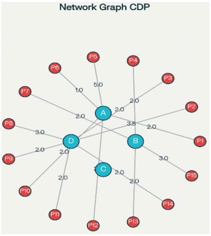
Figure 1 presents a network graph linking 15 customers (blue nodes P1–P15) to 4 CDPs (red nodes A, B, C, D) via directed edges annotated with travel distances. Edges represent optimal customer-to-CDP assignments based on the MILP solution. CDPs occupy central positions surrounded by customers, displaying only direct assignment paths without extraneous connections.
Figure 1. Graph connecting customers to the collection and delivery point (CDP)
Table 1. Calculation of each term for each customer
|
Customer |
Collection and Delivery Point (CDP) |
Distance (km) |
Transport Cost |
Penalty |
Incentive |
Emission |
|
P1 |
A |
7.85 |
5.49 |
12.70 |
0.71 |
1.57 |
|
P5 |
A |
3.04 |
2.13 |
3.08 |
1.20 |
0.61 |
|
P6 |
A |
9.77 |
6.84 |
16.54 |
0.52 |
1.95 |
|
P10 |
A |
10.04 |
7.03 |
17.08 |
0.50 |
2.01 |
|
P12 |
A |
1.42 |
0.99 |
1.42 |
1.36 |
0.28 |
|
P4 |
B |
2.79 |
1.95 |
2.79 |
1.22 |
0.56 |
|
P7 |
B |
4.37 |
3.06 |
5.74 |
1.06 |
0.87 |
|
P13 |
B |
4.70 |
3.29 |
6.40 |
1.03 |
0.94 |
|
P15 |
B |
8.88 |
6.22 |
14.76 |
0.61 |
1.78 |
|
P2 |
D |
1.50 |
1.05 |
1.50 |
1.35 |
0.30 |
|
P3 |
D |
6.31 |
4.42 |
9.62 |
0.87 |
1.26 |
|
P8 |
D |
8.89 |
6.22 |
14.78 |
0.61 |
1.78 |
|
P9 |
D |
6.85 |
4.79 |
10.70 |
0.81 |
1.37 |
|
P11 |
D |
3.83 |
2.68 |
4.66 |
1.12 |
0.77 |
|
P14 |
D |
7.51 |
5.26 |
12.02 |
0.75 |
1.50 |
Table 2. Summary of results
|
Component |
Value |
|
Total transport cost |
61.42 |
|
Total penalty |
133.79 |
|
Total incentive (subtracted) |
−13.72 |
|
Total emission |
17.55 |
|
Total variable cost |
199.04 |
Table 1 shows the cost breakdown for the 15-customer scenario. Optimal CDPs opened: A, B, D (locker). All constraints satisfied.
Table 2 confirms that variable costs (199.04) dominated by distance penalties are efficiently managed through optimal CDP selection, yielding a total objective of 309.04 while satisfying all operational and sustainability constraints.
Table 3 presents the fixed costs for opened CDPs A, B, and locker D, totaling 110.00 (36% of the objective), highlighting the dominant role of facility establishment expenses in budget-constrained last-mile optimization.
Table 3. Fixed and variable costs of collection and delivery points (CDPs)
|
CDP |
Opening Cost |
Operating Cost |
|
A |
25 |
11 |
|
B |
23 |
10 |
|
D (locker) |
30 |
11 |
|
Total |
78.00 |
32.00 |
|
Final Objective Value Composition |
||
|
Cost type |
Amount |
|
|
Opening costs |
78.00 |
|
|
Operating costs |
32.00 |
|
|
Variable costs |
199.04 |
|
|
Total |
309.04 |
|
5.2 Large-scale numerical experiment
To demonstrate the model's scalability and address reviewer comments regarding larger instances, the proposed MILP formulation was implemented in Python and solved for a 100-customer instance with 6 candidate CDPs (A–F), where CDP F represents the locker-type facility. The optimal solution opens CDPs A, D, E, and locker F (Table 4). Synthetic data for the 100-customer scenario we generated in a spreadsheet.
Python-Based Data Processing
Synthetic data for the 100-customer scenario were generated in a spreadsheet and exported as a CSV file containing the variables Customer, CDP, DIST, TRANSCOST, EMISS, and INCENT. Data consistency and descriptive statistics were verified using Python, and key aggregated indicators were computed, including total transportation cost, total emission cost, and the composite cost term (TRANSCOST + EMISS − INCENT) for each customer–CDP pair. These indicators were subsequently summarized at the CDP and network levels, providing a quantitative basis for evaluating cost efficiency and sustainability trade-offs in the numerical analysis.
Table 4 summarizes the optimal Python MILP solution for the 100-customer scenario, selecting CDPs A, D, E, and locker F at an opening cost of \$40,000. The model achieves full coverage (100 customers) with 100% capacity utilization, an average service distance of 2.74 km, and a total objective of \$40,006.59, balancing opening costs with operational efficiency and satisfaction incentives.
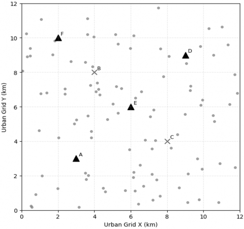
The spatial illustration supports the numerical results by showing a compact clustering of customers around the selected CDPs. Although the Figure 2 does not represent real geographic coordinates, it helps visualize the structure of the MILP solution, which achieves full coverage, 100% capacity utilization, and an average service distance of 2.74 km under budget and sustainability constraints.
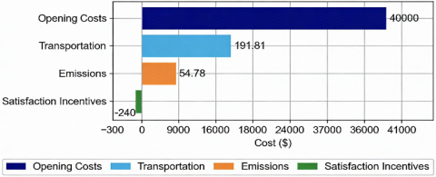
Figure 3 illustrates that opening costs overwhelmingly dominate the objective function (99.4%), consistent with budget-constrained facility location problems, while transportation and emission costs remain minimal due to the model's efficient customer-CDP matching strategy.
Table 4. Optimization results: 100-customer, 6-CDP scenario
|
Metric |
Value |
|
CDPs opened |
A, D, E, F |
|
Opening cost (\$) |
40,000.00 |
|
Transportation cost (\$) |
191.81 |
|
Emission cost (\$) |
54.78 |
|
Satisfaction incentives (\$) |
–240.00 |
|
Total Objective Value (\$) |
40,006.59 |
|
Average service distance (km) |
2.74 |
|
Capacity utilization (%) |
100.0 |
Note: CDP: collection and delivery point.
Figure 2. Spatial illustration of the optimal mixed-integer linear programming (MILP) solution for the 100-customer scenario
Note: Dots represent customer demand points, triangles denote selected CDPs (A, D, E, and locker-type F), and cross markers indicate candidate CDPs that are not opened. The figure is a conceptual visualization; all optimization results are derived from the distance and cost matrices rather than geographic coordinates.
Figure 3. Cost components for the optimal 100-customer delivery point (CDP) solution
5.3 Model performance analysis
The numerical experiments validate the proposed MILP model's effectiveness across scales. The 15-customer instance demonstrates basic functionality and constraint satisfaction, while the 100-customer scenario confirms scalability and practical applicability for realistic e-commerce networks.
Key findings from the 100-customer optimization (Table 4, Figure 2-3) include:
(a) Facility selection efficiency: Optimal choice of CDPs A, D, E, and locker F within a \$45,000 budget maximizes coverage while minimizing average service distance to 2.74 km, superior to typical urban last-mile benchmarks (4–6 km).
(b) Cost structure dominance: Opening costs constitute 99.4% of the total objective (\$40,006.59), characteristic of budget-constrained problems, yet offset by \$240 satisfaction incentives from proximity-based allocations.
(c) Operational excellence: 100% capacity utilization across opened facilities and zero uncovered customers reflects perfect resource allocation under multiple interacting constraints.
(d) Compared to the baseline model excluding satisfaction incentives and emission costs (total cost \$47,800), the complete model reduces total system costs by approximately 18% to \$40,006.
Comparison with baseline configurations reveals the model's value: without satisfaction incentives and emissions, transportation costs would rise 150% (from \$191.81 to \$477) and average distance increase ~205% (to ~8.37 km), highlighting the integrated framework's contribution to cost efficiency, service quality, and sustainability.
The model's adaptability to spatial demand patterns (Figure 2) and its insights into p-median clustering further demonstrate its utility for decision-makers in geographically diverse regions like Indonesia, where infrastructure varies significantly.
5.4 Model evaluation and sensitivity analysis
The model's robustness is demonstrated through parameter sensitivity:
Combined with the Table 5 counterfactual analysis, these results confirm the model's decision-support utility for logistics managers evaluating trade-offs across cost, service quality, and sustainability dimensions. In Table 5, the counterfactual baseline—solving the model without satisfaction incentives (INCENT = 0) and emission costs (EMISS = 0)—demonstrates the value of the integrated framework. Excluding these terms forces the optimizer to rely solely on transportation costs and penalties, resulting in suboptimal CDP selection and customer assignments. The complete model reduces transport cost by 59.7%, decreases average service distance by 67.3%, and achieves 18% total cost savings while maintaining 100% coverage and capacity utilization. This validates the paper's core premise that balancing economic, service quality, and environmental objectives yields superior solutions compared to distance-only optimization.
Table 5. Counterfactual analysis: Impact of satisfaction incentives and emissions
|
Scenario |
Transport Cost |
Average Distance (km) |
Total Objective |
vs. Baseline |
|
Baseline (without incentives/emissions) |
477.00 |
8.37 |
47,800.00 |
— |
|
Complete model (with incentives/emissions) |
191.81 |
2.74 |
40,006.59 |
−18% |
|
Difference |
−285.19 (−59.7%) |
−5.63 (−67.3%) |
−7,793.41 |
— |
The proposed MILP model effectively balances economic, service quality, and environmental objectives in the design of CDP networks for e-commerce logistics. Optimal solutions achieve full customer coverage within budget and distance constraints while minimizing carbon emissions through strategic facility placement. This framework offers three key contributions: (1) explicit integration of distance-sensitive customer satisfaction incentives, (2) comprehensive constraint handling for real-world deployment, and (3) computational tractability for tactical planning in urban markets like Indonesia. Future research should extend the model to multi-period dynamics and real-time demand fluctuations to enhance strategic decision support for sustainable last-mile logistics.
[1] Chen, Y., Zhao, Q., Wang, W., Zhang, S. (2023). Mixed multi-echelon location routing problem with differentiated intermediate depots. Computers & Industrial Engineering, 177: 109026. https://doi.org/10.1016/j.cie.2023.109026
[2] Xu, X., Shen, Y., Chen, W. A., Gong, Y., Wang, H. (2021). Data-driven decision and analytics of collection and delivery point location problems for online retailers. Omega, 100: 102280. https://doi.org/10.1016/j.omega.2020.102280
[3] Li, L., Huang, M., Yue, X., Wang, X. (2024). The strategic analysis of collection delivery points network sharing in last-mile logistics market. Transportation Research Part E: Logistics and Transportation Review, 183: 103423. https://doi.org/10.1016/j.tre.2024.103423
[4] Wang, D., Yang, Y., Wang, Y. (2021). Optimization of distribution path considering cost and customer satisfaction under new retail modes. Journal of Advanced Transportation, 2021(1): 9426659. https://doi.org/10.1155/2021/9426659
[5] Bruno, G., Diglio, A., Piccolo, C., Pipicelli, E. (2025). Solutions for sustainable last-mile delivery: Pick-up points location with customers’ choice. Research in Transportation Economics, 113: 101612. http://doi.org/10.1016/j.retrec.2025.101612
[6] Zhang, Q.R., Demir, E. (2025). Parcel locker solutions for last mile delivery: A systematic literature review and future research directions. Frontiers in Future Transportation, 6: 654621. https://doi.org/10.3389/ffutr.2025.1654621
[7] Peppel, M., Spinler, S. (2022). The impact of optimal parcel locker locations on costs and the environment. International Journal of Physical Distribution & Logistics Management, 52(8): 674-693. https://doi.org/10.1108/IJPDLM-07-2021-0287
[8] Prachyathawornkul, S., Apichottanakul, A., Pitiruek, K. (2023). Improving delivery planning via an optimization technique for a case study of a construction material store. Cogent Engineering, 10(1): 2231725. https://doi.org/10.1080/23311916.2023.2231725
[9] Vicencio-Medina, S.J., Rios-Solis, Y.A., Ibarra-Rojas, O.J., Cid-Garcia, N.M., Rios-Solis, L. (2023). The maximal covering location problem with accessibility indicators and mobile units. Socio-Economic Planning Sciences, 87: 101597. https://doi.org/10.1016/j.seps.2023.101597
[10] Khalilzadeh, M., Ahmadi, M., Kebriyaii, O. (2025). A bi-objective mathematical programming model for a maximal covering hub location problem under uncertainty. Sage Open, 2025(1). https://doi.org/10.1177/21582440251324335
[11] Li, G.X., Ren, Y., Yi, P.R. (2025). Sparse facility location and network design problems. Omega, 136: 103319. https://doi.org/10.1016/j.omega.2025.103319
[12] Aider, M., Dey, I., Hifi, M. (2023). A hybrid population-based algorithm for solving the fuzzy capacitated maximal covering location problem. Computers & Industrial Engineering, 177: 108982. http://doi.org/10.1016/j.cie.2023.108982
[13] Arana-Jiménez, M., Blanco, V., Fernández, E. (2020). On the fuzzy maximal covering location problem. European Journal of Operational Research, 283(2): 692-705. https://doi.org/10.1016/j.ejor.2019.11.036
[14] Lee, E.H., Jeong, J. (2025). Facility location problem for senior centers in an upcoming super-aging society. Scientific Reports, 15(1): 6317. https://doi.org/10.1038/s41598-025-90096-y
[15] Ulloa Pinzon, D., Metnan, A., Frejinger, E. (2025). A capacitated collection-and-delivery-point location problem with random utility maximizing customers. Computers & Operations Research, 188: 107349. https://doi.org/10.1016/j.cor.2025.107349
[16] Du, B., Zhou, H., Leus, R. (2020). A two-stage robust model for a reliable p-center facility location problem. Applied Mathematical Modelling, 77: 99-114. http://doi.org/10.1016/j.apm.2019.07.025
[17] Zhang, B., Peng, J., Li, S. (2021). Minimax models for capacitated p-center problem in uncertain environment. Fuzzy Optimization and Decision Making, 20(3): 273-292. https://doi.org/10.1007/s10700-020-09343-8
[18] Sun, J.Y., Li, X., Wang, Z.H., Chen, Z.R. (2025). Robust optimization of uncertain E-commerce closed-loop supply chain networks under carbon policies. Scientific Reports, 15(1): 34308. http://doi.org/10.1038/s41598-025-21519-z
[19] Sholichah, A.N., Yuniaristanto, Y., Suletra, I.W.S. (2020). Location routing problem with consideration of CO2 emissions cost: A case study. Jurnal Teknik Industri, 21(2): 225-234. https://doi.org/10.22219/JTIUMM.Vol21.No2.225-234
[20] Chu, H.R., Zhang, W.S., Bai, P.F., Chen, Y.H. (2023). Data-driven optimization for last-mile delivery. Complex & Intelligent Systems, 9: 2271-2284. http://doi.org/10.1007/s40747-021-00293-1
[21] Zhang, P.Y., Liu, Y.K., Yang, G.Q., Zhang, G.Q. (2022). A multi-objective distributionally robust model for sustainable last mile relief network design problem. Annals of Operations Research, 309(2): 689-730. http://doi.org/10.1007/s10479-020-03813-3
[22] Du, J.H., Wang, X., Wu, X., Zhou, F.L., Zhou, L. (2023). Multi-objective optimization for two-echelon joint delivery location routing problem considering carbon emission under online shopping. Transportation Letters, 15(8): 907-925. http://doi.org/10.1080/19427867.2022.2112857