Nadjet Chettih*![]() | Ahlam Labdaoui
| Ahlam Labdaoui![]() | Dounia Keddari
| Dounia Keddari![]() | Farah Boutouatou
| Farah Boutouatou![]()
© 2026 The authors. This article is published by IIETA and is licensed under the CC BY 4.0 license (http://creativecommons.org/licenses/by/4.0/).
OPEN ACCESS
Accurate classification of inflow regimes supports reservoir operation and risk-informed water management, yet it remains challenging due to nonlinear hydroclimatic dynamics and temporal dependence. This study proposes an advanced hybrid mathematical modeling framework that integrates long short-term memory (LSTM) networks with extreme gradient boosting (XGBoost) to improve the classification accuracy of inflow regimes in complex dam systems. The LSTM component was employed to capture deep temporal dependencies from a 17-year hydrometeorological dataset of the Beni Haroun Dam, sourced from the National Agency for Dams and Transfers (ANBT) in Algeria, while the XGBoost classifier provides robust nonlinear decision boundaries for final classification. The proposed hybrid model is consistently evaluated against five benchmark machine learning (ML) classifiers, along with the standalone LSTM and XGBoost models: gradient boosting (GB), logistic regression (LR), support vector machine (SVM), k-nearest neighbors (KNN), and Gaussian naïve bayes (GNB). The results indicate that the hybrid LSTM–XGBoost framework reaches a predictive performance level of 99.12% accuracy, 99.15% precision, 99.09% recall, 99.12% F1-score, 99.50% specificity, 0.99 Cohen’s Kappa, and 0.88% Mean Classification Error (MCE). These findings demonstrate that the hybrid deep ensemble strategy presented here provides a robust mathematical and computational framework for intelligent dam management, environmental risk assessment, and sustainable hydrological planning at the Beni Haroun Dam under increasing climatic variability.
classification, deep learning, hydrological resource management, reservoir operation, long short-term memory, XGBoost, Algeria
Water resource management is essential to the sustainable development of the world, and is especially important in areas where climate change significantly affects dam operations and water supply. The precise forecasting of water inflow to dams is vital for effective operation, flood risk reduction, and ensuring a reliable water supply for domestic, agricultural, and industrial uses. However, modeling inflow dynamics remains challenging because hydrometeorological parameters are highly nonlinear and interdependent. In this context, inflow classification plays a critical role in modern hydrological management systems, enabling dam operators to anticipate different inflow conditions, such as low, medium, or high flows, thereby supporting strategic planning for water release, storage, and flood control. Precise inflow classification also improves drought preparedness, supports equitable water distribution among sectors, and ensures downstream ecosystem stability. Consequently, constructing reliable inflow classification models is essential for smart and sustainable reservoir operations under increasing climatic uncertainty.
Artificial intelligence (AI) has emerged as a powerful tool for capturing complex nonlinear interactions among hydrometeorological variables [1]. Numerous studies have highlighted the predictive capabilities of machine learning (ML) and deep learning (DL) approaches for evaporation and inflow forecasting. Tezel and Buyukyildiz [2] demonstrated that artificial neural networks (ANNs) and support vector machines (SVMs) can accurately forecast monthly pan evaporation, outperforming traditional methods. Similarly, Deo et al. [3] applied a relevance vector machine (RVM), extreme learning machine (ELM), and multivariate adaptive regression splines (MARS) to predict evaporation, showing that ML can identify the most relevant predictors and improve accuracy. Wu et al. [4] developed hybrid ELM-based models that incorporate whale optimization algorithm (WOA) and flower pollination algorithm (FPA) for monthly evaporation forecasting in the Poyang Lake Basin, achieving higher success rates than traditional techniques. Shabani et al. [5] used random forest (RF), Gaussian process regression (GPR), and k-nearest neighbors (KNN) to predict evaporation, confirming ML’s strength in capturing nonlinear relationships among climatic parameters. Despite these advances, challenges remain in selecting reliable ML models for hydrological forecasting, particularly regarding model interpretability, computational efficiency, and sensitivity to data quality [6, 7].
The considerable size and complexity of hydrometeorological data further complicate the analysis and modeling. These datasets often consist of variables measured at different time points, requiring efficient techniques to identify patterns and relationships that enhance hydrological understanding and improve forecasting accuracy. ML effectively handles nonlinear relationships among climatic and hydrological variables, whereas DL excels at handling unstructured or complex data. The choice between ML and DL depends on the data structure, model complexity, and available computational resources. To leverage the strengths of both, hybrid models that integrate ML and DL are gaining attention for their improved adaptability, accuracy, and robustness in hydrological forecasting.
This study applies a hybrid deep ensemble learning framework to the Beni Haroun Dam, combining LSTM’s temporal feature extraction with XGBoost's robust classification performance to enhance inflow classification performance. The main contributions of this work are as follows: (1) the development of a hybrid LSTM–XGBoost model that exploits the complementary strengths of ML and DL, (2) a systematic evaluation of the hybrid model against standalone ML and DL approaches to quantify performance improvements, and (3) the application of the framework to a 17-year hydrometeorological dataset of the Beni Haroun Dam, offering insights for intelligent dam management and sustainable water resource planning in the region. The outcomes demonstrate the potential of data-driven models to support decision-making in reservoir operations under climatic variability in the Beni Haroun Dam.
The remainder of this paper is structured as follows: Section 2 presents the materials and methods used in this study. Section 3 provides the background knowledge relevant to the proposed approach. Section 4 describes the modeling framework and implementation details. Section 5 presents and discusses the experimental results. Finally, Section 6 concludes the paper by summarizing the main findings of the study and outlining directions for future work.
2.1 Study area
The data used in this research were obtained from the daily hydrometeorological records at the Beni Haroun Dam station (Figure 1), provided by the National Agency for Dams and Transfers (ANBT), which covers the period from 1st September 2003 to 31st December 2020. For the duration of the study, several climatic and hydrological parameters were continuously monitored to gain a better understanding of the dam's operation dynamics and environmental conditions.
The input and target variables used in this study are defined as follows:
The target variable, inflow class, represents the total incoming water volume during a given period and is categorized into three inflow levels (low, medium, and high), integrating the combined effects of climatic inputs, catchment runoff, and upstream transfers.
These variables constitute the input features for the ML models developed to predict reservoir inflow dynamics and support water resources management.
Figure 1. Location of the Beni Haroun Dam, Algeria
2.2 Experimental setup
All experiments were conducted on a workstation with the following configuration: Microsoft Windows 11 Professional 64-bit (Build 22000), powered by an Intel® Core™ i9-10900K processor (10 cores, 20 threads, 3.70 GHz base frequency), and equipped with 32 GB of installed physical memory (RAM). The system includes an NVIDIA GeForce RTX 3060 Ti GPU with 8 GB of dedicated VRAM. All experiments were executed using Python 3.11.7 within an Anaconda-managed environment on this hardware platform.
2.3 Methodology overview
A hybrid classification framework (Figure 2) combining DL and ML was developed to predict inflow classes for the Beni Haroun Dam. The approach integrates LSTM networks for deep feature extraction with extreme gradient boosting (XGBoost) for classification, organized into three stages: (i) preparation and preprocessing of the hydrometeorological dataset, (ii) deep feature extraction using the LSTM network followed by classification with XGBoost, alongside a set of comparative ML models, and (iii) model evaluation based on different performance metric.
2.3.1 Data preparation and standardization
Hydrometeorological data from the Beni Haroun Dam were preprocessed without missing values. Features were standardized using z-score normalization to ensure uniform scaling and enhance model convergence. The dataset was split into 60% training, 20% validation, and 20% testing subsets to enable unbiased evaluation.
2.3.2 Deep feature extraction and XGBoost classification
An LSTM network was employed to extract latent temporal features, leveraging its capacity to model nonlinear and sequential dependencies. The extracted embeddings were input to an XGBoost classifier, selected for its efficiency, regularization capabilities, and ability to handle complex nonlinear patterns. Hyperparameters for both LSTM and XGBoost were optimized to maximize classification performance, resulting in a robust hybrid framework with improved accuracy and generalization.
2.3.3 Comparative models
For benchmarking, classical ML models, including gradient boosting (GB), logistic regression (LR), support vector machine (SVM), KNN, and Gaussian naive bayes (GNB), were trained under identical conditions.
2.3.4 Model evaluation
Performance was assessed using multiple metrics: Accuracy, Precision, Recall, F1-score, Specificity, Misclassification Error, and Cohen’s Kappa coefficient.
(a) Step 1: Dataset
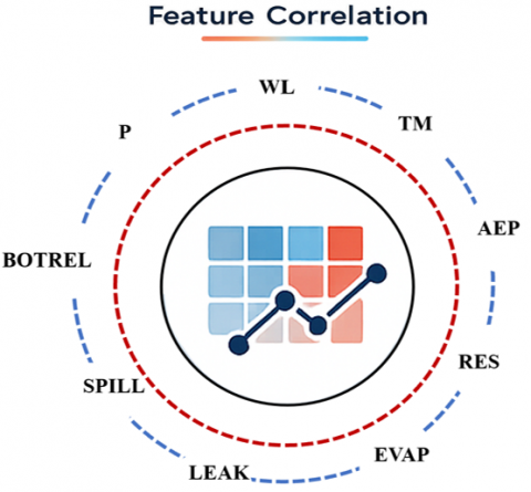
(b) Step 2: Features correlation
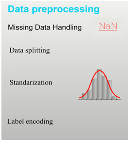
(c) Step 3: Data preprocessing
(d) Step 4: Modelling
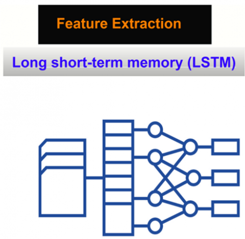
(e) Step 5: Feature extraction
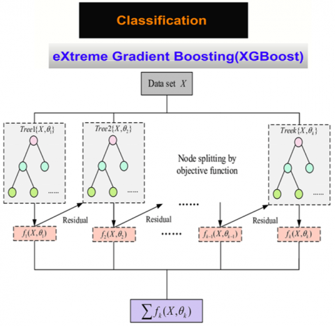
(f) Step 6: Classification
(g) Step 7: Performance evaluation

(h) Step 8: Comparison
Figure 2. Methodology pipeline of the proposed work
This section defines the basic concepts needed to elaborate on our classification methods and presents the theoretical foundations of the models used, with particular emphasis on the formal mathematical formulations of the LSTM network and the XGBoost algorithm. Their rigorous representation clarifies underlying mechanisms and supports the methodological developments that follow.
3.1 Long short-term memory
Recurrent Neural Networks (RNNs) are commonly used to model sequential dependencies by linking inputs across time steps. However, standard RNNs often face challenges in capturing long-term dependencies due to vanishing or exploding gradients. To address these limitations, the LSTM network illustrated in Figure 3 was developed as an improved RNN variant, capable of effectively retaining and leveraging past information over extended sequences.
An LSTM unit comprises three primary gating mechanisms, input gate $\left(i_t\right)$, forget gate $\left(f_t\right)$, and output gate $\left(o_t\right)$, which collectively regulate the flow of information within the network. The input gate determines the extent of new information to be incorporated into the memory cell ($c_t$), while the forget gate decides which parts of the previous memory should be discarded. The interaction between these two gates results in an updated cell state that encapsulates both new and retained information. The output gate controls the degree to which the internal memory is exposed to the next layer or time step, thus generating the final output $\left(h_t\right)$ of the LSTM unit.

Figure 3. Long short-term memory (LSTM) architecture
Mathematically, the behavior of an LSTM cell can be described as follows:
$\begin{aligned} f_t & =\phi\left(W_f y_{t-1}+b_f\right) \\ i_t & =\phi\left(W_i y_{t-1}+b_i\right) \\ o_t & =\phi\left(W_o y_{t-1}+b_o\right) \\ \tilde{c}_t & =\psi\left(W_c y_{t-1}+b_c\right) \\ c_t & =f_t \otimes c_{t-1} \oplus i_t \otimes \tilde{c}_t \\ h_t & =o_t \otimes \psi\left(c_t\right)\end{aligned}$
Here, $\phi$ and $\psi$ represent the sigmoid and hyperbolic tangent activation functions, respectively; ⊗ and ⊕ denote element-wise multiplication and addition; and $W$ and $b$ correspond to the weight matrices and bias vectors associated with the respective gates. Figure 3 illustrates the fundamental architecture of the LSTM model.
The incorporation of this memory mechanism enables LSTM networks to preserve contextual information over long sequences, making them highly effective for tasks involving temporal or sequential data.
3.2 Extreme gradient boosting
XGBoost is a decision tree-based boosting ensemble algorithm that offers greater efficiency, scalability, and flexibility than traditional GB Decision Trees [8]. Being a distributive GB framework, it is known for fast computation and high predictive performance. XGBoost follows the basic concept, whereby an ensemble of weak learners, mostly decision trees, is constructed sequentially. Each newly grown tree is taught to target the residual errors of the previous trees to fine-tune the overall accuracy [9, 10]. It employs a sparsity-aware algorithm and a weighted quantile sketch for approximate tree learning, whereby large-scale datasets with billions of examples can be efficiently handled [8].
Additionally, XGBoost optimizes an arbitrary differentiable loss function, allowing it to capture complex data patterns more effectively than conventional methods [11]. Its popularity in ML competitions can be attributed to its robust predictive performance, compatibility with distributed processing frameworks, and advanced system-level features such as cache-aware access patterns, data compression, and sharding [8].
In the context of a classification task, consider an ensemble composed of $K$ additive classification trees. The prediction for the $i$-th instance $x_i$ is defined as:
$\hat{y}_i=\sum_{k=1}^K f_k\left(x_i\right)$ (1)
where, $f_k$ denotes the function learned by the $k$-th decision tree. The overall objective function is a combination of the loss function and a regularization term:
${Obj}(\theta)=\sum_{i=1}^n l\left(y_i, \hat{y}_i\right)+\sum_{k=1}^K \omega\left(f_k\right)$ (2)
Here, $l$ is a differentiable convex loss function measuring the discrepancy between the true label $y_1$ and prediction $\hat{y}_1$, and $\omega\left(f_k\right)$ is a regularization function penalizing the complexity of the $k$-th tree. At the $t$-th boosting round, the prediction is updated as:
$\hat{y}_i^{(t)}=\hat{y}_i^{(t-1)}+f_t\left(x_i\right)$ (3)
The objective at this step is:
${Obj}^{(t)}=\sum_{i=1}^n l\left(y_i, \hat{y}_i^{(t-1)}+f_t\left(x_i\right)\right)+\omega\left(f_t\right)$ (4)
To facilitate optimization, the loss function is approximated using a second order Taylor expansion:
$x_{1,2}=\frac{-b \pm \sqrt{b^2-4 a c}}{2 a}$ (5)
${Obj}^{(t)} \approx \sum_{i=1}^n\left[g_i f_t\left(x_i\right)+\frac{1}{2} h_i f_t^2\left(x_i\right)\right]+\omega\left(f_t\right)+const$ (6)
where the first and second-order gradients, respectively.
$g_i=\frac{\partial}{\partial \hat{y}_i^{(t-1)}} l\left(y_i, \hat{y}_i^{(t-1)}\right)$ (7)
$h_i=\frac{\partial^2}{\partial \hat{y}_i^{(t-1)^2}} l\left(y_i, \hat{y}_i^{(t-1)}\right)$ (8)
Neglecting constant terms, the simplified objective becomes:
${Obj}^{(t)} \approx \sum_{i=1}^n\left[g_i f_t\left(x_i\right)+\frac{1}{2} h_i f_t^2\left(x_i\right)\right]+\omega\left(f_t\right)$ (9)
The regularization term is defined as:
$\omega(f)=\gamma T+\frac{1}{2} \lambda \sum_{j-1}^T w_j^2$ (10)
where, $T$ is the number of leaves, $w_j$ is the weight of the $j$-th leaf, $\gamma$ controls tree complexity, and $\lambda$ is the L2 regularization parameter. Let $I_j=\left\{i \mid q\left(x_i\right)=j\right\}$ be the set of instances in leaf $j$. The objective can then be rewritten as:
${Obj}^{(\mathrm{t})} \approx \sum_{j=1}^T\left[\left(\sum_{i \in I_j} g_i\right) w_j+\frac{1}{2}\left(\sum_{i \in I_j} h_i+\lambda\right) w_j^2\right]+\gamma T$ (11)
Let $G_j=\sum_{i \in I_j} g_i$ and $H_j=\sum_{i \in I_j} h_i$, then:
$O b j^{(t)}=\sum_{j-1}^T\left[G_j w_j+\frac{1}{2}\left(H_j+\lambda\right) w_j^2\right]+\gamma T$ (12)
This formulation allows for efficient learning through greedy expansion, leveraging both first and second-order gradient information.
4.1 Data preprocessing
4.1.1 Imputation of missing data
Missing data in environmental monitoring datasets can compromise the reliability of water quality modeling [12, 13]. Various imputation strategies have been proposed, with median-based methods often proving robust against skewed distributions and outliers [14, 15]. In this study, no missing values were present; therefore, all observations were retained in their original form to preserve the dataset’s integrity and ensure accurate classification of hydrological inflow patterns.
4.1.2 Outliers treatment
In hydrological modeling, maintaining the natural distribution of environmental indicators is essential for preserving data authenticity. Rather than removing statistical outliers, this study adopts a data retention strategy, acknowledging that extreme values often reflect meaningful hydrological variations rather than noise [16-18]. All observed values of inflow-related parameters were retained without transformation. This approach ensures that rare but ecologically significant events are captured, allowing the models to learn from the full variability of the Beni Haroun Dam system and remain robust under changing hydroclimatic conditions.
4.1.3 Label encoding
The target variable in this study comprised three categorical inflow classes, each representing distinct hydrological states of the Beni Haroun Dam. To ensure compatibility with ML algorithms, the class labels were transformed into numerical values using label encoding [19, 20]. Formally, for the set of class labels.
L = {l₀, l₁, l2}
where, l₀, l1 and l2 correspond to the set of class labels. The label encoding function LE is formally defined as:
$\mathrm{LE}\left(\mathrm{l}_{\mathrm{i}}\right)=\mathrm{i}, \forall \mathrm{l}_{\mathrm{i}} \in \mathrm{L}, \mathrm{i} \in\{0,1,2\}$
This approach preserves class identity while providing an efficient numerical representation for models.
4.1.4 Data splitting
To ensure a robust evaluation of the model’s generalization capability, a stratified split was employed, allocating 60% of the samples for model training, 20% for validation during training, and the remaining 20% for independent testing. This proportion provides an optimal balance between learning, hyperparameter tuning, and evaluation, allowing the model to effectively capture the underlying data distribution while preserving representative validation and test sets for unbiased performance assessment.
4.1.5 Feature scaling
In this study, feature scaling was performed to normalize the range of input variables, ensuring that all features contributed equally to the learning process. This preprocessing step prevents variables with larger magnitudes from disproportionately influencing model training [21, 22]. The StandardScaler technique was employed to standardize each feature Xj, for j=1,…,n, to have zero mean and unit variance, as defined by the transformation:
$X_{\text {scaled}, \,j}=\frac{X_j-\mu_j}{\sigma_j}$
where, μj is the mean of feature Xj, and σj is its standard deviation.
4.1.6 Features correlation
The correlation matrix presented in Figure 4 illustrates the linear correlation among the hydrological and meteorological variables of the Beni Haroun Dam over a 17-year observation period. Linear associations were quantified using Pearson's correlation, where values close to +1 indicate strong positive correlation, values close to –1 indicate strong negative correlation, and values near 0 indicate weak or negligible linear association. The results showed several important linear correlations. A strong positive correlation (r = 0.73) exists between EVAP and TM, suggesting that higher air temperatures are directly associated with increased evaporation from the dam surface. WL exhibits moderate positive correlations (r = 0.40) with both AEP and LEAK, indicating that higher dam levels tend to correspond with greater water transfers and seepage rates. A weak positive correlation (r = 0.37) between P and RES reflects that rainfall contributes moderately to dam storage. Conversely, BOTREL shows negative correlations with WL (r = –0.34) and EVAP (r = –0.23), implying that bottom releases tend to occur when dam levels and evaporation rates are lower. Importantly, the generally low to moderate correlation values among most features indicate that the variables are not highly redundant and that each provides unique and complementary information about the system’s behavior. Overall, the correlation analysis highlights the interdependence of dam dynamics while confirming that the diversity of weakly correlated features enriches the dataset. This strengthens the predictive modeling of inflow classes, as it allows the algorithms to learn from multiple independent sources of variability, improving the overall robustness and generalization of the model for reservoir management and water resource forecasting.

Figure 4. Correlation matrix heatmap of the study variables
4.2 Model evaluation
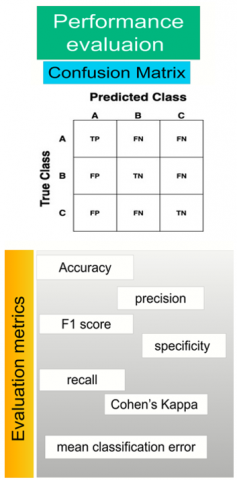
4.2.1 The confusion matrix
The confusion matrix is a fundamental tool in ML for evaluating classification model performance [23]. It displays actual versus predicted classes in a tabular format, where rows represent true labels and columns represent predicted labels [24].
For each class, the confusion matrix provides four key outcomes:
Although originally developed for binary classification, the confusion matrix extends naturally to multiclass problems, where performance is analyzed per class and then averaged [25]. From this matrix, several metrics are derived: accuracy, precision, recall, F1-score, specificity, Mean Classification Error (MCE), and Cohen’s Kappa to provide a comprehensive evaluation.
A single measure may not capture all aspects of model behavior. This study adopts a multi-metric evaluation approach to ensure robust and reliable assessment across all inflow categories. The detailed structure and relationships among predicted and actual inflow classes are illustrated in Figure 5.
The overview below presents a summary of classification performance metrics discussed in Table 1.

Figure 5. Confusion matrix for multi-class classification
Table 1. Overview of classification performance metrics
|
Metric |
Definition |
Formula |
|
Accuracy |
Signifies the proportion of instances correctly predicted out of the total instances in the dataset. |
Accuracy $=\frac{T P+T N}{T P+T N+F P+F N}$ |
|
Precision |
Also called positive predictive value; calculates the proportion of true positives among all instances predicted as positive. |
Precision $=\frac{T P}{T P+F P}$ |
|
Recall |
Measures the model’s ability to correctly identify positive instances in the dataset. |
Recall $=\frac{T P}{T P+F N}$ |
|
F1-Score |
A composite metric combining precision and recall into a single value. |
F1-Score $=2 \times \frac{\text { Precision × Recall }}{\text { Precision }+ \text { Recall }}$ |
|
Specificity |
Also called the true negative rate, measures the proportion of actual negatives correctly identified. |
Specificity $=\frac{T N}{T N+F P}$ |
|
Mean Classification Error (MCE) |
The average error across all classes. |
MCE $=1-\frac{T P+T N}{{ Total\ number\ of \ samples }}$ |
|
Kappa Statistic |
Measures inter-rater agreement or reliability, accounting for chance agreement. |
$\kappa=\frac{p_o-p_e}{1-p_e}$ where, p₀ represents the observed agreement and pₑ the expected agreement by chance. |
5.1 Performance of single LSTM and XGBoost models
The hyperparameters for both the LSTM and XGBoost models were selected using a trial-and-error approach. For the LSTM, the number of units, dropout rate, batch size, and learning rate were adjusted to achieve stable convergence and prevent overfitting, using the validation set to guide tuning. For XGBoost, parameters including the number of estimators, learning rate, maximum tree depth, subsample ratio, and regularization terms (reg_alpha, reg_lambda) were tuned iteratively using features extracted from the LSTM on the training set, with validation data employed for early stopping and hyperparameter selection. The final model performance was then evaluated on the independent test set. This strategy ensured a robust hybrid model with optimized predictive accuracy while maintaining manageable computational costs.
LSTM architecture was configured with two stacked LSTM layers comprising 128 and 64 memory cells, respectively, each followed by a 0.3 dropout regularization rate. A fully connected dense layer with 32 neurons and ReLU activation was applied before the final softmax output layer, which generated class probabilities for the three target categories. The network was optimized using the Adam optimizer with a fixed learning rate of 0.001 and trained with a categorical cross-entropy loss function.
The training process employed mini-batches of 32 samples for 100 epochs, with early stopping applied to halt training upon convergence of the validation loss. Weight initialization followed the Glorot Uniform scheme, and L2 regularization λ of 0.001 was imposed on the dense layer to ensure generalization and stability.
Table 2 summarizes the performance of LSTM, XGBoost, and the proposed hybrid model.
The LSTM network achieved an accuracy of 97.20%, demonstrating its ability to capture the complex temporal dependencies and sequential relationships inherent in the dataset. The high precision (97.13%) and recall (97.38%) indicate that the model effectively identified true positives while minimizing false positives, reflecting both high sensitivity and robust generalization. The F1-score of 97.24% and specificity of 98.50% further confirmed a balanced performance in distinguishing positive and negative samples. From a statistical perspective, Cohen’s Kappa of 0.96 and an MCE of 2.80% indicate strong agreement between the predicted and true labels with minimal misclassification.
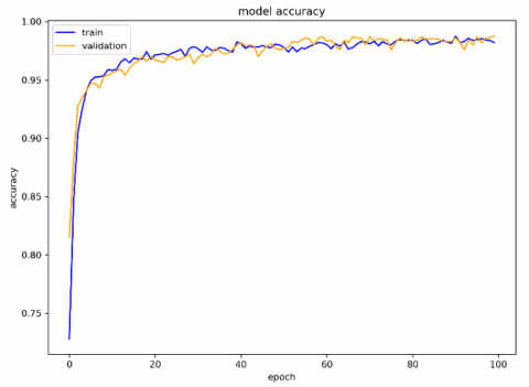
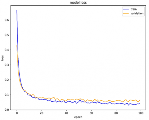
The training and validation curves presented in Figures 6 and 7 illustrate the convergence behavior of the proposed LSTM network during model optimization, showing the evolution of model accuracy across 100 epochs for both training and validation sets. The two curves rapidly increase within the first 10 epochs, stabilizing around a high accuracy level thereafter. There are several indications of model generalization to unseen data, given the absence of divergence between training and validation accuracies. The training process was smooth, and no noticeable divergence between the training and validation curves was observed, which is an indicator that overfitting was not present, and the network successfully captured the underlying temporal dependencies without memorizing the training data.
These plots confirm that the LSTM achieved stable learning and excellent convergence behavior, maintaining a balance between bias and variance. This stability validates the LSTM’s suitability as a feature extraction mechanism, enabling it to learn compact, discriminative temporal representations of the inflow-related variables. In subsequent stages, these deep LSTM features are leveraged by the XGBoost classifier, which capitalizes on their informative structure to achieve enhanced classification performance. The absence of overfitting in the LSTM phase ensures that the extracted features remain generalizable, thereby improving the reliability and interpretability of the hybrid LSTM–XGBoost framework.
Table 2. Performance comparison of LSTM, XGBoost, and the proposed hybrid model across training and testing phases
|
Classifier |
Phase |
Accuracy (%) |
Precision (%) |
F1-Score (%) |
Recall (%) |
Specificity (%) |
Mean Classification Error (%) |
Kappa |
|
LSTM |
Train |
98.52 |
98.24 |
98.53 |
98.85 |
99.29 |
1.48 |
0.98 |
|
Test |
97.20 |
97.13 |
97.24 |
97.38 |
98.50 |
2.80 |
0.96 |
|
|
XGBoost |
Train |
95.37 |
95.59 |
95.34 |
95.10 |
97.36 |
4.63 |
0.93 |
|
Test |
93.75 |
93.95 |
93.70 |
93.47 |
96.44 |
6.25 |
0.90 |
|
|
Proposed model |
Train |
99.80 |
99.83 |
99.80 |
99.77 |
99.88 |
0.20 |
1.00 |
|
Test |
99.12 |
99.15 |
99.12 |
99.09 |
99.50 |
0.88 |
0.99 |
Note: LSTM = long short-term memory; XGBoost = networks with extreme gradient boosting
Figure 6. Training and validation accuracy curves of the LSTM model during the learning phase
Figure 7. Training and validation loss curves of the LSTM model during the learning phase
An XGBoost classifier was employed to model complex nonlinear relationships within the dataset by aggregating a large number of weak learners into a powerful ensemble. The classifier was configured with 500 estimators and a maximum tree depth of six, balancing model expressiveness and generalization capability. A learning rate of 0.05 was adopted to ensure gradual convergence and prevent overfitting. To enhance diversity among trees, subsample and column-sample-by-tree ratios were both set to 0.8, allowing partial feature and sample usage per iteration. Regularization terms (α = 0.001, λ = 1.0) were applied to control model complexity and reduce variance, while Gamma (0.1) imposed a minimum loss threshold for split creation. The XGBoost classifier achieved an overall accuracy of 93.75%, capturing the complex nonlinear relationships in the structured tabular data. The precision (93.95%) and recall (93.47%) reflect its ability to balance false positives and true positives, whereas an F1-score of 93.70% and specificity of 96.44% indicate strong performance across all classes. Cohen’s Kappa of 0.90 and MCE of 6.25% confirm the model’s stability and generalization capability.
5.2 Interpretation of hybrid LSTM-XGBoost model performance
The hybrid LSTM–XGBoost model achieved a high accuracy of 99.12%, representing the most advanced and comprehensive predictive framework among the single LSTM and XGBoost models.
This hybrid integration capitalizes on the complementary strengths of both paradigms. LSTM’s ability to autonomously extract high-level temporal and contextual embeddings, and XGBoost’s powerful ensemble-based discrimination capability optimized for structured tabular data. In the proposed hybrid framework, the LSTM network first performs deep feature extraction, transforming the raw input into a compact, information-rich latent representation. These deep features are then passed to the XGBoost classifier, which operates as a meta-learner capable of refining decision boundaries based on the extracted representations. This architecture effectively combines DL’s representational expressiveness with XGBoost’s gradient-based interpretability, producing a combination enhancement in model performance. As summarized in Table 2, the hybrid model achieved a precision of 99.15%, a recall of 99.09%, and an F1-score of 99.12%, confirming its ability to accurately classify both positive and negative in the hybrid model stances with minimal misclassification. The specificity of 99.50% further underscores the model’s outstanding capability to correctly identify negative samples, ensuring highly reliable discrimination across all classes. The Cohen’s Kappa coefficient of 0.99 signifies near-perfect agreement between the predicted and actual labels, reflecting exceptional consistency and reliability beyond random chance. Additionally, the MCE of just 0.88% demonstrates almost negligible misclassification, emphasizing the hybrid model’s robustness and stability. This level of performance surpasses the individual LSTM and XGBoost models and highlights the latent potential of hybrid deep ensemble architectures in high-stakes data modeling tasks.

Figure 8. LSTM confusion matrix

Figure 9. Networks with extreme gradient boosting (XGBoost) confusion matrix

Figure 10. The proposed model confusion matrix
The results substantiate that deep sequential learning can significantly enrich the feature space of GB algorithms, enhance class separability, and mitigate residual classification errors. Such findings challenge the prevailing assumption that ensemble boosting methods are inherently self-sufficient in feature extraction. Instead, the hybrid results demonstrate that even sophisticated tree-based learners can substantially benefit from deep, non-linear embeddings generated by neural architectures like LSTM.
The confusion matrices displayed in Figures 8-10 illustrate the comparative performance of the three models. Figure 10 corresponds to the proposed hybrid model, while Figures 8 and 9 represent the standalone LSTM and XGBoost models, respectively. The confusion matrix shows that the LSTM model achieves strong results, with 295, 310, and 607 correct predictions for Classes 0, 1, and 2, respectively. However, several Class 2 samples are misclassified as Class 1, indicating difficulty in distinguishing closely related inflow categories. Similarly, XGBoost produce 283, 293, and 594 correct classifications, but shows greater confusion between Classes 0, 1, and 2 due to its lack of temporal feature learning. In contrast, the hybrid model achieves the highest classification accuracy, with 300, 314, and 623 correctly predicted instances and minimal misclassifications across all classes.
These visualizations suggest that the hybrid architecture effectively captures both the sequential dynamics and nonlinear relationships inherent in hydrological inflow data.
5.3 Comparison with machine learning models
The proposed hybrid model was benchmarked against conventional algorithms, including GB, LR, SVM, KNN, and GNB. As shown in Table 3, it consistently outperformed all alternatives in terms of the evaluation metrics, with respective accuracy of 95.43%, 94.55%, 88.42%, 86.06%, and 58.09%.
These results highlight the hybrid model’s capacity to capture complex nonlinear interactions missed by traditional approaches, delivering highly reliable and high-precision predictions suitable for advanced water resource management.
Table 3. Performance comparison of the proposed hybrid model and baseline classifiers during training and testing phases
|
Model |
Phase |
Accuracy (%) |
Precision (%) |
Recall (%) |
F1 (%) |
Specificity (%) |
Mean Classification Error (%) |
Kappa |
|
Gradient boosting |
Train |
97.96 |
98.34 |
97.58 |
97.95 |
98.74 |
2.04 |
0.97 |
|
Test |
95.43 |
95.46 |
95.41 |
95.43 |
97.45 |
4.57 |
0.92 |
|
|
Logistic regression |
Train |
95.03 |
95.26 |
94.82 |
95.03 |
97.17 |
4.97 |
0.92 |
|
Test |
94.55 |
94.55 |
94.60 |
94.57 |
96.99 |
5.45 |
0.91 |
|
|
Support vector machine |
Train |
89.32 |
90.38 |
88.07 |
89.08 |
93.65 |
10.68 |
0.83 |
|
Test |
88.62 |
89.35 |
87.66 |
88.42 |
93.36 |
11.38 |
0.82 |
|
|
K-nearest neighbors |
Train |
90.71 |
91.19 |
90.09 |
90.61 |
94.65 |
9.29 |
0.85 |
|
Test |
86.06 |
86.82 |
85.10 |
85.88 |
91.93 |
13.94 |
0.77 |
|
|
Gaussian naive bayes |
Train |
58.97 |
70.66 |
70.42 |
61.66 |
81.10 |
41.03 |
0.42 |
|
Test |
58.09 |
69.36 |
69.98 |
60.24 |
80.79 |
41.91 |
0.41 |
|
|
Proposed model |
Train |
99.80 |
99.83 |
99.80 |
99.77 |
99.88 |
0.20 |
1.00 |
|
Test |
99.12 |
99.15 |
99.12 |
99.09 |
99.50 |
0.88 |
0.99 |
This study shows that combining LSTM-based feature extraction with XGBoost improves inflow prediction performance at the Beni Haroun Dam. The proposed hybrid framework consistently outperforms standalone LSTM and other ML models across multiple evaluation metrics, confirming its robustness and reliability. By integrating the deep representational capacity of LSTM with the predictive efficiency of XGBoost, the model effectively captures complex nonlinear and uncertain hydrological patterns while maintaining computational efficiency.
Despite these advantages, several limitations should be acknowledged. The hybrid model relies on a fixed set of input variables and may underperform if key hydrological or meteorological features are missing or unavailable. Its predictive accuracy could also decrease when extreme events or rare inflow patterns are not adequately represented in the training data. In addition, the model captures temporal dependencies at a single scale, without explicitly accounting for multi-scale or seasonal dynamics. Finally, computational demands increase with dataset size, which may limit real-time deployment for large-scale reservoir networks.
To address these limitations and further enhance the proposed framework, future research should focus on incorporating multimodal data sources, including hydrological observations, meteorological parameters, and remote sensing imagery. The fusion of these complementary information streams would enable a more comprehensive representation of the physical processes governing inflow variability. Such an integrative approach is expected to improve the model’s generalization capability, enhance predictive performance, and ultimately support more reliable and data-driven reservoir management strategies.
|
$\alpha$ |
learning rate |
|
$\gamma$ |
regularization parameter |
|
$\lambda$ |
L2 regularization term |
[1] Chen, L., Han, B., Wang, X.S., Zhao, J.Z., Yang, W., Yang, Z. (2023). Machine learning methods in weather and climate applications: A survey. Applied Sciences, 13(21): 12019. https://doi.org/10.3390/app132112019
[2] Tezel, G., Buyukyildiz, M. (2016). Monthly evaporation forecasting using artificial neural networks and support vector machines. Theoretical and Applied Climatology, 124: 69-80. https://doi.org/10.1007/s00704-015-1392-3
[3] Deo, R.C., Samui, P., Kim, D. (2016). Estimation of monthly evaporative loss using relevance vector machine, extreme learning machine and multivariate adaptive regression spline models. Stochastic Environmental Research and Risk Assessment, 30: 1769-1784. https://doi.org/10.1007/s00477-015-1153-y
[4] Wu, L., Huang, G., Fan, J., Ma, X., Zhou, H., Zeng, W. (2020). Hybrid extreme learning machine with meta-heuristic algorithms for monthly pan evaporation prediction. Computers and Electronics in Agriculture, 168: 105115. https://doi.org/10.1016/j.compag.2019.105115
[5] Shabani, S., Samadianfard, S., Sattari, M.T., Mosavi, A., Shamshirband, S., Kmet, T., Várkonyi-Kóczy, A.R. (2020). Modeling pan evaporation using Gaussian process regression, K-nearest neighbors, random forest and support vector machines: Comparative analysis. Atmosphere, 11(1): 66. https://doi.org/10.3390/atmos11010066
[6] Ahmadi, S.M., Balahang, S., Abolfathi, S. (2024). Predicting the hydraulic response of critical transport infrastructures during extreme flood events. Engineering Applications of Artificial Intelligence, 133: 108573. https://doi.org/10.1016/j.engappai.2024.108573
[7] Ghiasi, B., Noori, R., Sheikhian, H., Zeynolabedin, A., Sun, Y., Jun, C., Hamouda, M., Bateni, S.M., Abolfathi, S. (2022). Uncertainty quantification of granular computing-neural network model for prediction of pollutant longitudinal dispersion coefficient in aquatic streams. Scientific Reports, 12(1): 4610. https://doi.org/10.1038/s41598-022-08417-4
[8] Chen, T., Guestrin, C. (2016). XGBoost: A scalable tree boosting system. In KDD '16: Proceedings of the 22nd ACM SIGKDD International Conference on Knowledge Discovery and Data Mining, San Francisco, California, USA, pp. 785-794. https://doi.org/10.1145/2939672.2939785
[9] Liang, W., Luo, S., Zhao, G., Wu, H. (2020). Predicting hard rock pillar stability using GBDT, XGBoost, and LightGBM algorithms. Mathematics, 8(5): 765. https://doi.org/10.3390/math8050765
[10] Zhang, W.G., Li, H.R., Wu, C.Z., Li, Y.Q., Liu, Z.Q., Liu, H.L. (2021). Soft computing approach for prediction of surface settlement induced by earth pressure balance shield tunneling. Underground Space, 6(4): 353-363. https://doi.org/10.1016/j.undsp.2019.12.003
[11] Fafalios, S., Charonkytakis, P., Tsamardinos, I. (2020). Gradient boosting trees. https://api.semanticscholar.org/CorpusID:222288735.
[12] Zhang, Y., Thorburn, P.J. (2021). Handling missing data in near real-time environmental monitoring: A system and a review of selected methods. Future Generation Computer Systems, 128: 63-72. https://doi.org/10.1016/j.future.2021.09.033
[13] Rodríguez, V.G., Sanchez-Castillo, M., Chica-Olmo, M., Chica-Rivas, M. (2021). Machine learning predictive models for mineral prospectivity: An evaluation of neural networks, random forest, regression trees and support vector machines. Ore Geology Reviews, 71: 804-818. https://doi.org/10.1016/j.oregeorev.2015.01.001
[14] Ochieng’Odhiambo, F. (2020). Comparative study of various methods of handling missing data. Mathematical Modelling and Applications, 5(2): 87-93. https://doi.org/10.11648/j.mma.20200502.14
[15] Lee, H., Yun, S. (2024). Strategies for imputing missing values and removing outliers in the dataset for machine learning-based construction cost prediction. Buildings, 14(4): 933. https://doi.org/10.3390/buildings14040933
[16] Karydis, M. (1994). Environmental quality assessment based on the analysis of extreme values: A practical approach for evaluating eutrophication. Journal of Environmental Science and Health A, 29(4): 775-791. https://doi.org/10.1080/10934529409376071
[17] Wilby, M.J., Keller, C.U., Snik, F., Korkiakoski, V., Pietrow, A.G. (2017). The coronagraphic modal wavefront sensor: A hybrid focal-plane sensor for the high-contrast imaging of circumstellar environments. Astronomy & Astrophysics, 597: A112. https://doi.org/10.1051/0004-6361/201629150
[18] Iliev, N.I., Marinov, M., Radukanov, S. (2021). Development of algorithm for treatment of extreme outliers in numerical data, conditional on joint distribution relationship. In 2021 IEEE 8th International Scientific-Practical Conference Problems of Infocommunications Science and Technology (PIC S&T 2021), Kharkiv, Ukraine, pp. 52-56. https://doi.org/10.1109/PICST54195.2021.9772204
[19] Bellur, A.P., VL, V.K., K, S.C., Kodipalli, A., Rao, T., V, P. (2023). Water quality assessment using machine learning: A comparative analysis. In 2023 International Conference on Computational Intelligence for Information, Security and Communication Applications (CIISCA), Bengaluru, India, pp. 320-325. https://doi.org/10.1109/CIISCA59740.2023.00068
[20] Ravindra, K., Kumar, S., Kumar, A., Mor, S. (2024). Enhancing accuracy of air quality sensors with machine learning to augment large-scale monitoring networks. npj Climate and Atmospheric Science, 7: 326. https://doi.org/10.1038/s41612-024-00833-9
[21] Wan, X. (2019). Influence of feature scaling on convergence of gradient iterative algorithm. Journal of Physics: Conference Series, 1213: 032021. https://doi.org/10.1088/1742-6596/1213/3/032021
[22] Protić, D., Stanković, M., Prodanović, R., Vulić, I., Stojanović, G.M., Simić, M., Ostojić, G., Stankovski, S. (2023). Numerical feature selection and hyperbolic tangent feature scaling in machine learning-based detection of anomalies in computer network behavior. Electronics, 12(19): 4158. https://doi.org/10.3390/electronics12194158
[23] Haghighi, S., Jasemi, M., Hessabi, S., Zolanvari, A. (2018). PyCM: Multiclass confusion matrix library in Python. Journal of Open Source Software, 3(25): 729. https://doi.org/10.21105/joss.00729
[24] Piegorsch, W.W., Bailer, A.J. (1997). Statistics for Environmental Biology and Toxicology. Chapman & Hall/CRC. https://www.routledge.com/Statistics-for-Environmental-Biology-and-Toxicology/Bailer-Piegorsch/p/book/9780412047312.
[25] Markoulidakis, I., Markoulidakis, G. (2024). Probabilistic confusion matrix: A novel method for machine learning algorithm generalized performance analysis. Technologies, 12(7): 113. https://doi.org/10.3390/technologies12070113