Adeleke Aderibigbe*![]() | Abel Airoboman
| Abel Airoboman![]() | Felix Agbetuyi
| Felix Agbetuyi![]() | Anthony Adoghe
| Anthony Adoghe![]()
© 2025 The authors. This article is published by IIETA and is licensed under the CC BY 4.0 license (http://creativecommons.org/licenses/by/4.0/).
OPEN ACCESS
The electrical power system can be viewed in three parts, which includes generation, transmission and distribution systems. The poor reliability of power supply to consumers with regard to the distribution level has raised many concerns about its economic impact on both utility providers and consumers. The growth in demand for electrical power due to economic activities, urbanization and per capital energy consumption has made the expansion of the existing distribution system inevitable. This expansion faces significant obstacles. Therefore, the inability of conventional power system to meet this demand has warranted the need for the integration of Distributed Renewable Generations (DRGs) at the distribution level to enhance the network reliability. This paper, therefore, presents a study on how to optimally integrate DRGs into a real distribution network to enhance reliability enhancement using an improved cuckoo search technique, thereby reducing the time taken for convergence associated with cuckoo search algorithm. The line and load parameters with reliability data of WAEC 11 kV distribution network were collected, processed and analysed. Backward-Forward Sweep method in the MATLAB 2021 software environment was used to determine the power loss and reliability indices values both with and without DGs integration. The base case results revealed a power loss of 2120 kW at Bus 85, with a minimum voltage of 0.9368 with high reliability indices values recorded. Therefore, with 3DGs injected the power loss reduced to 926.6 kW, and the voltage at Bus 85 improved to 0.95924. The percentage reduction in SAIFI, SAIDI, CAIDI and ASUI are 1.28%, 22.96%, 21.96% and 21.96% respectively, resulting in enhanced reliability.
distributed renewable generation, reliability enhancement, cuckoo search algorithm, backward-forward sweep, MATLAB
The electrical power system comprises three key parts: generation, transmission and distribution systems [1]. The failure of vertical approach system that is of transmitting power from generation through the transmission to the load centre has inherent technical losses leading to increase in interruption frequency and interruption duration of power supply resulting in poor reliability of power supply to the consumers with severe economic impact. The poor reliability of power supply to consumers particularly at the distribution level raised many concerns on economic impact on both the utility provider and consumers. One of the solutions to vertical approach system is to extend the existing power system to cater for the increase in power demand but unfortunately large-scale facilities construction faces significant obstacle [2]. It is also established that 90% of power losses and frequent interruptions can be traced to the distribution network thereby making distribution network vulnerable to frequent interruption [3]. The increase in the demand for electrical power has made the expansion of the existing distribution networks inevitable. However, this increase faces significant obstacles when building large-scale facilities (power plants and transmission networks). Therefore, researchers and utility companies are looking for feasible, time-saving and economical techniques to cope with the demand and subsequently improve poor power system reliability. The solution proposed by most researchers revolves around Distributed Renewable Generations (DRGs) [4]. Increased interest in renewable energy resources comes from the desire to have clean, cheap and reliable electric power in line with the Sustainable Development Goals (SDGs) which project affordable and Clean Energy, Sustainable Cities and Communities and Responsible Consumption and Production termed SDG 7, SDG 11 and SDG 12 respectively. These discentralized and modular distributed renewable generation can be installed quickly by utilities or end users without the need for large scale utility projects with their insistence bottlenecks. However, how to properly and carefully site, locate and integrate these decentralized and modular distributed generation in the distribution network and with what method is a source of concern. This necessitated this research work with the development of an improved cuckoo search algorithm for optimal DRGs sizing and positioning in a large and real distribution network.
This leads us to review the views of other researchers in the same field of study.
2.1 Review the impact of distributed generator (DGs) on reliability
Adoghe et al. [5] accessed the development in Nigeria power sector from 1898 till date by analysing the reforms utilized in the power sector by pasts and present government using integrative review process in conjunction with Scopus database. The result obtained shows reduction in power outages and frequent interruption frequency and interruption duration of power supply to the consumers.
Energy storage system reliability contribution to a distribution system was assessed by Gautam and Karki [6] using modified Roy Bilintin Test system (MRBTS). MRBTS was used after modelling photovoltaic (PV) and energy storage system (ESS) with the reliability indices values improved the whole system remarkably with injected energy storage. However, impact of auxiliary component degradation, detailed reliability cost, economic studies, cost benefit analysis and worth analysis on the distribution was suggested for further studies.
Aderibigbe et al. [7] carried out a review study on the optimal placement of distributed generation for reliability improvement. The results for the study affirmed that for system adequacy and reliability, optimal placement of DG remains sacroscant for effective energy delivery.
Adefarati and Bansal [8] integrated renewable energy resources and storage system in Roy Billiton test distribution for reliability impact analysis. These are implemented in Markov model for evaluating the reliability values. It was observed that the stochastic renewable energy sources cut down cost and also improved system reliability. The question here is will using bigger distribution network gives the same result.
Ahmad and Asar [9] assessed the impact of distributed generation as a source in a Roy Billinton Test System distribution system in relation to its reliability using artificial neural network (ANN) technique in sizing and placing distributed generation optimally in the distribution system. The obtained results showed a reduction in System Average Interruption Frequency Index (SAIFI), System Average Interruption Duration Index (SAIDI) and Expected Energy Not Supplied (EENS) values by 40%, 25% and 25% respectively after DG injection. However, for future work dynamic modelling should be addressed instead of static models. Escalera et al. [10] injected distributed generation and energy storage system in order to find their effects on reliability of a real distribution ESS was modelled, based on hourly load values representation with varying generation. A significant improvement in reliability was recorded with conventional and wind DG technology compared to PV. Moreover, a high reduction in SAIDI was noticed with ESS/PV and ESS/Wind distributed generation. However, do we expect the same result when load models of different types of loads are used.
Ndawula et al. [11] assessed the injection of uncertainty distributed generation reliability impact in Medium Voltage (MV) and Low Voltage (LV) distribution networks. These are modelled with the loads and thereafter implemented in Monte Carlos simulation method to determine reliability indices. The result recorded a reduction in ENS, frequency and duration of interruption when EMS was employed.
Badr and Kalantari [12] assessed the integration of distributed generation reliability effects in RBTS Bus 2 and Bus 6. These are implemented in an improved classification algorithm to evaluate and calculate system reliability values with and without micro grids. The result obtained after applying a proposed algorithm for the analysis indicate improved reliability and that customers and system topology contributed to the feet.
Mahmoud et al. [13] assessed how the injection of distributed energy resources affects the reliability of 33/11 kV RBTS Bus 2. Evaluation and calculation of reliability indices were carried out by Dig-Silent software after modelling. Different studies conducted reveal that optimal DGs location was responsible for reliability improvement. Load points reliability issues were suggested for further study.
Gana et al. [14] assessed the impact of embedded generation on reliability of 11 kV Ran feeder in Bauchi distribution network using modified particle swarm optimization (MPSO) for optimal location and sizing of DG and Electrical Transient Analyzer Program (ETAP) software for modelling and evaluating the reliability indices. The results showed that optimal sizing and placement improved and enhanced reliability. Also, as the number of DG integration increases the more reliable the network is.
Enyew et al. [15] assessed a 33 kV two feeder radial distribution system as test system using analytical enumeration and Monte Carlo Simulation with the aim of improving reliability, minimizing power loss and proper sizing and locating DG. DIgSILENT and HOMER software tools were used for optimization of DG cost. The results showed a 97.8% reduction in SAIFI and Customer Average Interruption Duration Index (CAIDI), SAIDI by 76%, Average System Availability Index (ASAI) increased by 14.38%, ASUI reduced by 76%. This resulted into power loss reduction of 0.32 MW and utility recording more profit with DG integration.
Ghosh [16] assessed the impact of distributed generation on test systems IEEE 33 and 69-Bus with the objective of evaluating and improving the reliability of mesh-grid representation of the network. Components failure rate and network configuration are also assessed. Particle swarm optimization method was used for optimal sizing and location of DGs. The mesh-grid approach was used to configure the network by demarcating cells to form series, parallel and combination of both resulting in sub-component regions. These individual mesh reliabilities are modelled differently for determining the overall reliability. The results showed a reliability values of 0.786627861 and 0.941764534 in case of 33-Bus while in the case of 69-Bus the lowest and highest availability varies between 0.8352702 and 0.9801987. Ghaedi and Mirzadeh [17] investigated the impact of tidal height variation on the reliability of barrage type tidal power plants using Roy Bilinton Test System (RBTS) as test system. The variable failure rate of each component, based on the rise in temperature were evaluated by using Arrhenios law. Also, each component was modelled thermally. Simulation was conducted using Monte Carlos simulation and analytical method to determine power system adequacy and reliability assessment of composite power system of tidal power plants. Three approaches were considered given the same results for reliability indices values for LOLE and EENS. Also, improvement in reliability indices was recorded with the addition of tidal power plants.
2.2 Review the impact of DGs on losses and voltage trend
Agbetuyi et al. [18] considered embedded generation integration effect on Nigeria power system using Ogba 33 kV as a case study. Neplan software was used to perform load flow analysis with and without gas turbine and diesel generator connection on the network. Simulation results showed that improvement in voltage profile from 0.881 p. u to 0.958 p. u with active power loss reduction of 78.16%.
The effects of optimal sizing and siting of distributed generation on distribution network was investigated by Ogunsina et al. [19] using IEEE 32-Bus as test system and Ant Colony Algorithm for sizing and siting DG on the distribution network. The obtained results indicated that with ACO based approach there were 92% and 97% reduction in real and reactive power losses respectively compared with other approaches. The paper, however, recommends planning and dispatching of renewable energy sources due to their variables for future studies.
Airoboman et al. [20] explored how the proper siting and sizing of capacitors can improve voltage stability and system efficiency, even when the grid faces N-1 contingency conditions. Their work clearly showed the value of capacitor optimization, but it did not consider the growing role of distributed generation, which can significantly influence load flow and voltage profiles. This gap suggests that future studies need to look at capacitor planning alongside distributed generation to reflect the realities of today’s power systems.
Ahmadi et al. [21] carried out voltage profile evaluation of distribution system with renewable distributed generations using 33/11 kV Roy Billiton (RBTS) as test system. This system was modelled and simulated using Monte Carlos simulation tools and at the same time cuckoo search algorithm Reddy P et al. [22] used Firefly optimization method for optimal placement and sizing of distributed generation in distribution system using IEEE 33-Bus as test distribution system. After simulation, the result showed an improved voltage profile. This method is only suitable for single objective function.
Somefun et al. [23] conducted research on how to size and position embedded generators in power system utilizing Inherent Structural Network Topology (ISNT) and Forward-Backward Methods for DG positioning and sizing respectively. The obtained result shows the efficacy of the model in terms of losses minimization and voltage profile enhancement.
Nasir et al. [24] assessed the impact of optimal placement and sizing of distributed generation in a practical 69-Bus radial distribution system using Modified Lightning Search Algorithm (MLSA). The suitable location and size in the distribution system are identified by weighted summation and MLSA approach. Also, MATLAB software was used in modelling load profile, DGs constant load and solar load in the distribution system. The result obtained showed significant reduction in power losses and improvement in voltage profiles. Ali et al. [25] investigated the impact of distributed generation in radial electrical distribution network, 33-Bus test system using hybrid algorithm SAPSO. Here, simulated annealing (SA) and particle swarm optimization (PSO) in combination with loss sensitivity index (LSI) were used to determine the optimal location and at the same time reduced the simulation period thereby reaching the optimal solution in time. This hybrid algorithm eliminates random generation and updating problem associated with SA with avoidance of local minima problem known PSO for. The result showed the system reaching optimal solution in shorter time with reduction in power losses and improvement in voltage profile. Salman et al. [26] assessed the influence of distributed generation injected on 132 kV feeder as a test system. The test system was examined and modeled in the ETAP with and without DGs aimed at improving voltage profile and system power loss. The result showed that with right DG size and ideal position, there was increase in voltage profile and reduction in power losses. However, for future work different conventional and non-conventional DGs should be investigated looking at harmonics and reliability.
According to Aderibigbe et al. [27], the authors noted that while distributed generation can strengthen power systems by improving reliability, reducing losses, and supporting voltage stability, it also creates new concerns around protection, power quality, and possible instability. Their review points to a clear gap between the technical benefits of distributed generation and the practical challenges of managing its integration, highlighting the need for stronger planning and regulatory measures to balance both sides.
From the review carried out, researchers have shown interest in reliability assessment of distribution system with distributed generation using Dig-Silent, MPSO, PSO etc. for DG optimal placement and sizing [15] as in section 2.1. Also, assessment of distribution system with distributed generation for power loss and voltage profile improvement using SAPCO, ETAP/GA, MLSA, CSA etc., for optimal placement and sizing of DG [25, 26] as in section 2.2.
However, the improved cuckoo search algorithm for finding the DG optimal location and size in the distribution system for maximum reliability enhancement was least talked about by researchers. Although, these are mentioned in CSA variants but were not targeted at distribution network nor reliability enhancement.
3.1 System description
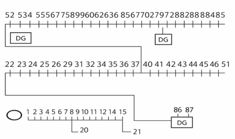
The WAEC 88-Bus radial distribution system in Ikorodu distribution unit was used as test system. The line, load and reliability parameters were collected from Ikorodu business unit and Ikeja distribution company in Nigeria as presented in Appendixes A and B. The sub-station base voltage and MVA values are 11 kV and 15 MVA respectively. The total system active load is 11,654 kW while the total active power loss before DRG integration is 2120 kW with a minimum voltage of 0.9368 p. u at Bus 85. The single line diagram of a simple radial distribution system is presented in Figure 1 while the Single line diagram of 88-Bus WAEC 11 kV radial distribution network with 3-integrated DGs shown in Figure 2. Figure 3 presents the modified cuckoo search optimization computational implementation procedure.
Figure 1. Single line diagram of simple radial distribution system
Figure 2. Single line diagram of 88-Bus WAEC 11 kV radial distribution network with 3-integrted DG
Figure 3. Improved cuckoo search optimization computational implementation procedure
3.2 Problem formulation
In this work, the optimal sizing and location of distributed generation in WAEC-88 Bus radial distribution network is formulated as an objective problem. The main objective function of this research is to minimize the real power loss and improve reliability and voltage profile with DRG integration. Therefore, evaluation of power loss was conducted using BIBC-BCBV matrix method.
In implementation of BFSM Kirchhoff’s current and voltage laws are used. The real and reactive power flowing from Bus ‘i’ to Bus ‘j’ are calculated using Backward direction rule, that is from receiving node to sending node.
The real power flowing is given as
$P_{\mathrm{ij}}=\left(P_{\mathrm{j}}+P_{\mathrm{lj}}\right)+R_{\mathrm{ij}} \frac{\left(P_{\mathrm{j}}+P_{\mathrm{lj}}\right)^2+\left(Q_{\mathrm{j}}+Q_{\mathrm{lj}}\right)^2}{V_{\mathrm{i}}^2}$ (1)
Also, the reactive power flowing is given as
$P_{\mathrm{ij}}=\left(P_{\mathrm{j}}+P_{\mathrm{lj}}\right)+R_{\mathrm{ij}} \frac{\left(P_{\mathrm{j}}+P_{\mathrm{lj}}\right)^2+\left(Q_{\mathrm{j}}+Q_{\mathrm{lj}}\right)^2}{V_{\mathrm{i}}^2}$ (2)
where, $P_{\mathrm{lj}}$ and $Q_{\mathrm{lj}}$ are connected loads at Bus ‘j’.
The forward direction rule was used to calculate the angle and voltage magnitude at each node as follows:
We assume that a voltage $V_{\mathrm{i}}<\emptyset_{\mathrm{i}}$ at Bus ‘i’ and $V_{\mathrm{j}}<\emptyset_{\mathrm{j}}$ at Bus ‘j’ resulted into current ‘í’ and ‘j’ flowing through line ‘N’ with an impedance of $Z_{\mathrm{ij}}=R_{\mathrm{ij}}+X_{\mathrm{ij}}$. Backward forward sweep method was chosen because of its simple computational procedure, fast, high convergence rate and requires less memory compared to the conventional methods. Therefore, the current flowing is calculated thus:
$I_{\mathrm{ij}}=\frac{V_{\mathrm{i}}<\emptyset_{\mathrm{i}}-V_{\mathrm{j}}<\emptyset_{\mathrm{j}}}{R_{\mathrm{ij}}+j X_{\mathrm{ij}}}$ (3)
and
$I_{\mathrm{ij}}=\frac{P_{\mathrm{i}}-Q_{\mathrm{j}}}{V_{\mathrm{i}}<-\emptyset_{\mathrm{i}}}$ (4)
Evaluating Eqs. (3) and (4) above gave the voltage at Bus ‘j’.
$\begin{gathered}V_{\mathrm{j}}=\left[V_{\mathrm{i}}^2-2 \times\left(P_{\mathrm{i}} R_{\mathrm{ij}}+j Q_{\mathrm{i}} X_{\mathrm{ij}}\right)+\left(R_{\mathrm{ij}}^2+X_{\mathrm{ij}}^2\right) \times\right. \\ \left.\left(\frac{P_{\mathrm{i}}^2+Q_{\mathrm{i}}^2}{V_{\mathrm{i}}^2}\right)\right]\end{gathered}$ (5)
Therefore, the power losses per branch between nodes ‘i’ and ‘j’ through ‘N’ line is given as
$P_{\text {loss(ij) }}=R_{\mathrm{ij}} \frac{\left(P_{\mathrm{ij}}^2+Q^2{ }_{\mathrm{ij}}\right)}{V_{\mathrm{j}}^2}$ (6)
$Q_{\text {loss }(\mathrm{ij})}=X_{\mathrm{ij}} \frac{\left(P_{\mathrm{ij}}{ }^2+Q^2{ }_{\mathrm{ij}}\right)}{V_{\mathrm{j}}{ }^2}$ (7)
This implies that the total real and reactive power losses in the distribution network with ‘M’ number of branches can be written as:
$P_{\text {loss }(\mathrm{ij})}=\sum_{j=1}^M P_{\text {loss }(\mathrm{ij})}$ (8)
$Q_{\text {loss(ij) }}=\sum_{j=1}^M Q_{\text {loss(ij) }}$ (9)
The fitness function to minimize the total real power loss is expressed as:
$F=\min \left(P _{\mathrm{L}}=\sum_{i=1}^N I_{\mathrm{i}}^2 R_{\mathrm{i}}\right)$ (10)
where, N is the total number of branches, I is the line current in branch i and R is the resistance of the branches.
The constraints to be satisfied when minimizing the objective function are:
A. Power balance constraint
$\sum P_{\mathrm{DG}}+P_{\text {grid }}=\sum P_{\text {loss }}+P d$ (11)
where, $P_{\text {loss}}$ is the total active power loss in the network, $Pd$ is the active power demand, Pgrid is the active power from utility and $P_{\mathrm{DG}}$ is the active real power generation.
B. Bus constraint
The Bus voltage magnitude must satisfy legal requirement and design limitation restriction limits. Therefore, the voltage magnitude limits are expressed as:
$0.95 \leq V_{\mathrm{i}} \leq 1.0$ (12)
where, 0.95 and 1.0 are the lower and upper voltage Vᵢ at Bus ‘i’.
C. Distributed generation size constraint
Generally, the active power limits of the generator are restricted within a given maximum and minimum limits. Therefore, the DG unit total power limit is expressed as:
$P_{D G}^{\min } \leq P_{\mathrm{DG}} \leq P_{D G}^{\max }$ (13)
where, $P_{\mathrm{DG}}$ is the total power generation of DG units, $P_{DG~}^{min}$ and $P_{DG~}^{max}$ are the lower and upper limits of DG.
D. Reliability indices techniques
The first category is called load point indices or global indices or primary indices, which comprise of average failure rate, λₐ, average outage time, rₐ, and average annual outage time, Uₐ and are expressed mathematically as:
$\lambda_{\mathrm{a}}=\sum_{\mathrm{i}} \lambda_{\mathrm{i}}$ (14)
$U_{\mathrm{a}}=\sum_{\mathrm{i}} \lambda_{\mathrm{i}} r_{\mathrm{i}}$ (15)
$r_{\mathrm{a}}=\frac{\sum_i \lambda i . r_{\mathrm{i}}}{\sum_i \lambda i}$ (16)
The second category is called system indices which are averages that measure every customer’s in the same way. They are generally accepted as reliability measures of worth and often used as reliability benchmarks and for target improvement. These are System Average Interruption Frequency Index (SAIFI), System Average Interruption Duration Index (SAIDI), Customer Average Interruption Duration Index (CAIDI) and Average Service Availability (Unavailability) Index (ASAI) (ASUI). These are expressed mathematically as follows:
$\begin{gathered}S A I F I=\frac{\text { total number of sustained outages per customer }}{\text { total number of served customers }} \\ =\frac{\sum_{\mathrm{i}}\left(\lambda_{\mathrm{i}} \times N_{\mathrm{i}}\right)}{\sum_{\mathrm{i}} N_{\mathrm{i}}}(\text { out } / \text { cust. } \text { yr })\end{gathered}$ (17)
where, λᵢ and Nᵢ are failure rate and number of customers at load point i, respectively. This is used to measure the number of outages an average customer encounter over a period of a year.
$\begin{gathered}S A I D I=\frac{\text { Sum of sustained outages length by a customer }}{\text { total number of served customer }} \\ =\frac{\sum_{\mathrm{i}}\left(U_{\mathrm{i}} x N_{\mathrm{i}}\right)}{\sum_{\mathrm{i}} N_{\mathrm{i}}}(h r / \text { cust. } y r)\end{gathered}$ (18)
where, Uᵢ is annual average time at load point i and Nᵢ stands for number of customers at load point i. This is utilized to evaluate the unavailability of power supply in a year per customer.
$\begin{gathered}C A I D I=\frac{\text { Sum of sustained outages lenght by acustomer }}{\text { total number of customer outages }} \\ =\frac{\sum_{\mathrm{i}}\left(U_{\mathrm{i}} x N_{\mathrm{i}}\right)}{\sum_{\mathrm{i}} \lambda_{\mathrm{i}} .N_{\mathrm{i}}}(h r / c u s t . i n t)\end{gathered}$ (19)
where, Uᵢ, λᵢ and Nᵢ are annual average time, failure rate and number of customers at load point i respectively. This is utilized to ascertain the time taken by the utility during contingencies.
$\begin{gathered}A S A I=\frac{\text { Service available hours to customer }}{\text { customer hours demanded }} \\ =\frac{\sum_{\mathrm{i}} N_{\mathrm{i}} .8760-\sum_{\mathrm{i}} U_{\mathrm{i}} . N_{\mathrm{i}}}{\sum_{\mathrm{i}} N_{\mathrm{i}} .8760}\end{gathered}$ (20)
$\begin{gathered}A S U I=\frac{\text { Service unavailable hours to customer }}{\text { customer hours demanded }} \\ =\frac{\sum_{\mathrm{i}} U_{\mathrm{i}}.N_{\mathrm{i}}}{\sum_{\mathrm{i}} N_{\mathrm{i}} . 8760}\end{gathered}$ (21)
ASAI and ASUI are indices used to calculate power received and not received per customer. When the ASAI value is high, the ASUI value is less and vice visa.
AENS = average energy not supplied
$\begin{gathered}A E N S=\frac{\text { total energy not supplied }}{\text { total number of customer served }} \\ =\frac{\sum_{\mathrm{i} E E N_{\mathrm{i}}}}{\sum_{\mathrm{i}} N_{\mathrm{i}}}(k W h r / c u s t . y r)\end{gathered}$ (22)
3.3 Improved cuckoo search method
3.3.1 Cuckoo search technique
Cuckoo search technique (CST) is a simulation of random walk processes of cuckoo species searching for suitable host next to lay their eggs. This is proposed by Yang and Deb [28]. It is a population-based algorithm with simple procedure and less control parameters. There are specified principles to be followed when using cuckoo search algorithm in solving optimization problems. These principles are:
Levy flights random walk and selective random walk are used by cuckoo in laying their eggs in host nests. Levy flight is a random walk used to generate new solution and can be expressed mathematically as:
$S_{\mathrm{i}}^{\mathrm{t}+1}=S_{\mathrm{i}}^{\mathrm{t}}+\alpha \otimes \operatorname{Lev} y(\beta)$ (23)
where, $\alpha ~$denotes change of position and is expressed as:
$\alpha=\alpha^0 \times c \times\left(S_{\mathrm{i}}^{\mathrm{t}}-S_{\mathrm{best}}\right)$ (24)
where, ${{\alpha }^{0}}$ is the scaling factor with an assigned value of 0.1.$S_{\mathrm{b}_{\mathrm{est}}}$ represents the global best solution so far obtained and c represents a random step size generated with the help of Levy distribution and is expressed as:
$c=\frac{\mathrm{U}}{|v|^{1 / \beta}}$ (25)
Therefore, substituting Eqs. (24) and (25) in Eq. (23) we have
$S_{\mathrm{i}}^{\mathrm{t}+1}=S_{\mathrm{i}}^{\mathrm{t}}+\alpha^0\left(\frac{\mathrm{u}}{|v|^{\frac{1}{\beta}}}\right)\left(S_{\mathrm{i}}^{\mathrm{t}}-S_{\mathrm{b}_{\mathrm{est}}}\right)$ (26)
$u=randn~\left( size~\left( s \right) \right)*\sigma $ (27)
$v=randn~\left( size~\left( s \right) \right)$ (28)
where, the sigma function$~\sigma $ is expressed as
$\sigma_{\mathrm{u}}=\left(\frac{\left(\Gamma(1+\beta) \times \sin \left(\pi \times \frac{\beta}{2}\right)\right.}{\Gamma\left(\frac{1+\beta}{2}\right) \times \beta \times 2^{(\beta-2) / 2}}\right)^{1 / \beta}$ (29)
β is a constant and usually set to a value of 1.5. Г represents a gamma distribution and u and v are random numbers from normal distribution. In implementing cuckoo search algorithm these have values attached as shown in Eqs. (20) and (21).
Probability based random walk
This is usually used to detect the new global best. Here, current best is considered as a base vector with two different solutions which are randomly selected then the new global solution is determined through probability formulations. That is
If r < Pa then
$S_{i, m}^{t+1}=S_{i, m}^t+\operatorname{rand}\left(S_{p, m}^t-S_{q, m}^t\right)$ (30)
If not, we have
$S_{i, m}^{t+1}=S_{i, m}^t$ (31)
where, p and q are random integer numbers and m represents mth dimension of solution while rand is random number in the range of (0,1) and Pa is fractional probability.
3.3.2 Accuracy and convergence rate
Cuckoo search technique was improved to increase the efficiency, that is enhancing the accuracy and the converging rate of the system. Two modifications are made one on levy flight step size and the second on addition of information exchange between two groups of top eggs formulated. The value of step size in CS is one while in ICSA the step size value decreases as the number of generations increases resulting in increase in localized searching between the eggs or DRGs. Therefore, performing levy flight on nest or network Sᵢᵗ and generating new egg or DRG or solution Sᵢᵗ+1 while distancing the worst nest or DRG from the best nest or DRG using the modified equation:
$\begin{gathered}S_{\mathrm{i}}^{\mathrm{t}+1}=\operatorname{round}\left(S_{\mathrm{i}}^{\mathrm{t}}+0.01 *\left(\frac{u}{|V|^{1^{\prime} \beta}}\right) *\left(S_{\mathrm{i}}^{\mathrm{t}}-\right.\right. \left.\left.S_{\mathrm{i}}^{\mathrm{t}} \text { best }\right) * \operatorname{randn}\left(\operatorname{size}\left(S_{\mathrm{i}}^{\mathrm{t}}\right)\right)\right)+D / N I^2\end{gathered}$ (32)
where,
$u=randn(size\left( s \right)*\sigma $ (33)
$\text{v}=randn(size\left( s \right)$ (34)
$\sigma_{\mathrm{u}}=\left(\frac{\left(\Gamma(1+\beta) \times \sin \left(\pi \times \frac{\beta}{2}\right)\right.}{\Gamma\left(\frac{1+\beta}{2}\right) \times \beta \times 2^{(\beta-2) / 2}}\right)^{1 / \beta}$ (35)
We move a distance = $\left|S_{\mathrm{i}}^{\mathrm{t}}-S_{\mathrm{j}}^{\mathrm{t}}\right| / 0.1$ from worst nest to best nest to find the new solution expressed as
$S_{\mathrm{i}}{ }^{\mathrm{t}+1}=S_{\mathrm{i}}{ }^{\mathrm{t}}$ worst $+\frac{\left|S_{\mathrm{i}}^{\mathrm{t}}-S_{\mathrm{j}}^{\mathrm{t}}\right|}{0.1}$ (36)
In order to achieve the aim of this study, the outage data from WAEC distribution network in Ikorodu Business unit was collected using quantitative method. The reliability status of the network was determined to ascertain its healthiness through load flow analysis after data collected was processed and analysed using backward-forward sweep method for load flow analysis. The improved cuckoo search algorithm was employed for DRG integration at optimal location and size in the distribution network. Cuckoo search algorithm toolbox which was coded in MATLAB generated both optimal distributed renewable generation size and site as outputs. The size and site generated as outputs for 2DRG and 3DRG were integrated separately in the distribution network Figure 2 using Eq. (27) with computational procedure of Figure 3 in MATLAB software environment. The optimal 2-DRGs location and size are Bus 88 with 1000 kW and Bus 70 with 1000 kW. Also, the optimal 3-DGs location and size are Bus 88 with 1000 kW, Bus 76 with 1000 kW and Bus 53 with 1000 kW. Thereafter, the reliability indices values were calculated using Eqs. (10)-(15).
The following parameter are set prior to starting:
NBus_Min=2, NBus_Max=88,
DG_Size_Min=10, DG_Size_Max =1000,
Max_Iter=20, Initial Step_Size =2.
The results of the design system, tested on WAEC distribution network using backward/forward sweep method in MATLAB environment for determining load flow and reliability values at base case is in Table 1.
Table 1. Load flow and reliability result at base case
|
S/N |
Parameter |
Base Case Value |
|
1 |
Power loss (kW) |
2120.3437 |
|
2 |
Optimal DG location |
NIL |
|
3 |
Optimal DG size P Kw |
NIL |
|
4 |
Optimal DG size Q kVar |
NIL |
|
5 |
Total DG |
NIL |
|
6 |
Voltage Minimum @ Bus No. |
0.93682 @ 85 |
|
7 |
Voltage Maximum @ Bus No. |
1 @ 1 |
|
8 |
Execution Time (seconds) |
4.4708 |
|
9 |
SAIDI (hr / c. yr) |
38.2089 |
|
10 |
SAIFI (f / c. yr) |
10.9019 |
|
11 |
EENS (MWhr / yr) |
183,168.2429 |
|
12 |
AENS (MWhr / c. yr) |
3.287 |
|
13 |
ASAI (p. u) |
0.99564 |
|
14 |
ASUI (p. u) |
0.0043617 |
|
15 |
CAIDI (hr / c. int.) |
3.5048 |
The cuckoo search algorithm toolbox coded in MATLAB generated both optimal distributed renewable generation size and site as output. The size and site generated as outputs for 2DRG and 3DRG were integrated separately on the distribution network given the results as shown in Table 2.
Table 2. Load flow and reliability result for 2 integrated DRGs
|
S/N |
Parameter |
DG Placement Values |
|
1 |
Power loss (kW) |
1243.9609 |
|
2 |
Optimal DG location |
80, 70 |
|
3 |
Optimal DG size P Kw |
1000, 1000 |
|
4 |
Optimal DG size Q kVar |
750, 750 |
|
5 |
Total DG |
2000 |
|
6 |
Voltage Minimum @ Bus No. |
0.95191 @ 85 |
|
7 |
Voltage Maximum @ Bus No. |
1 @ 1 |
|
8 |
Execution Time (seconds) |
600.702 |
|
9 |
SAIDI (hr / c. yr) |
29.8699 |
|
10 |
SAIFI (f / c. yr) |
10.8163 |
|
11 |
EENS (MWhr / yr) |
156,599.553 |
|
12 |
AENS (MWhr / c. yr) |
2.8102 |
|
13 |
ASAI (p. u) |
0.99659 |
|
14 |
ASUI (p. u) |
0.0034098 |
|
15 |
CAIDI (hr / c. int.) |
2.7616 |
Table 3. Load flow and reliability result for 3 integrated DRGs
|
S/N |
Parameter |
DG Placement Values |
|
1 |
Power loss (kW) |
926.5949 |
|
2 |
Optimal DG location |
88, 76, 53 |
|
3 |
Optimal DG size P Kw |
1000, 1000, 1000 |
|
4 |
Optimal DG size Q kVar |
750, 750, 750 |
|
5 |
Total DG |
3000 |
|
6 |
Voltage Minimum @ Bus No. |
0.95924 @ 85 |
|
7 |
Voltage Maximum @ Bus No. |
1 @ 1 |
|
8 |
Execution Time (seconds) |
1395.1822 |
|
9 |
SAIDI (hr / c. yr) |
29.4375 |
|
10 |
SAIFI (f / c. yr) |
10.7622 |
|
11 |
EENS (MWhr / yr) |
153,798.1488 |
|
12 |
AENS (MWhr / c. yr) |
2.7599 |
|
13 |
ASAI (p. u) |
0.99664 |
|
14 |
ASUI (p. u) |
0.0033604 |
|
15 |
CAIDI (hr / c. int.) |
2.7353 |
The data collected was analysed automatically while the data collated was analysed sequentially using percentages and result interpreted graphically using MATLAB software.
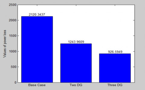
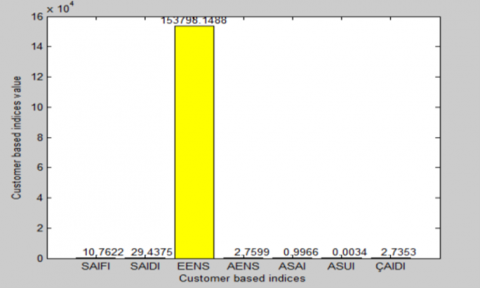
The DRGs integration, their corresponding sizes, power loss, voltage per unit and reliability indices with and without DRGs using improved cuckoo search algorithm (ICSA) and backward/forward sweep algorithm (BFSA) in Matlab software environment are summarized in Tables 1-3. The minimum voltage value reached at base level was 0.9368 per unit at Bus number 85 but after integration of 2DG at Buses 88 and 70, the power loss reduced from 2120.3437 to 1243.9609 kW which is 41.36% power loss reduction with much improvement recorded in reliability indices at minimum voltage value of 0.9519 per unit at Bus number 85. Also, with 3DG integrated the power loss further reduced to 926.5949 kW from 2120.3437 kW which is 56.30% power loss reduction from the base value while far more improvement was reached in reliability indices with minimum voltage value of 0.9592 per unit at Bus number 85. The trend of improvement in voltage profile are shown in Figures 4-6, while Figure 7 shows a higher power loss reduction with 3DG integration. In addition, the graph of customer-oriented indices is shown in Figures 8-10.
Figure 4. Voltage magnitude of Buses without DREGs injection
Figure 5. Voltage magnitude of Buses with 2-DREG injection
Figure 6. Voltage magnitude of Buses with 3DRGs injection
Figure 7. Comparison of power loss with or without DGs
Figure 8. Graph of customer-oriented indices without DRG
Figure 9. Graph of customer-oriented indices with 2-DRG integrated
Figure 10. Graph of customer-oriented indices with 3-DRG integrated
Furthermore, the increase in number of DRGs integration will bring the ASAI value close to reliability standard value of 0.999999999 p.u. Moreover, reduction in power loss and improvement in voltage level signified more power availability to the consumers and more stable voltage. In Table 4 with 2DG and 3DG integration, the percentage decrease in 2DG for SAIFI, SAIDI, CAIDI and ASUI are 0.79%, 21.82%, 21.21% and 21.82% respectively, and for 3DG integrated, the percentage decrease in reliability indices for SAIFI, SAIDI, CAIDI and ASUI values are 1.28%, 22.96%, 21.96% and 22.96% respectively and are consequently depicted graphically in Figures 11 and 12. Moreover, Reduction in reliability indices values signified maintaining continuity of power supply to the consumers. In Table 5, the comparison of base case parameters with DRG placement is presented while in Table 6, ICSA is compared with CSA.
Figure 11. Comparison of reliability indices before and after 2DRGs injection
Figure 12. Comparison of reliability indices before and after 3DRGs injection
Table 4. Comparison of reliability indices before and after injection of 2DRG and 3DRG (ICSA)
|
Index |
Before DRG |
After Two DRG |
% Decrease |
After Three DRG |
% Decrease |
|
SAIFI |
10.9019 |
10.8163 |
0.79 |
10.7622 |
1.28 |
|
SAIDI |
38.2089 |
29.8699 |
21.82 |
29.4375 |
22.96 |
|
CAIDI |
3.5048 |
2.7616 |
21.21 |
2.7353 |
21.96 |
|
ASUI |
4.3617E-3 |
3.4098E-3 |
21.82 |
3.3604E-3 |
22.96 |
Table 5. Comparison of base case parameters with DRG placement
|
S/N |
Parameter |
Base Case Value |
2DG Placement |
3DG Placement |
|
1 |
Power loss (kW) |
2120.3437 |
1243.9609 |
926.5949 |
|
2 |
Optimal DG location |
NIL |
88, 70 |
88, 76, 53 |
|
3 |
Optimal DG size P Kw |
NIL |
1000, 1000 |
1000, 1000, 1000 |
|
4 |
Optimal DG size Q kVar |
NIL |
750, 750 |
750, 750, 750 |
|
5 |
Total DG |
NIL |
2000 |
3000 |
|
6 |
Voltage Minimum @ Bus No. |
0.93682 @ 85 |
0.95191 @ 85 |
0.95924 @ 85 |
|
7 |
Voltage Maximum @ Bus No. |
1 @ 1 |
1 @ 1 |
1 @ 1 |
|
8 |
Execution Time (seconds) |
4.4708 |
600.702 |
1395.1822 |
|
9 |
SAIDI (hr / c. yr) |
38.2089 |
29.8699 |
29.4375 |
|
10 |
SAIFI (f / c. yr) |
10.9019 |
10.8163 |
10.7622 |
|
11 |
EENS (MWhr / yr) |
183,168.2429 |
156,599.553 |
153,798.1488 |
|
12 |
AENS (MWhr / c. yr) |
3.287 |
2.8102 |
2.7599 |
|
13 |
ASAI (p. u) |
0.99564 |
0.99659 |
0.99664 |
|
14 |
ASUI (p. u) |
0.0043617 |
0.0034098 |
0.0033604 |
|
15 |
CAIDI (hr / c. int.) |
3.5048 |
2.7616 |
2.7353 |
Table 6. Comparison of base case, CSA and ICSA for validation
|
S/N |
Parameter |
Base Case Value |
2DG CSA |
2DG ICSA |
3DG CSA |
3DG ICSA |
|
1 |
Power loss (kW) |
2120.3437 |
1271.80 |
1243.9609 |
970.6 |
926.5949 |
|
2 |
Optimal DG location |
NIL |
69, 51 |
88, 70 |
84, 58, 65 |
88, 76, 53 |
|
3 |
Optimal DG size P Kw |
NIL |
597, 1000 |
1000, 1000 |
564, 1000, 1000 |
1000, 1000, 1000 |
|
4 |
Optimal DG size Q kVar |
NIL |
717.75, 750 |
750, 750 |
423, 750, 750 |
750, 750, 750 |
|
5 |
Total DG |
NIL |
1597 |
2000 |
2564 |
3000 |
|
6 |
Voltage Minimum @ Bus No. |
0.93682 @ 85 |
0.95133 @ 85 |
0.95191 @ 85 |
0.95899@83 |
0.95924 @ 85 |
|
7 |
Voltage Maximum @ Bus No. |
1 @ 1 |
1 @ 1 |
1 @ 1 |
1 @ 1 |
1 @ 1 |
|
8 |
Execution Time (seconds) |
4.4708 |
205.711 |
600.702 |
206.143 |
1395.1822 |
|
9 |
SAIDI (hr / c. yr) |
38.2089 |
38.1094 |
29.8699 |
37.1457 |
29.4375 |
|
10 |
SAIFI (f / c. yr) |
10.9019 |
10.896 |
10.8163 |
10.7834 |
10.7622 |
|
11 |
EENS (MWhr / yr) |
183,168.2429 |
182574.5586 |
156,599.553 |
175219.20 |
153,798.1488 |
|
12 |
AENS (MWhr / c. yr) |
3.287 |
3.2763 |
2.8102 |
3.1444 |
2.7599 |
|
13 |
ASAI (p. u) |
0.99564 |
0.99565 |
0.99659 |
0.99576 |
0.99664 |
|
14 |
ASUI (p. u) |
0.0043617 |
0.0043504 |
0.0034098 |
0.0042404 |
0.0033604 |
|
15 |
CAIDI (hr / c. int.) |
3.5048 |
3.4976 |
2.7616 |
3.4447 |
2.7353 |
In conclusion, the viability of this design system was first tested on WAEC distribution network using Backward-Forward sweep method in MATLAB 2021 software environment for achieving the reliability enhancement. The ICSA provides both optimal location and sizing of DRGs as outputs. It is also demonstrated that the proposed method is capable of reducing power loss, reliability indices: SAIFI, SAIDI, CAIDI, EENS, AENS and ASAI coupled with improvement in ASUI and voltage profile by comparing the results before and after optimization in a real and large Nigeria distribution network. The study recommends further study on Impact of DRGs auxiliary components degradation, detailed reliability cost, economics studies, cost benefit analysis and worth analysis in distribution network.
The authors wish to acknowledge Covenant University for her support in the completion of this study.
|
MRBTS |
Modified Roy Billington Test System |
|
SDGs |
Sustainable Development Goals |
|
DRG |
Distributed Renewable Generation |
|
ESST |
Energy Storage System Technology |
|
SHP |
Small Hydro Power |
|
CST |
Cuckoo Search Technique |
|
CSA |
Cuckoo Search Algorithm |
|
WAMPAC |
Wide Area Monitoring, Protection and Control |
|
PV |
Photovoltaic |
|
FACTS |
Flexible AC Transmission Systems |
|
IEA |
International Energy |
|
EIA |
U.S. Energy Information Administration |
|
WHC |
World Hydro Power Congress |
|
ETAP |
Electrical Transient Analyzer Program |
|
MCSA |
Modified Cuckoo Search Algorithm |
|
KV |
Kilovolts |
|
MVA |
Megavolts-ampere |
|
MW |
Megawatts |
|
Pu |
Per unit |
|
P |
Active Power |
|
Q |
Reactive Power |
|
R |
Line resistance |
|
|V| |
Voltage magnitude |
|
X |
Line reactance |
|
Z |
Line impedance |
|
$V_s$ |
Sending end voltage |
|
$V_r$ |
Receiving end voltage |
|
$\delta$ |
Angle difference between sending and receiving end voltage |
Appendix A
Line Information of WAEC Channel Feeder
|
LINE S/N |
Sending End |
Receiving End |
Resistance (ohm) |
Reactance (ohm) |
|
1 |
1 |
2 |
0.0089 |
0.0098 |
|
2 |
2 |
3 |
0.0085 |
0.0141 |
|
3 |
3 |
4 |
0.0090 |
0.0149 |
|
4 |
4 |
5 |
0.0105 |
0.0750 |
|
5 |
5 |
6 |
0.0036 |
0.0059 |
|
6 |
6 |
7 |
0.0056 |
0.0093 |
|
7 |
7 |
8 |
0.0095 |
0.0157 |
|
8 |
8 |
9 |
0.0052 |
0.0087 |
|
9 |
9 |
10 |
0.0088 |
0.0145 |
|
10 |
10 |
11 |
0.0047 |
0.0077 |
|
11 |
11 |
12 |
0.0074 |
0.0122 |
|
12 |
12 |
13 |
0.0055 |
0.0091 |
|
13 |
13 |
14 |
0.0066 |
0.0120 |
|
14 |
14 |
15 |
0.0069 |
0.0115 |
|
15 |
15 |
16 |
0.0079 |
0.0131 |
|
16 |
16 |
17 |
0.0087 |
0.0143 |
|
17 |
17 |
18 |
0.0042 |
0.0069 |
|
18 |
18 |
19 |
0.0100 |
0.0176 |
|
19 |
9 |
20 |
0.0096 |
0.0142 |
|
20 |
18 |
21 |
0.0145 |
0.0239 |
|
21 |
16 |
22 |
0.0055 |
0.0091 |
|
22 |
22 |
23 |
0.0058 |
0.0096 |
|
23 |
23 |
24 |
0.0054 |
0.0089 |
|
24 |
24 |
25 |
0.0062 |
0.0102 |
|
25 |
25 |
26 |
0.0091 |
0.0151 |
|
26 |
26 |
27 |
0.0078 |
0.0129 |
|
27 |
27 |
28 |
0.0055 |
0.0092 |
|
28 |
28 |
29 |
0.0105 |
0.0173 |
|
29 |
29 |
30 |
0.0119 |
0.0196 |
|
30 |
30 |
31 |
0.0197 |
0.0327 |
|
31 |
31 |
32 |
0.0098 |
0.0327 |
|
32 |
32 |
33 |
0.0066 |
0.0109 |
|
33 |
33 |
34 |
0.0055 |
0.0091 |
|
34 |
34 |
35 |
0.0050 |
0.0085 |
|
35 |
35 |
36 |
0.0056 |
0.0092 |
|
36 |
36 |
37 |
0.0083 |
0.0137 |
|
37 |
37 |
38 |
0.0065 |
0.0107 |
|
38 |
38 |
39 |
0.0063 |
0.0105 |
|
39 |
39 |
40 |
0.0063 |
0.0104 |
|
40 |
40 |
41 |
0.0072 |
0.0119 |
|
41 |
41 |
42 |
0.0074 |
0.0122 |
|
42 |
42 |
43 |
0.0091 |
0.0151 |
|
43 |
43 |
44 |
0.0119 |
0.0198 |
|
44 |
44 |
45 |
0.0090 |
0.0149 |
|
45 |
45 |
46 |
0.0057 |
0.0094 |
|
46 |
46 |
47 |
0.0065 |
0.0101 |
|
47 |
47 |
48 |
0.0094 |
0.0153 |
|
48 |
48 |
49 |
0.0071 |
0.0118 |
|
49 |
49 |
50 |
0.0077 |
0.0128 |
|
50 |
50 |
51 |
0.0076 |
0.0126 |
|
51 |
40 |
52 |
0.0051 |
0.0085 |
|
52 |
52 |
53 |
0.0098 |
0.0162 |
|
53 |
53 |
54 |
0.0106 |
0.0175 |
|
54 |
54 |
55 |
0.0081 |
0.0135 |
|
55 |
55 |
56 |
0.0050 |
0.0083 |
|
56 |
56 |
57 |
0.0132 |
0.0218 |
|
57 |
57 |
58 |
0.0085 |
0.0140 |
|
58 |
58 |
59 |
0.0079 |
0.0131 |
|
59 |
59 |
60 |
0.0108 |
0.0179 |
|
60 |
60 |
61 |
0.0095 |
0.0157 |
|
61 |
61 |
62 |
0.0018 |
0.0195 |
|
62 |
62 |
63 |
0.0065 |
0.0108 |
|
63 |
63 |
64 |
0.0078 |
0.0121 |
|
64 |
64 |
65 |
0.0135 |
0.0223 |
|
65 |
65 |
66 |
0.0101 |
0.0167 |
|
66 |
66 |
67 |
0.0072 |
0.0119 |
|
67 |
67 |
68 |
0.0042 |
0.0070 |
|
68 |
68 |
69 |
0.0049 |
0.0080 |
|
69 |
69 |
70 |
0.0094 |
0.0156 |
|
70 |
70 |
71 |
0.0127 |
0.0211 |
|
71 |
71 |
72 |
0.0131 |
0.0217 |
|
72 |
72 |
73 |
0.0148 |
0.0245 |
|
73 |
73 |
74 |
0.0095 |
0.0158 |
|
74 |
74 |
75 |
0.0069 |
0.0115 |
|
75 |
75 |
76 |
0.0081 |
0.0133 |
|
76 |
76 |
77 |
0.0068 |
0.0113 |
|
77 |
77 |
78 |
0.0097 |
0.0160 |
|
78 |
78 |
79 |
0.0077 |
0.0127 |
|
79 |
79 |
80 |
0.0055 |
0.0091 |
|
80 |
80 |
81 |
0.0069 |
0.0115 |
|
81 |
81 |
82 |
0.0065 |
0.0108 |
|
82 |
82 |
83 |
0.0081 |
0.0134 |
|
83 |
83 |
84 |
0.0145 |
0.0241 |
|
84 |
84 |
85 |
0.0041 |
0.0069 |
|
85 |
40 |
86 |
0.0104 |
0.0172 |
|
86 |
86 |
87 |
0.0128 |
0.0211 |
|
87 |
87 |
88 |
0.0073 |
0.0120 |
Appendix B
Reliability Data Information of WAEC Distribution Feeder
|
LINE S/N |
Sending End |
Receiving End |
Outage Rate (f/yr) |
Repair Time (hrs) |
Customers Number |
|
1 |
1 |
2 |
0.0360 |
1.50 |
1500 |
|
2 |
2 |
3 |
0.2800 |
0.90 |
1000 |
|
3 |
3 |
4 |
0.2100 |
8.90 |
1000 |
|
4 |
4 |
5 |
0.0190 |
3.22 |
750 |
|
5 |
5 |
6 |
0.4000 |
2.00 |
950 |
|
6 |
6 |
7 |
0.1750 |
3.11 |
950 |
|
7 |
7 |
8 |
0.9000 |
2.75 |
950 |
|
8 |
8 |
9 |
0.4400 |
2.44 |
300 |
|
9 |
9 |
10 |
0.0205 |
1.60 |
350 |
|
10 |
10 |
11 |
0.8000 |
3.05 |
500 |
|
11 |
11 |
12 |
0.3100 |
1.00 |
450 |
|
12 |
12 |
13 |
0.4500 |
4.10 |
300 |
|
13 |
13 |
14 |
0.0269 |
1.50 |
400 |
|
14 |
14 |
15 |
0.3600 |
1.50 |
325 |
|
15 |
15 |
16 |
0.6600 |
0.50 |
350 |
|
16 |
16 |
17 |
0.4400 |
2.11 |
1500 |
|
17 |
17 |
18 |
0.0320 |
3.12 |
1300 |
|
18 |
18 |
19 |
0.0210 |
1.80 |
1300 |
|
19 |
9 |
20 |
0.9400 |
6.50 |
350 |
|
20 |
18 |
21 |
0.1700 |
3.44 |
300 |
|
21 |
16 |
22 |
0.2500 |
2.70. |
450 |
|
22 |
22 |
23 |
0.3300 |
2.35 |
400 |
|
23 |
23 |
24 |
0.1200 |
3.50 |
325 |
|
24 |
24 |
25 |
0.1045 |
4.30 |
500 |
|
25 |
25 |
26 |
0.5100 |
2.22 |
350 |
|
26 |
26 |
27 |
0.2300 |
2.80 |
550 |
|
27 |
27 |
28 |
0.5091 |
3.25 |
450 |
|
28 |
28 |
29 |
0.4110 |
3.27 |
400 |
|
29 |
29 |
30 |
0.2100 |
4.40 |
350 |
|
30 |
30 |
31 |
0.7000 |
2.11 |
350 |
|
31 |
31 |
32 |
0.6300 |
2.05 |
350 |
|
32 |
32 |
33 |
0.0160 |
3.15 |
375 |
|
33 |
33 |
34 |
0.1900 |
2.70 |
475 |
|
34 |
34 |
35 |
0.0405 |
3.55 |
550 |
|
35 |
35 |
36 |
0.3000 |
4.10 |
600 |
|
36 |
36 |
37 |
0.1000 |
2.80 |
650 |
|
37 |
37 |
38 |
0.1800 |
2.35 |
350 |
|
38 |
38 |
39 |
0.2100 |
3.22 |
400 |
|
39 |
39 |
40 |
0.2300 |
3.45 |
400 |
|
40 |
40 |
41 |
0.5100 |
2.80 |
400 |
|
41 |
41 |
42 |
0.7700 |
2.75 |
550 |
|
42 |
42 |
43 |
0.4100 |
4.00 |
350 |
|
43 |
43 |
44 |
0.1400 |
2.45 |
350 |
|
44 |
44 |
45 |
0.3900 |
2.12 |
450 |
|
45 |
45 |
46 |
0.4400 |
3.05 |
450 |
|
46 |
46 |
47 |
0.2500 |
2.46 |
300 |
|
47 |
47 |
48 |
0.1045 |
8.50 |
350 |
|
48 |
48 |
49 |
0.8000 |
2.75 |
550 |
|
49 |
49 |
50 |
0.4000 |
6.25 |
475 |
|
50 |
50 |
51 |
0.3100 |
3.05 |
350 |
|
51 |
40 |
52 |
0.1700 |
2.07 |
300 |
|
52 |
52 |
53 |
0.3100 |
3.11 |
700 |
|
53 |
53 |
54 |
0.2800 |
2.33 |
900 |
|
54 |
54 |
55 |
0.3100 |
3.33 |
1000 |
|
55 |
55 |
56 |
0.6600 |
2.90 |
350 |
|
56 |
56 |
57 |
0.3300 |
2.30 |
400 |
|
57 |
57 |
58 |
0.7000 |
3.60 |
500 |
|
58 |
58 |
59 |
0.4300 |
3.99 |
500 |
|
59 |
59 |
60 |
0.0900 |
2.70 |
450 |
|
60 |
60 |
61 |
0.6000 |
4.10 |
450 |
|
61 |
61 |
62 |
0.3400 |
2.40 |
400 |
|
62 |
62 |
63 |
0.2500 |
2.60 |
400 |
|
63 |
63 |
64 |
0.6100 |
3.06 |
1200 |
|
64 |
64 |
65 |
0.1100 |
3.40 |
1300 |
|
65 |
65 |
66 |
0.1679 |
2.72 |
1000 |
|
66 |
66 |
67 |
0.1045 |
6.70 |
1300 |
|
67 |
67 |
68 |
0.3400 |
3.05 |
400 |
|
68 |
68 |
69 |
0.1750 |
2.45 |
350 |
|
69 |
68 |
71 |
0.1700 |
2.55 |
1500 |
|
70 |
71 |
72 |
0.2000 |
2.80 |
1300 |
|
71 |
72 |
73 |
0.4000 |
3.10 |
1200 |
|
72 |
73 |
74 |
0.5500 |
3.98 |
1300 |
|
73 |
74 |
75 |
0.0220 |
3.43 |
900 |
|
74 |
75 |
76 |
0.1200 |
3.75 |
650 |
|
75 |
76 |
77 |
0.6100 |
2.11 |
400 |
|
76 |
77 |
78 |
0.1700 |
2.04 |
350 |
|
77 |
78 |
79 |
0.0400 |
3.46 |
900 |
|
78 |
79 |
80 |
0.5000 |
2.22 |
350 |
|
79 |
80 |
81 |
0.3600 |
2.70 |
300 |
|
80 |
81 |
82 |
0.0230 |
3.15 |
900 |
|
81 |
82 |
83 |
0.0800 |
4.10 |
300 |
|
82 |
83 |
84 |
0.9200 |
3.22 |
350 |
|
83 |
84 |
85 |
0.3700 |
4.12 |
900 |
|
84 |
40 |
86 |
0.2400 |
2.90 |
650 |
|
85 |
86 |
87 |
0.5000 |
2.77 |
1300 |
|
86 |
87 |
88 |
0.6500 |
3.37 |
1300 |
[1] Ehimen, A.A., Simon, I.N. (2020). Reliability prediction in the Nigerian power industry using neural network. Journal of Electrical and Electronics Engineering, 13(2): 17-22.
[2] Aıroboman, A. (2022). Forecasting of maximum peak load demand of Abuja region interconnected power network using artificial neural network. International Journal of Engineering Science and Application, 6(1): 12-28.
[3] Ibrahim, S.O., Abel, A. (2020). A study on the optimal location of injection substation in Nigeria: A review. In 2020 6th IEEE International Energy Conference (ENERGYCon), Gammarth, Tunisia, pp. 808-812. https://doi.org/10.1109/ENERGYCon48941.2020.9236482
[4] Aligbe, A., Airoboman, A.E., Uyi, A.S., Orukpe, P.E. (2021). Microgrid, its control and stability: The state of the art. International Journal of Emerging Scientific Research, 3: 1-12. https://doi.org/10.37121/ijesr.v3.145
[5] Adoghe, A.U., Adeyemi-Kayode, T.M., Oguntosin, V., Amahia, I.I. (2023). Performance evaluation of the prospects and challenges of effective power generation and distribution in Nigeria. Heliyon, 9(3): e14416. https://doi.org/10.1016/j.heliyon.2023.e14416
[6] Gautam, P., Karki, R. (2018). Quantifying reliability contribution of an energy storage system to a distribution system. In 2018 IEEE Power & Energy Society General Meeting (PESGM), Portland, OR, USA, pp. 1-5. https://doi.org/10.1109/PESGM.2018.8586222
[7] Aderibigbe, M.A., Adoghe, A.U., Agbetuyi, F., Airoboman, A.E. (2021). A review on optimal placement of distributed generators for reliability improvement on distribution network. In 2021 IEEE PES/IAS Power Africa, Nairobi, Kenya, pp. 1-5. https://doi.org/10.1109/PowerAfrica52236.2021.9543266
[8] Adefarati, T., Bansal, R.C. (2017). Reliability assessment of distribution system with the integration of renewable distributed generation. Applied Energy, 185: 158-171. https://doi.org/10.1016/j.apenergy.2016.10.087
[9] Ahmad, S., Asar, A.U. (2021). Reliability enhancement of electric distribution network using optimal placement of distributed generation. Sustainability, 13(20): 11407. https://doi.org/10.3390/su132011407
[10] Escalera, A., Hayes, B., Prodanovic, M. (2017). Analytical method to assess the impact of distributed generation and energy storage on reliability of supply. CIRED, 2017(1): 2092-2096. https://doi.org/10.1049/oap-cired.2017.1106
[11] Ndawula, M.B., Djokic, S.Z., Hernando-Gil, I. (2019). Reliability enhancement in power networks under uncertainty from distributed energy resources. Energies, 12(3): 531. https://doi.org/10.3390/en12030531
[12] Badr, A.A., Kalantari, N.T. (2017). Reliability evaluation of radial distribution systems including distributed generation based on an improved classification algorithm. UPB Scientific Bulletin, Series C, 79(4): 211-228.
[13] Mahmoud, M., Elshahed, M., Elsobki, M. (2018). The impact of distributed energy resources on the reliability of smart distribution system. Majlesi Journal of Electrical Engineering, 12(4): 1-14.
[14] Gana, M., Dalyop, I., Mustapha, M., Maxwell, J.C. (2020). Assessment of reliability of distribution network with embedded generation. International Journal of Electrical and Electronics Engineering, 7(2): 34-37.
[15] Enyew, B.M., Salau, A.O., Khan, B., Hagos, I.G., Takele, H., Osaloni, O.O. (2023). Techno-Economic analysis of distributed generation for power system reliability and loss reduction. International Journal of Sustainable Energy, 42(1): 873-888. https://doi.org/10.1080/14786451.2023.2244617
[16] Ghosh, D. (2020). Impact of distributed generation on the reliability allocation of distribution system: A mesh-grid approach. In 2020 International Conference on Emerging Frontiers in Electrical and Electronic Technologies (ICEFEET), Patna, India, pp. 1-6. https://doi.org/10.1109/ICEFEET49149.2020.9187019
[17] Ghaedi, A., Mirzadeh, M. (2020). The impact of tidal height variation on the reliability of barrage-type tidal power plants. International Transactions on Electrical Energy Systems, 30(9): e12477. https://doi.org/10.1002/2050-7038.12477
[18] Agbetuyi, A.F., Ademola, A., Orovwode, H.E., Oladipupo, O.K., Simeon, M., Agbetuyi, O.A. (2021). Power quality considerations for embedded generation integration in Nigeria: A case study of OGBA 33 kV injection substation. International Journal of Electrical and Computer Engineering, 11(2): 956-965. http//doi.org/10.11591/ijece.v11i2.pp956-965
[19] Ogunsina, A.A., Petinrin, M.O., Petinrin, O.O., Offornedo, E.N., Petinrin, J.O., Asaolu, G.O. (2021). Optimal distributed generation location and sizing for loss minimization and voltage profile optimization using ant colony algorithm. SN Applied Sciences, 3(2): 248. https://doi.org/10.1007/s42452-021-04226-y
[20] Airoboman, A.E., Salihu, H., Araga, I.A. (2022). Optimal siting and sizing of capacitor for voltage profile and efficiency enhancement in a transmission system with N-1 contingency. Nigerian Journal of Engineering, 29(3): 48-61.
[21] Ahmadi, B., Ceylan, O., Ozdemir, A. (2019). Cuckoo search algorithm for optimal siting and sizing of multiple distributed generators in distribution grids. In 2019 Modern Electric Power Systems (MEPS), Wroclaw, Poland, pp. 1-6. https://doi.org/10.1109/MEPS46793.2019.9395018
[22] Reddy P, D.P., Reddy V.C., V., Manohar T., G. (2018). Ant Lion optimization algorithm for optimal sizing of renewable energy resources for loss reduction in distribution systems. Journal of Electrical Systems and Information Technology, 5(3): 663-680. https://doi.org/10.1016/j.jesit.2017.06.001
[23] Somefun, T., Abdulkareem, A., Popoola, O., Somefun, C., Ajewole, T. (2024). Strategic DG placement and sizing in developing nations' power systems using ISNT and modified forward-backward sweep. Engineering Research Express, 6(3): 035342. https://doi.org/10.1088/2631-8695/ad6fef
[24] Nasir, S.S., Othman, A.F., Ayop, R., Jamian, J.J. (2022). Power loss mitigation and voltage profile improvement by optimizing distributed generation. Journal of Physics: Conference Series, 2312(1): 012023. https://doi.org/10.1088/1742-6596/2312/1/012023
[25] Ali, M.H., Mehanna, M., Othman, E. (2020). Optimal planning of RDGs in electrical distribution networks using hybrid SAPSO algorithm. International Journal of Electrical and Computer Engineering, 10(6): 6153-6163. https://doi.org/10.11591/ijece.v10i6.pp6153-6163
[26] Salman, M., Hongsheng, S., Aman, M.A., Khan, Y. (2022). Enhancing voltage profile and power loss reduction considering distributed generation (DG) resources. Engineering, Technology & Applied Science Research, 12(4): 8864-8871. https://doi.org/10.48084/etasr.5046
[27] Aderibigbe, M.A., Adoghe, A.U., Agbetuyi, F., Airoboman, A.E. (2022). Impact of distributed generations on power systems stability: A review. In 2022 IEEE Nigeria 4th International Conference on Disruptive Technologies for Sustainable Development (NIGERCON), Lagos, Nigeria, pp. 1-5. https://doi.org/10.1109/NIGERCON54645.2022.9803062
[28] Yang, X.S., Deb, S. (2009). Cuckoo search via Lévy flights. In 2009 World Congress on Nature & Biologically Inspired Computing (NaBIC), Coimbatore, India, pp. 210-214. https://doi.org/10.1109/NABIC.2009.5393690