Julio Ramos*![]() | Hemerson Lizarbe
| Hemerson Lizarbe![]() | José Estrada
| José Estrada![]() | Rocky Ayala
| Rocky Ayala![]() | Main Tenorio
| Main Tenorio![]() | Rualth Bravo
| Rualth Bravo![]() | Victor Bellido
| Victor Bellido![]() | Alex Ircañaupa
| Alex Ircañaupa![]()
© 2025 The authors. This article is published by IIETA and is licensed under the CC BY 4.0 license (http://creativecommons.org/licenses/by/4.0/).
OPEN ACCESS
The traditional concrete mix design in Peru presents significant limitations due to the lack of consideration of the nonlinear behavior of materials. This study developed a predictive model based on Artificial Neural Networks (ANNs) to optimize material dosage in concrete mixes, using the physical and mechanical properties of locally sourced aggregates from Ayacucho during 2024. The city’s high-altitude conditions (2,761 m a.s.l.), unique aggregate mineralogy, and economic constraints make conventional methods less accurate and less efficient, leading to excess cement use and material waste. A database of 806 experimental records from local research, including granulometric, absorption, compressive strength, and proportion variables, was statistically cleaned and validated. Multilayer Perceptrons (MLPs) with a feedforward architecture were trained in MATLAB using the Levenberg-Marquardt algorithm with backpropagation. The optimal architecture (18-11-12-4, representing 18 input variables, two hidden layers with 11 and 12 neurons, and 4 output variables) achieved a correlation coefficient (R) of 0.9947, coefficient of determination (R²) of 0.9895, and a Nash-Sutcliffe Efficiency (NSE) of 0.9784, with a global Mean Absolute Percentage Error (MAPE) of only 0.9175%, outperforming a multivariate multiple linear regression model (R² = 0.9507; NSE = 0.9413; MAPE = 1.4130%). Practical evaluation indicates that the ANN can reduce cement overuse by up to 3%, lowering production costs by approximately USD 2.12 per cubic meter and decreasing waste generation. Bland-Altman analysis confirmed acceptable agreement with the ACI 211.1 method, validating its technical applicability. In conclusion, ANN-based modeling represents a robust, adaptable, and resource-efficient tool for concrete mix design in high-altitude regions such as Ayacucho, offering both economic and environmental benefits.
Artificial Neural Networks (ANN), concrete mix design, Multilayer Perceptron (MLP), predictive modeling, compressive strength, optimization
Concrete mix design is a fundamental task in civil engineering, aimed at achieving an optimal balance between workability, durability, strength, and cost-efficiency. In high-altitude Andean environments such as Ayacucho, Peru (≈2,400-2,465 m a.s.l.), conventional empirical mix-design procedures often fail to capture the nonlinear interactions among locally sourced materials. Aggregates from Ayacucho’s two principal quarries, La Moderna and Chillico exhibit distinct mineralogical and granulometric profiles, with water absorption ranging from 1.56–3.81% (fine) and 0.99–4.04% (coarse) in La Moderna, and 1.80–4.70% (fine) and 1.18–3.01% (coarse) in Chillico. Combined with the region’s marked dry/wet seasons and daily thermal fluctuations, these characteristics directly affect effective water demand, water-cement ratio control, early-age hydration kinetics, and long-term durability factors often neglected by generic ANN adaptations calibrated on lowland or laboratory datasets.
Artificial Neural Networks (ANNs) have long been recognized for their ability to model complex, nonlinear relationships between mix variables and performance indicators. Notably, several pioneering and applied studies have addressed direct mix proportioning rather than merely strength prediction. Oh et al. [1] first applied a backpropagation ANN to proportion concrete mixes; Setién et al. [2] implemented ANN for ready-mixed concrete design, emphasizing the need for local calibration; Yousif et al. [3] and Gowda and Prasad [4] developed ANN frameworks to estimate constituent dosages from target properties; Hasan [5], Sachan and Ramashankar [6] provided accessible ANN-based mix design implementations. Das et al. [7] and Rahmani et al. [8] extended these approaches to account for target strength and supplementary cementitious materials, respectively. More recent research has introduced hybrid and multi-objective schemes that incorporate cost and sustainability criteria, such as those by Açikgenç et al. [9], Huang et al. [10], and Jagadesh et al. [11], while Adil et al. [12] examined ANN architecture choices and their implications for model generalization. Zheng et al. [13] applied multi-objective optimization to mix design using machine learning, and Arbazoddin et al. [14] presented further ANN-based methodologies adaptable to diverse contexts.
Despite this substantial body of literature, relatively few studies have calibrated ANN proportioning models for high-altitude Andean contexts, where aggregate absorption and granulometry systematically differ from commonly used datasets. Such regional differences can bias water and cement dosing when generic models are applied, leading to material overuse or inconsistent field performance. Evidence from Jagadesh et al. [11] and other site-specific studies underscores the value of localized models for recycled or regionally unique aggregates.
This study addresses this methodological gap by developing a Multilayer Perceptron (MLP) ANN tailored to Ayacucho’s materials and climatic conditions. The network is trained on 806 experimental records obtained from local laboratory studies, incorporating 18 input variables (material physical and granulometric properties, absorption, moisture, and target strengths) and four outputs (cement, fine aggregate, coarse aggregate, water). The chosen architecture, denoted 18-11-12-4, comprises 18 inputs, two hidden layers with 11 and 12 neurons, and four outputs. Model performance is evaluated using Root Mean Squared Error (RMSE), Mean Absolute Error (MAE), Mean Absolute Percentage Error (MAPE), coefficient of determination (R²), and the Nash-Sutcliffe Efficiency (NSE) index. The ANN was benchmarked against a Multivariate Linear Regression Model (MLRM), whose significance was assessed through Analysis of Variance (ANOVA) and Multivariate Analysis of Variance (MANOVA), providing a robust statistical framework to compare predictive performance. Furthermore, Bland–Altman analysis confirmed acceptable agreement between the concrete mix proportions estimated by the ANN and those obtained using the ACI 211.1 normative method, validating its practical applicability. Beyond predictive accuracy, the study also evaluates sustainability outcomes potential cement reduction, water-use optimization, and minimization of material waste demonstrating how localized, data-driven mix design can yield tangible economic and environmental benefits for regional construction practices.
2.1 Experimental design and dataset
This study developed predictive models for concrete mix design using ANNs and MLRMs. The dataset comprised 806 experimental records, which is considered adequate for ANN training, validation, and testing when the input dimensionality (18 variables) and network complexity (18-11-12-4 architecture) are taken into account. This sample size ensures sufficient representation of variability in local material properties while reducing the risk of overfitting.
The concrete mixes covered three standard compressive strength classes widely used in Ayacucho’s construction practice: 140, 175, and 210 kg/cm². All materials were sourced from two representative local quarries La Moderna and Chillico chosen for their distinct mineralogical compositions and granulometric characteristics. Fine aggregates from La Moderna typically exhibited a fineness modulus between 2.86–3.53, whereas Chillico sands ranged from 2.58–3.89. Coarse aggregates from both quarries had nominal maximum sizes of ½, ¾″, and 1″ and bulk specific gravities between 2.35–2.88.
Data were collected from validated experimental procedures documented in undergraduate theses from the Universidad Nacional de San Cristóbal de Huamanga (UNSCH) and complementary academic reports. Each record included 18 input variables describing physical, granulometric, and mechanical properties of the constituent materials, as well as mix design parameters. Two strength variables were recorded: (1). Specified design strength (f′c): the target compressive strength established in the mix design process, typically at 28 days. (2). Measured compressive strength (fc): the experimentally obtained value from laboratory-cured specimens, which may differ from f′c due to material variability, curing conditions, and testing dispersion.
Table 1. Input and output variables used in the modeling of concrete mix design
|
Variable |
Description |
Unit |
Mean ± SD |
Range |
|
Input Variables |
|
|
|
|
|
TMN |
Nominal Maximum Size of Aggregate |
inches |
0.77 ± 0.19 |
0.5-1.5 |
|
mf AF |
Fineness Modulus of Fine Aggregate |
- |
3.14 ± 0.29 |
2.6-3.9 |
|
mf AG |
Fineness Modulus of Coarse Aggregate |
- |
7.33 ± 0.45 |
6.8-8.7 |
|
Pus AF |
Loose Unit Weight of Fine Aggregate |
kg/m³ |
1620.90 ± 66.30 |
1470.0-1741.0 |
|
Pus AG |
Loose Unit Weight of Coarse Aggregate |
kg/m³ |
1401.79 ± 44.93 |
1267.2-1483.5 |
|
Pusc AF |
Compacted Unit Weight of Fine Aggregate |
kg/m³ |
1768.61 ± 83.34 |
1599.7-1907.5 |
|
Pusc AG |
Compacted Unit Weight of Coarse Aggregate |
kg/m³ |
1523.66 ± 43.89 |
1423.6-1614.8 |
|
Pec |
Specific Gravity of Cement |
- |
3.14 ± 0.02 |
3.0-3.1 |
|
Pem AF |
Bulk Specific Gravity of Fine Aggregate |
- |
2.57 ± 0.10 |
2.4-2.7 |
|
Pem AG |
Bulk Specific Gravity of Coarse Aggregate |
- |
2.57 ± 0.05 |
2.5-2.7 |
|
Abs AF |
Absorption Capacity of Fine Aggregate |
% |
2.70 ± 0.69 |
1.6-4.7 |
|
Abs AG |
Absorption Capacity of Coarse Aggregate |
% |
2.09 ± 0.78 |
1.0-4.0 |
|
Ch AF |
Moisture Content of Fine Aggregate |
% |
4.64 ± 3.12 |
0.4-10.4 |
|
Ch AG |
Moisture Content of Coarse Aggregate |
% |
1.47 ± 0.84 |
0.4-3.9 |
|
a/c D |
Design Water-Cement Ratio |
- |
0.67 ± 0.72 |
0.4-8.6 |
|
E |
Curing Age |
days |
16.76 ± 8.53 |
7.0-28.0 |
|
f′c |
Specified Design Strength |
kg/cm² |
210.31 ± 45.50 |
140.0-350.0 |
|
fc |
Measured Compressive Strength |
kg/cm² |
252.49 ± 71.63 |
98.4-473.6 |
|
Output Variables |
|
|
|
|
|
C |
Cement Content |
kg/m³ |
363.22 ± 45.98 |
277.0-481.8 |
|
AF |
Fine Aggregate Content |
kg/m³ |
847.15 ± 76.48 |
705.2-1015.8 |
|
AG |
Coarse Aggregate Content |
kg/m³ |
901.80 ± 83.59 |
666.3-1092.0 |
|
A |
Water Content |
liters/m³ |
195.86 ± 27.14 |
146.1-247.5 |
The four output variables corresponded to the dosages, expressed per cubic meter, of cement, fine aggregate, coarse aggregate, and water.
Table 1 presents the input and output variables with descriptions, units, and basic statistics (mean ± standard deviation and observed ranges), allowing reproducibility and characterization of the dataset.
2.2 ANN model
A custom-built NeuroMAT Toolbox v1.0, developed by the research team in MATLAB R2020a, was used to implement the predictive ANN model, providing flexible configuration, real-time performance monitoring, and reproducible, scalable concrete mix design tailored to local conditions.
2.2.1 ANN Architecture and configuration
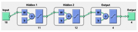
The optimal network architecture was selected after evaluating 25 MLP feedforward configurations. Considering multi-metric performance (MSE, RMSE, MAE, R, R²) and training efficiency, the final topology (18-11-12-4; Figure 1) comprised 18 input neurons (physical, granulometric, and mechanical parameters; Table 1), two hidden layers with 11 and 12 neurons, and 4 output neurons: Cement (C), Fine Aggregate (AF), Coarse Aggregate (AG), and Water (A).
Figure 1. Architecture of the optimized ANN model (18-11-12-4)
All layers employed the hyperbolic tangent sigmoid activation (tansig), as shown in Eq. (1). Its bounded [−1, 1] range ensured compatibility with normalized data, avoided saturation beyond the scaling range, and enabled smoother convergence during regression of continuous targets, providing advantages over ReLU in stability and learning efficiency for this dataset [15-17].
$f(x)=\frac{2}{1+e^{-2 x}}-1$ (1)
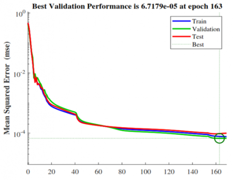
Figure 2. Training performance (MSE vs. epochs) and stopping at epoch 169
Compared to simpler architectures (e.g., 18-8-4 and 18-10-4), the 18-11-12-4 network (Figure 1) achieved lower errors and faster convergence, completing training in 4.577 seconds over 169 epochs (Figure 2), while avoiding overfitting.
2.2.2 Data preprocessing and normalization
Prior to training, data underwent two preprocessing steps:
(1). Outlier removal: A modified Z-score method was applied univariately to each of the 18 inputs and 4 outputs, using a threshold equivalent to a standard z-score > 3, to remove extreme values while preserving representative variability. Multivariate outlier detection was additionally performed using Mahalanobis distance.
(2). Normalization: All variables were scaled to the range [−1, 1] using MATLAB’s mapminmax function:
[X_norm, X_settings] = mapminmax(X, -1, 1);
[Y_norm, Y_settings] = mapminmax(Y, -1, 1);
(3). The [−1, 1] range was selected over [0, 1] because the tansig activation function outputs within this interval, enabling faster convergence, symmetric gradient propagation, and reduced bias shift during training.
New predictions were also automatically normalized and reversed:
Xnew_norm = mapminmax('apply', X_new, X_settings);
Ypred_norm = net(Xnew_norm);
Ypred = mapminmax('reverse', Ypred_norm, Y_settings);
Data were randomly split into mutually exclusive subsets:
•70% (564 samples) for training the model,
•15% (121 samples) for validation (early stopping and generalization assessment),
•15% (121 samples) for final testing of model performance.
All statistical analyses and modeling tasks were performed using MATLAB R2020a and RStudio 2024.12.0.
2.2.3 Training algorithm and parameters
The ANN was trained using the Levenberg-Marquardt (trainlm) backpropagation algorithm, ideal for small to medium-sized regression problems due to its fast convergence properties [18-20]. The learning process minimized the MSE between predicted and actual values using the following weight update rule:
$W_{\text {new }}=W_{\text {current }}-\left(J^T J+\mu I\right)^{-1} J^T E$ (2)
where, J: Jacobian matrix of partial derivatives, E: error vector, μ: damping parameter, I: identity matrix.
Training parameters included:
•Max. epochs: 1000,
•Performance goal: MSE < 0.001,
•Early stopping: Based on validation loss to avoid overfitting.
The final selected model converged in 169 epochs, reaching a minimum validation MSE of 6.7179×10⁻⁵, with training completed in 4.577 s.
2.2.4 Model evaluation and selection
Performance was assessed using MSE, RMSE, MAE, the correlation coefficient (R), and the coefficient of determination (R²). The selected network, saved as Mi_Red_23_30-Apr-2025_12-50-18, achieved the lowest prediction errors and the highest correlation among all candidates, with results summarized in Table 2.
Table 2. Selection of the RNA model with optimal number of neurons
|
Neural Network |
Configuration |
No. of Neurons |
Layers |
Time (s) |
Epochs |
MSE |
RMSE |
|
Mi_Red_2_04-Apr-2025_09-54-11 |
2 |
2 |
1 |
0.997 |
265 |
0.0403131 |
0.2007812 |
|
Mi_Red_3_04-Apr-2025_09-58-12 |
3 |
3 |
1 |
1.203 |
283 |
0.0123689 |
0.1112158 |
|
Mi_Red_4_04-Apr-2025_10-05-38 |
4 |
4 |
1 |
1.510 |
343 |
0.0030578 |
0.0552977 |
|
Mi_Red_5_04-Apr-2025_10-10-32 |
5 |
5 |
1 |
3.009 |
575 |
0.0010155 |
0.0318667 |
|
Mi_Red_6_04-Apr-2025_10-19-14 |
6 |
6 |
1 |
7.983 |
1000 |
0.0003107 |
0.0176256 |
|
Mi_Red_7_04-Apr-2025_10-36-55 |
7 |
7 |
1 |
4.456 |
491 |
0.0001571 |
0.0125331 |
|
Mi_Red_8_04-Apr-2025_10-42-47 |
8 |
8 |
1 |
4.366 |
437 |
0.0001342 |
0.0115865 |
|
Mi_Red_9_04-Apr-2025_10-53-42 |
9 |
9 |
1 |
1.869 |
182 |
0.0001825 |
0.0135090 |
|
Mi_Red_10_04-Apr-2025_11-10-12 |
10 |
10 |
1 |
6.021 |
496 |
0.0001163 |
0.0107854 |
|
Mi_Red_11_05-Apr-2025_18-21-26 |
11 |
11 |
1 |
4.465 |
335 |
0.0000967 |
0.0098344 |
|
Mi_Red_12_06-Apr-2025_21-06-02 |
12 |
12 |
1 |
9.297 |
548 |
0.0001001 |
0.0100050 |
|
Mi_Red_13_07-Apr-2025_15-50-34 |
13 |
13 |
1 |
2.661 |
175 |
0.0002341 |
0.0152994 |
|
Mi_Red_14_07-Apr-2025_17-08-16 |
5-9 |
14 |
2 |
1.377 |
135 |
0.0003616 |
0.0190161 |
|
Mi_Red_15_07-Apr-2025_19-42-51 |
15 |
15 |
1 |
0.873 |
46 |
0.0002623 |
0.0161951 |
|
Mi_Red_16_07-Apr-2025_22-18-31 |
16 |
16 |
1 |
5.965 |
280 |
0.0001059 |
0.0102927 |
|
Mi_Red_17_08-Apr-2025_22-40-24 |
11-6 |
17 |
2 |
1.366 |
86 |
0.0002042 |
0.0142885 |
|
Mi_Red_18_09-Apr-2025_15-35-39 |
9-9 |
18 |
2 |
1.718 |
107 |
0.0001406 |
0.0118593 |
|
Mi_Red_19_09-Apr-2025_19-16-44 |
8-11 |
19 |
2 |
2.952 |
192 |
0.0001366 |
0.0116881 |
|
Mi_Red_20_09-Apr-2025_21-18-17 |
20 |
20 |
1 |
2.920 |
95 |
0.0001964 |
0.0140128 |
|
Mi_Red_21_30-Apr-2025_05-52-10 |
10-11 |
21 |
2 |
3.669 |
120 |
0.0001225 |
0.0110674 |
|
Mi_Red_22_30-Apr-2025_12-13-28 |
11-11 |
22 |
2 |
4.455 |
135 |
0.0001120 |
0.0105809 |
|
Mi_Red_23_30-Apr-2025_12-50-18 |
11-12 |
23 |
2 |
4.577 |
169 |
0.0000790 |
0.0088878 |
|
Mi_Red_24_30-Apr-2025_16-28-26 |
12-12 |
24 |
2 |
5.478 |
223 |
0.0000886 |
0.0094144 |
|
Mi_Red_25_29-Apr-2025_22-25-05 |
25 |
25 |
1 |
4.76317 |
93 |
0.0002174 |
0.0147438 |
|
Mi_Red_26_30-Apr-2025_16-54-40 |
13-13 |
26 |
2 |
9.29952 |
295 |
0.0001574 |
0.0125477 |
|
Neural Network |
MAE |
R |
R² |
R_Train |
R_Val |
R_Test |
R_All |
|
Mi_Red_2_04-Apr-2025_09-54-11 |
0.1411534 |
0.9057636 |
0.8056782 |
0.9005815 |
0.9225107 |
0.9132399 |
0.9057636 |
|
Mi_Red_3_04-Apr-2025_09-58-12 |
0.0669657 |
0.9716091 |
0.9403778 |
0.9699969 |
0.9767442 |
0.9741472 |
0.9716091 |
|
Mi_Red_4_04-Apr-2025_10-05-38 |
0.0343151 |
0.9931767 |
0.9852603 |
0.9935817 |
0.9925506 |
0.9919635 |
0.9931767 |
|
Mi_Red_5_04-Apr-2025_10-10-32 |
0.0197422 |
0.9977045 |
0.9951050 |
0.9978015 |
0.9975035 |
0.9974901 |
0.9977045 |
|
Mi_Red_6_04-Apr-2025_10-19-14 |
0.0088247 |
0.9992988 |
0.9985025 |
0.9993334 |
0.9992414 |
0.9991804 |
0.9992988 |
|
Mi_Red_7_04-Apr-2025_10-36-55 |
0.0048894 |
0.9996445 |
0.9992428 |
0.9996857 |
0.9996013 |
0.9995004 |
0.9996445 |
|
Mi_Red_8_04-Apr-2025_10-42-47 |
0.0044917 |
0.9996967 |
0.9993529 |
0.9996826 |
0.9997900 |
0.9996695 |
0.9996967 |
|
Mi_Red_9_04-Apr-2025_10-53-42 |
0.0058671 |
0.9995870 |
0.9991203 |
0.9996217 |
0.9996659 |
0.9993383 |
0.9995870 |
|
Mi_Red_10_04-Apr-2025_11-10-12 |
0.0038229 |
0.9997365 |
0.9994393 |
0.9997988 |
0.9996702 |
0.9995125 |
0.9997365 |
|
Mi_Red_11_05-Apr-2025_18-21-26 |
0.0033469 |
0.9997807 |
0.9995338 |
0.9998178 |
0.9996800 |
0.9997043 |
0.9997807 |
|
Mi_Red_12_06-Apr-2025_21-06-02 |
0.0034740 |
0.9997733 |
0.9995175 |
0.9997928 |
0.9996812 |
0.9997753 |
0.9997733 |
|
Mi_Red_13_07-Apr-2025_15-50-34 |
0.0050154 |
0.9994702 |
0.9988717 |
0.9996609 |
0.9994423 |
0.9986847 |
0.9994702 |
|
Mi_Red_14_07-Apr-2025_17-08-16 |
0.0104667 |
0.9991824 |
0.9982569 |
0.9993331 |
0.9989912 |
0.9986538 |
0.9991824 |
|
Mi_Red_15_07-Apr-2025_19-42-51 |
0.0079158 |
0.9994134 |
0.9987357 |
0.9994486 |
0.9992448 |
0.9994271 |
0.9994134 |
|
Mi_Red_16_07-Apr-2025_22-18-31 |
0.0032436 |
0.9997598 |
0.9994893 |
0.9997782 |
0.9997456 |
0.9996817 |
0.9997598 |
|
Mi_Red_17_08-Apr-2025_22-40-24 |
0.0062812 |
0.9995404 |
0.9990159 |
0.9995366 |
0.9995996 |
0.9995034 |
0.9995404 |
|
Mi_Red_18_09-Apr-2025_15-35-39 |
0.0047115 |
0.9996824 |
0.9993221 |
0.9997333 |
0.9996383 |
0.9994792 |
0.9996824 |
|
Mi_Red_19_09-Apr-2025_19-16-44 |
0.0045869 |
0.9996907 |
0.9993415 |
0.9997218 |
0.9995517 |
0.9996811 |
0.9996907 |
|
Mi_Red_20_09-Apr-2025_21-18-17 |
0.0052839 |
0.9995547 |
0.9990535 |
0.9996573 |
0.9994404 |
0.9992002 |
0.9995547 |
|
Mi_Red_21_30-Apr-2025_05-52-10 |
0.0031081 |
0.9997226 |
0.9994096 |
0.9997918 |
0.9997799 |
0.9993803 |
0.9997226 |
|
Mi_Red_22_30-Apr-2025_12-13-28 |
0.0035718 |
0.9997464 |
0.9994603 |
0.9997739 |
0.9996152 |
0.9997520 |
0.9997464 |
|
Mi_Red_23_30-Apr-2025_12-50-18 |
0.0030581 |
0.9998210 |
0.9996192 |
0.9998215 |
0.9998393 |
0.9998035 |
0.9998210 |
|
Mi_Red_24_30-Apr-2025_16-28-26 |
0.0032353 |
0.9997993 |
0.9995728 |
0.9998162 |
0.9997897 |
0.9997303 |
0.9997993 |
|
Mi_Red_25_29-Apr-2025_22-25-05 |
0.0054465 |
0.9995081 |
0.9989522 |
0.999623 |
0.999042 |
0.9994180 |
0.9995080 |
|
Mi_Red_26_30-Apr-2025_16-54-40 |
0.0038596 |
0.9996500 |
0.9992411 |
0.999639 |
0.99968 |
0.9996740 |
0.9996500 |
Notes: The selection was based on a multi-metric evaluation framework. As summarized in Table 2, the chosen model achieved extremely low prediction errors, high correlation, and rapid convergence.
2.2.5 External validation with experimental mixes
The external validation of the artificial neural network (ANN) model Mi_Red_23_30-Apr-2025_12-50-18 was carried out using fifteen concrete mix designs that were not included in the training phase and were developed according to the ACI 221.1 procedure. These mixes were prepared with aggregates sourced from the La Moderna and Chillico quarries, with nominal compressive strengths of 140, 175, and 210 kg/cm². A total of 135 cylindrical specimens (6″×12″) were molded and cured following the guidelines of NTP 339.033:2021 and ASTM C31/C31M-2021. All specimens were stored in a curing chamber maintained at 20℃ ± 2℃ with a relative humidity above 95%, ensuring uniform curing conditions.
Table 3 provides a detailed description of the experimental datasets used in this validation stage. The data were subsequently processed by the neural network based on the previously learned weights, yielding predictions for the four main mixture components: cement, fine aggregate, coarse aggregate, and water. The validation procedure was implemented using the graphical interface of the NeuroMAT Toolbox v1.0, where the corresponding independent variables were entered. Finally, the model predictions are presented in Table 4, demonstrating the ANN’s predictive capacity when applied to experimental mixtures independent from the training dataset.
Table 3. Experimental data for the validation of the RNA model
|
Origin |
Mix ID |
f′c Design (kg/cm²) |
Real |
|||
|
Cement (kg/m³) |
Fine Agg. (kg/m³) |
Coarse Agg. (kg/m³) |
Water (l/m³) |
|||
|
La Moderna |
MM1 |
140 |
299.708 |
897.444 |
848.030 |
206.092 |
|
175 |
326.433 |
875.151 |
848.030 |
206.266 |
||
|
210 |
367.120 |
841.212 |
848.030 |
206.530 |
||
|
MM2 |
140 |
299.708 |
889.552 |
880.604 |
202.169 |
|
|
175 |
326.433 |
867.147 |
880.604 |
202.487 |
||
|
210 |
367.120 |
833.037 |
880.604 |
202.971 |
||
|
MM3 |
140 |
299.708 |
890.326 |
848.302 |
216.663 |
|
|
175 |
326.433 |
868.403 |
848.302 |
216.660 |
||
|
210 |
367.120 |
835.028 |
848.302 |
216.657 |
||
|
Chillico |
CM1 |
140 |
315.789 |
937.104 |
704.650 |
243.416 |
|
175 |
343.949 |
914.895 |
704.650 |
243.042 |
||
|
210 |
386.819 |
881.085 |
704.650 |
242.472 |
||
|
CM2 |
140 |
315.789 |
1007.228 |
668.061 |
233.392 |
|
|
175 |
343.949 |
984.458 |
668.061 |
233.199 |
||
|
210 |
386.819 |
949.792 |
668.061 |
232.905 |
||
Table 4. Mixture dosages predicted by the RNA model
|
Origin |
Mix ID |
f′c Design (kg/cm²) |
ANN |
|||
|
Cement (kg/m³) |
Fine Agg. (kg/m³) |
Coarse Agg. (kg/m³) |
Water (l/m³) |
|||
|
La Moderna |
MM1 |
140 |
297.798 |
888.337 |
864.137 |
207.701 |
|
175 |
323.153 |
866.991 |
865.078 |
207.656 |
||
|
210 |
364.680 |
835.383 |
866.994 |
207.625 |
||
|
MM2 |
140 |
299.109 |
873.601 |
883.039 |
202.990 |
|
|
175 |
327.562 |
854.552 |
881.121 |
203.240 |
||
|
210 |
369.580 |
818.376 |
879.184 |
203.310 |
||
|
MM3 |
140 |
298.387 |
885.999 |
852.950 |
217.512 |
|
|
175 |
323.527 |
862.334 |
855.073 |
216.920 |
||
|
210 |
363.301 |
826.224 |
856.347 |
216.995 |
||
|
Chillico |
CM1 |
140 |
319.874 |
937.484 |
730.811 |
243.821 |
|
175 |
350.470 |
912.830 |
732.990 |
243.497 |
||
|
210 |
393.537 |
875.978 |
732.169 |
243.213 |
||
|
CM2 |
140 |
311.638 |
1003.826 |
666.547 |
233.763 |
|
|
175 |
338.243 |
974.313 |
666.582 |
233.498 |
||
|
210 |
381.394 |
932.745 |
666.601 |
233.305 |
||
Table 5. Percentage Error (PE) and Mean Squared Error (MSE) for ANN predictions compared to experimental dosages
|
Origin |
Mix ID |
f′c Design (kg/cm²) |
Percentage Error (PE) (%) |
|||
|
Cement PE (%) |
Fine Agg. PE (%) |
Coarse Agg. PE (%) |
Water PE (%) |
|||
|
La Moderna |
MM1 |
140 |
0.64 |
1.01 |
1.90 |
0.78 |
|
175 |
1.00 |
0.93 |
2.01 |
0.67 |
||
|
210 |
0.66 |
0.69 |
2.24 |
0.53 |
||
|
MM2 |
140 |
0.20 |
1.79 |
0.28 |
0.41 |
|
|
175 |
0.35 |
1.45 |
0.06 |
0.37 |
||
|
210 |
0.67 |
1.76 |
0.16 |
0.17 |
||
|
MM3 |
140 |
0.44 |
0.49 |
0.55 |
0.39 |
|
|
175 |
0.89 |
0.70 |
0.80 |
0.12 |
||
|
210 |
1.04 |
1.05 |
0.95 |
0.16 |
||
|
Chillico |
CM1 |
140 |
1.29 |
0.04 |
3.71 |
0.17 |
|
175 |
1.90 |
0.23 |
4.02 |
0.19 |
||
|
210 |
1.74 |
0.58 |
3.91 |
0.31 |
||
|
CM2 |
140 |
1.31 |
0.34 |
0.23 |
0.16 |
|
|
175 |
1.66 |
1.03 |
0.22 |
0.13 |
||
|
210 |
1.40 |
1.79 |
0.22 |
0.17 |
||
|
MAPE (%) |
1.01 |
0.93 |
1.42 |
0.31 |
||
|
MSE |
15.76 |
92.01 |
220.10 |
0.62 |
||
|
Max PE (%) |
4.02 |
|||||
Table 5 shows that the ANN model achieves a high level of accuracy, with both absolute and percentage errors generally low. The coarse aggregate registers the highest percentage error (4.02%), while the overall average error across all components remains below 1.5%. The higher deviation observed for coarse aggregate can be attributed to the intrinsic variability in particle packing and gradation within the experimental dataset, as well as the underrepresentation of certain high-strength mixes in which coarse aggregate proportions deviate more markedly from the mean. Regarding the MSE, the largest value also corresponds to coarse aggregate (220.10), followed by fine aggregate (92.01), although both remain within acceptable tolerance limits, confirming the model’s robustness despite these localized variations.
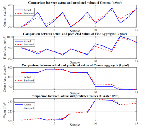
Figure 3 compares the experimental values (ACI 211.1) with those estimated by the ANN for cement, fine aggregate, coarse aggregate, and water. The blue line represents the experimental data, while the red dashed line corresponds to the model predictions. An adequate fit is observed between both curves, particularly for cement and water, with minor discrepancies in fine and coarse aggregates. These results confirm the accuracy and predictive capability of the ANN in the efficient design of concrete mixes.
Figure 3. Experimental vs. predicted concrete mix components (ANN)
2.3 MLRM
2.3.1 Model specification and estimation
To benchmark the predictive capacity of the ANN, an MLRM was implemented using the same 18 input variables and 4 output variables. This method captures linear dependencies between predictors and dosage components. Recent studies have successfully applied similar models in concrete mix design and property prediction [21-23].
The multivariate regression model is formally expressed in matrix notation as:
$Y=X \cdot B+E$ (3)
where,
Y $\in$ ℝⁿˣ⁴: Matrix of dependent variables (dosage outputs: C, AF, AG, A)
X $\in$ ℝn×19: Matrix of independent variables, including an intercept and 18 predictors
B $\in$ ℝ19×4: Matrix of regression coefficients
E $\in$ ℝn×4: Matrix of residual errors
The coefficient matrix B was estimated using the Ordinary Least Squares (OLS) method:
$\widehat{B}=\left(X^T \cdot X\right)^{-1} \cdot X^T \cdot Y$ (4)
This estimation minimizes the sum of squared residuals and provides the best linear unbiased estimators (BLUE), assuming the classical regression assumptions hold (linearity, homoscedasticity, independence, and normality of residuals).
(1) Implementation in R
The MLRM was implemented in RStudio 2024.12.0 using the built-in lm() function and the command summary(modelo) was used with the following structure:
modelo <- lm(cbind(y1, y2, y3, y4) ~ x1 + x2 + ... + x18, data = datos)
summary(modelo)
where, y1 to y4 denote the four output variables (C, AF, AG, A), and x1 to x18 represent the 18 input predictors.
(2) Regression equations
The resulting system produced four independent regression equations of the form:
$\hat{y}_k=\beta_{0 k}+\sum_{j=1}^{18} \beta_{j k} x_j+\varepsilon_k$ (5)
where,
$\hat{y}_k$: Predicted value of output variable k
$\beta_{0 k}$: Intercept for equation k
$\beta_{j k}$: Coefficient for predictor xjin equation k
$\varepsilon_k$: Random error term associated with output k
Each equation captures the additive linear influence of the 18 input features on a specific output variable.
2.3.2 Statistical evaluation of fit
Residual diagnostics, statistical significance (p-values), and performance metrics were computed for each dependent variable. The complete data matrix included 806 samples with full multivariate observations.
(1) Goodness-of-fit metrics
All R² values were statistically significant (p < 0.001), indicating strong model performance, particularly for water and coarse aggregate prediction, as summarized in Table 6.
Table 6. Goodness-of-fit metrics for each dependent variable in the MLRM
|
Output Variable |
R² |
Adj. R² |
RMSE |
MSE |
|
Cement (y₁) |
0.8418 |
0.8382 |
18.34 |
336.25 |
|
Fine Aggregate (y₂) |
0.9069 |
0.9047 |
23.54 |
554.34 |
|
Coarse Aggregate (y₃) |
0.9710 |
0.9703 |
14.38 |
206.81 |
|
Water (y₄) |
0.9968 |
0.9967 |
1.59 |
2.52 |
(2) Model significance: ANOVA and MANOVA tests
Two complementary statistical tests were applied:
•Univariate ANOVA assessed each dependent variable individually, confirming that the predictors significantly influenced all four outputs (p < 0.001) [24].
•Multivariate MANOVA evaluated the predictors’ joint effect across all dependent variables, using Wilks’ Lambda, Pillai’s Trace, Hotelling-Lawley, and Roy’s Root, all of which confirmed strong multivariate significance (p < 0.001) as shown in Table 7 [25, 26].
Table 7. MANOVA statistics summary
|
Test |
Statistic |
p-value |
Interpretation |
|
Wilks’ Lambda (Λ) |
≈ 0 |
< 0.001 |
Strong multivariate effect |
|
Pillai's Trace (V) |
≈ 1 |
< 0.001 |
Robust multivariate significance |
|
Hotelling-Lawley (U) |
High |
< 0.001 |
Large proportion of variance explained |
|
Roy’s Root (θ) |
High |
< 0.001 |
Key variables (x₄, x₇, x₁₃, x₁₇) dominate the model |
Table 8. Computational demand comparison (MLRM vs. ANN)
|
Model |
Runtime |
Complexity |
|
MLRM |
< 1 s |
Low (direct OLS) |
|
ANN |
1-10 s |
High (iterative training over ~46-1000 epochs) |
The rationale for using MANOVA alongside ANOVA is that while ANOVA detects effects in each response variable independently, MANOVA accounts for correlations among responses, providing a more comprehensive assessment when dependent variables are related (as in concrete mix proportions) [24-26].
(3) Collinearity diagnostics
Variance Inflation Factor (VIF) analysis was conducted to assess multicollinearity among predictors. All VIF values were below the commonly accepted threshold of 5, indicating that collinearity was not a concern and that coefficient estimates are stable.
(4) Computational demand
Computational efficiency was compared between the MLRM and the ANN. As shown in Table 8, the MLRM computed solutions in less than one second via direct Ordinary Least Squares (OLS), while the ANN required 1–10 seconds due to iterative weight optimization over approximately 46–1000 epochs. This highlights a trade-off: the MLRM offers speed and simplicity for linear relations, whereas the ANN provides greater flexibility and non-linear mapping capabilities, albeit with higher computational cost.
2.3.3 Assumption diagnostics
Model assumptions were evaluated as follows (see Figures 4–6):
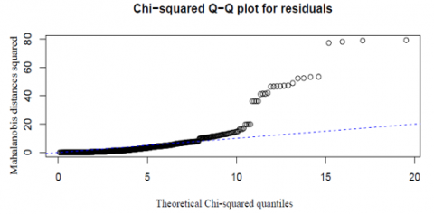
•Normality: Mahalanobis Q-Q plots (Figure 4) confirmed approximate multivariate normality.
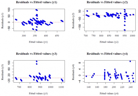
•Homoscedasticity: Residual vs. fitted plots (Figure 5) showed no significant patterns, indicating constant variance.
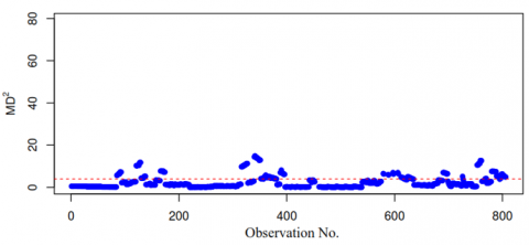
•Independence: Serial correlation plots of MD² values (Figure 6) showed no significant autocorrelation.
Figure 4. Chi-square Q-Q plot for multivariate residuals
Figure 5. Residuals vs. fitted values plot
Figure 6. Serial correlation plot of MD²
Following the validation protocol applied to the ANN model, a similar evaluation was performed for the MLRM. Table 9 presents the predicted mix proportions for 15 concrete mix designs obtained with the MLRM model. Table 10 summarizes the absolute (AE) and percentage errors between measured and predicted values. The average percentage errors for cement, fine aggregate, coarse aggregate, and water were 2.62%, 1.21%, 0.96%, and 0.87%, respectively, with a maximum PE of 6.24% observed in cement dosage.
Table 9. Predicted mix proportions using the MLRM model
|
Origin |
Mix ID |
f′c Design (kg/cm²) |
MLRM |
|||
|
Cement (kg/m³) |
Fine Agg. (kg/m³) |
Coarse Agg. (kg/m³) |
Water (l/m³) |
|||
|
La Moderna |
MM1 |
140 |
296.237 |
902.372 |
847.958 |
202.096 |
|
175 |
320.053 |
882.616 |
843.373 |
203.415 |
||
|
210 |
347.345 |
858.967 |
841.461 |
204.848 |
||
|
MM2 |
140 |
309.156 |
885.479 |
882.843 |
202.420 |
|
|
175 |
335.426 |
862.983 |
880.146 |
203.814 |
||
|
210 |
359.443 |
842.993 |
875.715 |
205.147 |
||
|
MM3 |
140 |
300.157 |
885.021 |
849.347 |
216.404 |
|
|
175 |
326.834 |
862.069 |
846.962 |
217.810 |
||
|
210 |
350.213 |
842.792 |
842.041 |
219.124 |
||
|
Chillico |
CM1 |
140 |
322.025 |
912.891 |
725.596 |
243.599 |
|
175 |
350.880 |
887.507 |
724.886 |
245.071 |
||
|
210 |
376.885 |
865.295 |
721.984 |
246.466 |
||
|
CM2 |
140 |
335.496 |
992.856 |
679.344 |
233.932 |
|
|
175 |
358.123 |
974.430 |
673.845 |
235.214 |
||
|
210 |
382.928 |
953.560 |
670.020 |
236.572 |
||
Table 10. PE and MSE for MLRM predictions compared to experimental dosages
|
Origin |
Mix ID |
f′c Design (kg/cm²) |
PE (%) |
|||
|
Cement PE (%) |
Fine Agg. PE (%) |
Coarse Agg. PE (%) |
Water PE (%) |
|||
|
La Moderna |
MM1 |
140 |
1.16 |
0.55 |
0.01 |
1.94 |
|
175 |
1.95 |
0.85 |
0.55 |
1.38 |
||
|
210 |
5.39 |
2.11 |
0.77 |
0.81 |
||
|
MM2 |
140 |
3.15 |
0.46 |
0.25 |
0.12 |
|
|
175 |
2.75 |
0.48 |
0.05 |
0.66 |
||
|
210 |
2.09 |
1.20 |
0.56 |
1.07 |
||
|
MM3 |
140 |
0.15 |
0.60 |
0.12 |
0.12 |
|
|
175 |
0.12 |
0.73 |
0.16 |
0.53 |
||
|
210 |
4.61 |
0.93 |
0.74 |
1.14 |
||
|
Chillico |
CM1 |
140 |
1.97 |
2.58 |
2.97 |
0.08 |
|
175 |
2.02 |
2.99 |
2.87 |
0.83 |
||
|
210 |
2.57 |
1.79 |
2.46 |
1.65 |
||
|
CM2 |
140 |
6.24 |
1.43 |
1.69 |
0.23 |
|
|
175 |
4.12 |
1.02 |
0.87 |
0.86 |
||
|
210 |
1.01 |
0.40 |
0.29 |
1.57 |
||
|
MAPE (%) |
2.62 |
1.21 |
0.96 |
0.87 |
||
|
MSE |
116.61 |
170.92 |
96.63 |
5.26 |
||
|
Max PE (%) |
6.24 |
|||||
Finally, Figure 7 shows the comparison between the actual experimental values (ACI 211.1) and those predicted by the RLMM model for the variables: cement, fine aggregate, coarse aggregate, and water. The blue lines represent the experimental data, while the dashed red lines represent the predictions. Overall, good agreement is observed, with a close fit for coarse aggregate and water. Cement and fine aggregate exhibit some variations but maintain the overall trend, demonstrating the model’s effectiveness.
Figure 7. Experimental vs. predicted concrete mix components (C, AF, AG, A) by the MLRM model
3.1 Performance of the ANN model
The predictive performance of the ANN and the MLRM was evaluated using the same experimental dataset. To enable a clearer comparison, the results are presented in Table 11, which summarizes the performance metrics for each target variable: cement, fine aggregate, coarse aggregate, and water. The ANN, implemented as a MLP with an 18-11-12-4 topology and trained via the Levenberg-Marquardt algorithm, demonstrated excellent predictive capability across all variables. This architecture was selected after iterative testing for its balance between complexity and computational efficiency, effectively capturing nonlinear interactions.
By contrast, the MLRM, although capable of modeling general trends, showed reduced predictive accuracy for cement and fine aggregate due to its inability to account for such nonlinearities. Interestingly, for coarse aggregate, the MLRM performed slightly better in RMSE and MAE, likely because this variable presents a more linear relationship with other mix parameters.
Table 11. Performance metrics for ANN and MLRM models by output variable
|
Variable |
RMSE (ANN) |
RMSE (MLRM) |
MAE (ANN) |
MAE (MLRM) |
MSE (ANN) |
MSE (MLRM) |
MAPE% (ANN) |
|
Cement |
3.970 |
10.799 |
3.498 |
8.958 |
15.759 |
116.610 |
1.013 |
|
Fine Aggregate |
9.592 |
13.074 |
8.243 |
10.887 |
92.011 |
170.924 |
0.926 |
|
Coarse Aggregate |
14.836 |
9.830 |
10.829 |
7.005 |
220.103 |
96.627 |
1.416 |
|
Water |
0.787 |
2.293 |
0.675 |
1.906 |
0.619 |
5.257 |
0.314 |
|
Variable |
MAPE% (MLRM) |
R (ANN) |
R (MLRM) |
R² (ANN) |
R² (MLRM) |
NSE (ANN) |
NSE (MLRM) |
|
Cement |
2.620 |
0.992 |
0.935 |
0.984 |
0.874 |
0.982 |
0.867 |
|
Fine Aggregate |
1.208 |
0.996 |
0.973 |
0.991 |
0.947 |
0.964 |
0.933 |
|
Coarse Aggregate |
0.958 |
0.992 |
0.997 |
0.984 |
0.994 |
0.970 |
0.987 |
|
Water |
0.867 |
0.999 |
0.994 |
0.998 |
0.988 |
0.997 |
0.978 |
3.2 Global performance summary
3.2.1 Variable-level evaluation
Table 12 shows the ANN demonstrates superior performance to the MLRM across all evaluation metrics, with particularly strong improvements in error reduction (18.9-35.1%) while maintaining excellent correlation and efficiency scores (all above 0.97). The most significant improvement is seen in MAPE (35.1% better), indicating the ANN's particular strength at minimizing percentage errors.
Table 12. Global average performance metrics for ANN and MLRM
|
Metric |
ANN |
MLRM |
ANN Improvement |
|
RMSE (kg/m³) |
7.296 |
8.999 |
18.9% |
|
MAE (kg/m³) |
5.811 |
7.189 |
19.2% |
|
MSE (kg²/m⁶) |
82.123 |
97.355 |
15.6% |
|
MAPE (%) |
0.918 |
1.413 |
35.1% |
|
Correlation (R) |
0.9947 |
0.9747 |
2.1% |
|
Determination (R²) |
0.9895 |
0.9507 |
4.1% |
|
Nash-Sutcliffe (NSE) |
0.9784 |
0.9413 |
3.9% |
3.3 Trends and visual validation
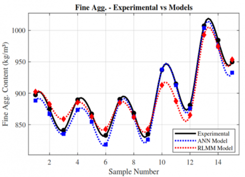
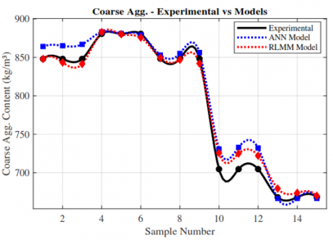
Visual comparison between predicted and experimental values (Figures 8-11) confirmed that both models reproduced the general experimental trends. However, the ANN consistently exhibited higher precision, particularly for cement and water content, where the MLRM showed greater dispersion. The only variable where MLRM slightly outperformed ANN was coarse aggregate likely due to its more linear dependence on volumetric constraints.
Figure 8. Comparison between predicted and experimental cement content using ANN and MLRM models
Figure 9. Comparison between predicted and experimental fine aggregate content using ANN and MLRM models
Figure 10. Comparison between predicted and experimental coarse aggregate content using ANN and MLRM models
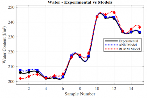
Figure 11. Comparison between predicted and experimental water content using ANN and MLRM models
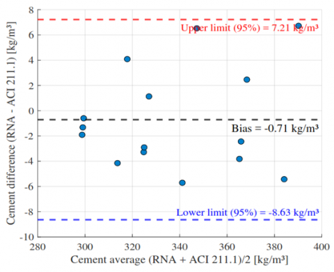
3.4 Bland-Altman agreement analysis
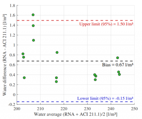
To complement the correlation and error-based performance metrics, a Bland-Altman analysis was conducted to evaluate the agreement between the ANN predictions and the conventional ACI 211.1 method for each output variable (Figures 12-15). This approach quantifies the systematic bias (mean difference) and the 95% limits of agreement, offering a more robust assessment of predictive consistency than correlation alone [27, 28].
Figure 12. Bland-Altman plot for cement content: ANN vs. ACI 211.1
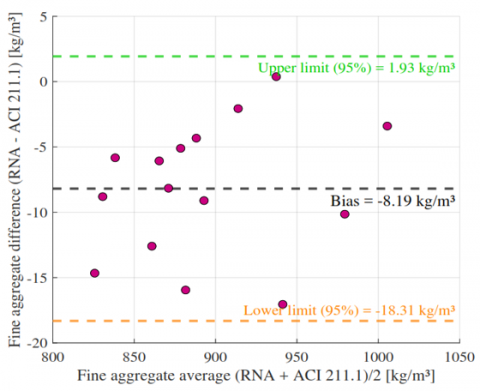
Figure 13. Bland-Altman plot for fine aggregate content: ANN vs. ACI 211.1
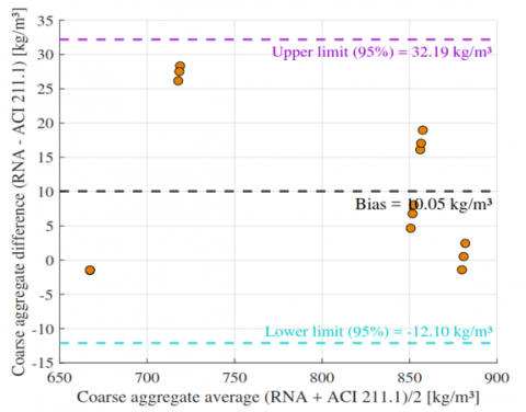
For cement (Figure 12), the ANN showed a negligible bias of −0.71 kg/m³ with limits of agreement from −8.63 to +7.21 kg/m³, indicating strong agreement and no proportional bias. Fine aggregate (Figure 13) presented a slightly larger underestimation (−8.19 kg/m³) but remained within acceptable limits (−18.31 to +1.93 kg/m³). Coarse aggregate (Figure 14) exhibited a tendency toward overestimation (+10.05 kg/m³) and higher variability (limits: −12.10 to +32.19 kg/m³), suggesting an opportunity for further refinement. In contrast, water content (Figure 15) demonstrated excellent agreement, with a minimal bias of +0.67 l/m³ and narrow limits (−0.15 to +1.50 l/m³).
Figure 14. Bland-Altman plot for coarse aggregate content: ANN vs. ACI 211.1
Figure 15. Bland-Altman plot for water content: ANN vs. ACI 211.1
Overall, the Bland-Altman plots confirm that the ANN achieves high concordance with ACI 211.1, particularly for cement and water the most critical parameters in mix design while fine aggregate performance remains acceptable and coarse aggregate results highlight an area for targeted improvement.
3.5 Sustainability impact
The ANN-based mix design yielded an average cement reduction of 10.644 kg/m³ compared to ACI 211.1 without compromising strength predictions. Assuming an emission factor of 0.90 tCO₂/t cementa standard value reported in the literature for clinker-based Portland cement production this reduction translates into ≈9.58 tCO₂ saved per 1000 m³ of concrete.
This study confirms that ANNs, particularly a multilayer perceptron with an 18-11-12-4 architecture, are a robust and efficient solution for optimizing concrete mix design under the unique high-altitude conditions of Ayacucho, Peru. By incorporating local aggregate mineralogy and site-specific environmental factors, the ANN achieved R² = 0.9895, NSE = 0.9784, and a global MAPE = 0.9175%, outperforming MLRM in all metrics (R² = 0.9507, NSE = 0.9413, MAPE = 1.4130%). Bland-Altman analysis further validated its strong agreement with the ACI 211.1 method for critical mix variables.
From a sustainability standpoint, the ANN-based approach reduced cement overuse by 3.0%, generating an average cost saving of USD 2.12 per cubic meter and lowering waste and CO₂ emissions. These results demonstrate the model’s potential to deliver both economic and environmental benefits in regions with similar geological and climatic characteristics.
Future work should include: (1) calibrating the model for diverse aggregate sources considering mineralogical and absorption variability; (2) integrating mobile design applications and real-time sensor data feeds; (3) incorporating advanced algorithms—Random Forest, Gradient Boosting, XGBoost, LightGBM, and Support Vector Machines—to evolve from predictive to prescriptive mix design, optimizing for strength, cost, and sustainability; and (4) expanding scope to durability parameters such as chloride penetration resistance and freeze-thaw performance to ensure long-term structural reliability.
The authors wish to express their gratitude to the Faculty of Mining, Geology, and Civil Engineering at the Universidad Nacional de San Cristóbal de Huamanga for the institutional support provided during the development of this research.
[1] Oh, J.W., Lee, I.W., Kim, J.T. (1999). Application of neural networks for proportioning of concrete mixes. ACI Structural Journal, 96(1): 61-67. https://doi.org/10.14359/429
[2] Setién, J., Carrascal, I.A., Figueroa, J.F., Polanco, J.A. (2025). Application of an artificial neural network to ready-mixed concretes mix design. Materiales de Construcción, 53(270): 5-20. https://doi.org/10.3989/MC.2003.V53.I270.270
[3] Yousif, S.T., Algburi, M.A., Abdulkareem, O.M. (2010). Design of concrete mixes using artificial neural networks. https://www.researchgate.net/publication/236945405_DESIGN_OF_CONCRETE_MIXES_USING_ARTIFICIAL_NEURAL_NETWORKS.
[4] Gowda, K., Prasad, G.L.E. (2011). Prognostication of concrete mix proportion by an approach. Advanced Materials Research, 261-263: 426-430. https://doi.org/10.4028/www.scientific.net/AMR.261-263.426
[5] Hasan, M.M. (2012). Artificial neural network for concrete mix design. Ukieri Concrete Congress-Innovations in Concrete Construction. https://www.researchgate.net/publication/275520307_Artificial_Neural_Network_for_Concrete_Mix_Design.
[6] Sachan, A.K., Ramashankar. (2014). Concrete mix design using neural network. https://www.academia.edu/116783045/Concrete_Mix_Design_Using_Neural_Network.
[7] Das, S. Pal, P., Singh, R.M. (2015). Prediction of concrete mix proportion using ANN technique. International Research Journal of Engineering and Technology, 2(5): 820-825. https://www.irjet.net/archives/V2/i5/IRJET-V2I5140.pdf.
[8] Rahmani, H., Ahmadi, S., Mansorkhani, A.A. (2018). Reliable neural networks for proportioning of concrete mixes containing cement replacement materials. Advances in Civil Engineering Materials, 7(1): 633-650. https://doi.org/10.1520/ACEM20180023
[9] Açikgenç, M., Ulaş, M., Alyamaç, K.E. (2015). Using an artificial neural network to predict mix compositions of steel fiber-reinforced concrete. Arabian Journal for Science & Engineering, 40: 407-419. https://doi.org/10.1007/s13369-014-1549-x
[10] Huang, Y., Zhang, J., Ann, F.T., Ma, G. (2020). Intelligent mixture design of steel fibre reinforced concrete using a support vector regression and firefly algorithm based multi-objective optimization model. Construction and Building Materials, 249: 120457. https://doi.org/10.1016/j.conbuildmat.2020.120457
[11] Jagadesh, P., Annamalai, A., Srivastava, A., Elango, K., et al. (2024). Artificial neural network, machine learning modelling of compressive strength of recycled coarse aggregate based self-compacting concrete. PLoS One, 19(5): e0303101. https://doi.org/10.1371/journal.pone.0303101
[12] Adil, M. Ullah, R. Noor, S. Gohar, N. (2022). Effect of number of neurons and layers in an artificial neural network for generalized concrete mix design. Neural Computing and Applications, 34(11): 8355-8363. https://doi.org/10.1007/s00521-020-05305-8
[13] Zheng, W., Shui, Z., Xu, Z., Gao, X., et al. (2023). Multi-objective optimization of concrete mix design based on machine learning. Journal of Building Engineering, 76: 107396. https://doi.org/10.1016/j.jobe.2023.107396
[14] Arbazoddin, S. Patki, V.K. Kulkarni, G., Jahagirdar, S., et al. (2024). Artificial neural network for concrete mix design. International Journal of Intelligent Systems and Applications in Engineering, 12(21): 3186-3198.
[15] Liu, X., Di, X. (2021). Tanhexp: A smooth activation function with high convergence speed for lightweight neural networks. IET Computer Vision, 15(2): 136-150. https://doi.org/10.1049/cvi2.12020
[16] Dubey, S.R., Singh, S.K., Chaudhuri, B.B. (2021). Activation functions in deep learning: A comprehensive survey and benchmark. arXiv preprint arXiv:2109.14545. https://arxiv.org/abs/2109.14545
[17] Mastromichalakis, S. (2023). Parametric leaky tanh: A new hybrid activation function for deep learning. arXiv preprint arXiv:2310.07720. https://arxiv.org/abs/2310.07720
[18] Yan, Z., Zhong, S., Lin, L., Cui, Z. (2021). Adaptive Levenberg-Marquardt algorithm: A new optimization strategy for Levenberg-Marquardt neural networks. Mathematics, 9(17): 2176. https://doi.org/10.3390/math9172176
[19] Martínez, J.M. (2024). Levenberg-Marquardt revisited and parameter tuning of river regression models. Computational & Applied Mathematics, 43(1). https://doi.org/10.1007/s40314-023-02535-z
[20] Bilski, J., Smolg, J., Kowalczyk, B., Grzanek, K., et al. (2023). Fast computational approach to the Levenberg-Marquardt algorithm for training feedforward neural networks. Journal of Artificial Intelligence and Soft Computing Research, 13(2): 45-61. https://doi.org/10.2478/jaiscr-2023-0006
[21] Zheng, W., Shui, Z., Xu, Z., Gao, X., Zhang, S. (2023). Multi-objective optimization of concrete mix design based on machine learning. Journal of Building Engineering, 76: 107396. https://doi.org/10.1016/j.jobe.2023.107396
[22] Imran, H., Al-Abdaly, N.M., Shamsa, M.H., Shatnawi, A., et al. (2022). Development of prediction model to predict the compressive strength of eco-friendly concrete using multivariate polynomial regression combined with stepwise method. Materials, 15(1): 317. https://doi.org/10.3390/ma15010317
[23] Harith, I.K., Nadir, W., Salah, M.S.H.M.L. (2024). Prediction of high-performance concrete strength using machine learning with hierarchical regression. Multiscale and Multidisciplinary Modeling, Experiments and Design, 7(5): 4911-4922. https://doi.org/10.1007/s41939-024-00467-7
[24] Xie, H.S., Gandla, S.R., Shi, O., Solanki, P. (2023). Multivariate regression and variance in concrete curing methods: Strength prediction with experiments. Applied Sciences-Basel, 13(22): 21. https://doi.org/10.3390/app132212239
[25] Montelongo, A., Pacheco, F., Christ, R., Tutikian, B.F. (2020). Study on concrete through its hardened state properties. Revista IBRACON de Estruturas e Materiais, 13(1): 87-94. https://doi.org/10.1590/S1983-41952020000100007
[26] Shenoy, A., Nayak, G., Tantri, A., Shetty, K.K., et al. (2023). Annual transmittance behavior of light-transmitting concrete with optical fiber bundles. Materials, 16(21): 7037. https://doi.org/10.3390/ma16217037
[27] Doğan, N.Ö. (2018). Bland-Altman analysis: A paradigm to understand correlation and agreement. Turkish Journal of Emergency Medicine, 18(4): 139-141. https://doi.org/10.1016/j.tjem.2018.09.001
[28] Bland, J.M., Altman, D. (1986). Statistical methods for assessing agreement between two methods of clinical measurement. Lancet, 327(8476): 307-310. https://doi.org/10.1016/S0140-6736(86)90837-8