Marwan S. Jameel*![]() | Ali A. Al-Arbo
| Ali A. Al-Arbo![]() | Rana Z. Al-Kawaz
| Rana Z. Al-Kawaz![]()
© 2025 The authors. This article is published by IIETA and is licensed under the CC BY 4.0 license (http://creativecommons.org/licenses/by/4.0/).
OPEN ACCESS
Conjugate gradient techniques are iterative algorithms used to solve unconstrained optimization problems. Hybrid techniques, which employ the conjugate gradient technique, are a branch of these algorithms. We apply the maximum mathematical function to group the essential quantities and determine the associated new conjugate gradient (CG) parameter that produces homogeneous and mixed and spectral gradient algorithms. The newly created parameter has a numerator containing the most important values from the investigation and a denominator with the most important quantities. Furthermore, using precise inspection operations, the conjugate hybrid gradient technique meets global convergence requirements. Numerical tests on a variety of test functions show that the proposed method has better convergence properties and is more efficient at computing. The parameters $\beta_k^N$ and $\theta_k^N$ determine the new direction. These algorithms can yield favourable ratios in particular scenarios, which is an advantage. Globally convergent functions are defined as convex functions that exhibit uniform genericity. We have shown numerical data that compare our newly proposed CG algorithms with standard algorithms to illustrate the efficacy of our approach. The results were obtained using the parameters $\beta_k^N$ and $\theta_k^N$.
general conjugate gradient (GCG) method, analysis global convergence, spectral conjugate gradient (SCG), Wolfe line process (WC), numerical tests
Consider these unconstrained optimization problems [1]:
$\min f(x), \quad x \in R^n$ (1)
The function $f$ is a mapping from the $n$ dimensional real numbers to the real numbers. The gradient of function $f$ at point $x$ is a continuous and differentiable function that represents the set of real numbers $R$. In the subject of mathematics, there are three main groups of solutions: exact, approximate, and numerical approaches. Several numerical techniques can be employed to solve Eq. (1), including the Newton method, the conjugate gradient method, the steepest descent method, and the quasi-Newton method. The conjugate gradient method is indispensable, especially for problems of significant magnitude, owing to its straightforwardness and little memory use. The conjugate gradient approach is extremely efficient. The numerical type was categorized using conjugate gradient techniques, alternatively, one of its enhancements. The bracketing method entails commencing with an initial estimate $x^0$ and subsequently iteratively approaching a solution for Eq. (1) by decreasing until we reach an iteration $x^n$. At this juncture, we initially calculate the objective function $f(x)$ and proceed to calculate it for following iterations $x^1, x^2, x^3, x^4, x^5, \ldots$ and so on based on Eq. (2). The development of a non-linear conjugate gradient method often entails an iterative procedure with the goal of attaining the optimal solution [2].
$x_{k+1}=x_k+\lambda_k p_k$ (2)
$\lambda_k$ the step-length is typically determined by doing a sequence of line searches proses. The step length $x^k$ can be chosen using the Wolfe, Goldstein, or Armijo criterion to provide a sufficient reduction in the function value without too short steps. The direction $p^k$ is established when two terms are present [3].
$p_{k+1}= \begin{cases}-g_{k+1} & \text { if } k=0, \\ -g_{k+1}+\beta_k p_k & \text { if } k>0,\end{cases}$ (3)
Further, for the three-term conjugate gradient (TTCG), Andrei [4] stated that technique enables the use of generic forms.
$p_{k+1}=\left\{\begin{array}{lr}-g_{k+1} & \text { if } k=0, \\ -g_{k+1}+a s_k-b v_k & \text { if } k>0,\end{array}\right.$ (4)
Methods yield distinct formulas both in practical and analytical contexts are based on the selection of the conjugate parameter. The most renowned among them are:
Table 1. Conjugacy parameters for slandered conjugate gradients
|
$\beta_k^{F R}=\frac{g_{k+1}^T g_{k+1}}{g_k^T g_k}$ [5] |
$\beta_k^{C D}=\frac{g_{k+1}^T g_{k+1}}{-p_k^T g_k}$ [6] |
$\beta_k^{B A 1}=\frac{y_k^T y_k}{-p_k^T g_k}$ [7] |
|
$\beta_k^{H S}=\frac{g_{k+1}^T y_k}{d_k^T y_k}$ [8] |
$\beta_k^{L S}=\frac{g_{k+1}^T g_k}{-p_k^T g_k}$ [9] |
$\beta_k^{B A 2}=\frac{y_k^T y_k}{g_k^T g_k}$ [7] |
|
$\beta_k^{P R}=\frac{g_{k+1}^T y_k}{g_k^T g_k}$ [10] |
$\beta_k^{D Y}=\frac{g_{k+1}^T g_{k+1}}{p_k^T y_k}$ [11] |
$\beta_k^{B A 3}=\frac{y_k^T y_k}{p_k^T y_k}$ [7] |
In this context, where ‖.‖ called the Euclidean norm, and $g_{k+1}$ given for $g\left(x_{k+1}\right)$, while $y_k=\nabla f_{k+1}-\nabla f_k$ represents vectors, It is imperative to guarantee that the function value decreases in a manner that is appropriate without an insufficient number of repetitions. To determine the step length $\lambda^k$, one can use commonly used criteria such as the Wolfe, Goldstein, or Armijo conditions. When analyzing the convergence of the CG technique in theory, it is typical to employ an inexact line search (ILS) strategy, such as the strong Wolfe conditions (SWC), to determine the value of $\lambda^k$ that meets the specified criteria, as explained in reference [12].
The step length $\lambda_k$ can be determined using different line search methods, including exact line search and inexact line search. The exact line search formula is defined as follows:
$f\left(x_k+\lambda_k p_k\right)=\lim _{\lambda \geqslant 0} f\left(x_k+\lambda_k p_k\right)$ (5)
When dealing with an uncontrolled search line, it is imperative to adjust the suitable step size to guarantee a decrease following the given criteria:
$\begin{array}{rr}f\left(x_k+\lambda_k p_k\right) \leq f\left(x_k\right)+\delta \lambda_k g_k^T p_k, & 0 \leq \delta \leq \frac{1}{2} \\ \left|p_k^T g\left(x_k+\lambda_k p_k\right)\right| \leq-\sigma p_k^T g_k, & \delta \leq \sigma \leq 1\end{array}$ (6)
Recently, certain academics have introduced novel approaches and updated methodologies, as indicated by references [8-14]. In the following sections, we will thoroughly analyze the provided formula, demonstrate its diminishing property, and provide significant insights into its convergence.
The Fletcher-Reeves (FR) and Liu-Storey (LS) conjugate gradient methods are two specific adaptations of the conjugate gradient algorithm that are employed in the context of unconstrained optimization. Although they have a common foundation, they vary in the method used to compute the conjugate direction parameter $\beta_k$. Here is a quantitative comparison of the two methods:
Firstly, the general conjugate gradient (GCG) Algorithm updates the solution vector $x_k$ and search direction $p_k$ iteratively according to the following procedure:
|
Initialization |
|
$x_0=$ initial guess, $d_0=-\nabla f\left(x_0\right)$, that when $k=0$ Iteration For $\quad k=1,2,3, \ldots$ $x_k=x_{k-1}+\lambda_{k-1} p_{k-1}$ where, $\alpha_k$ is chosen to minımıze $f\left(x_{k-1}+\lambda_k p_k\right)$ Then the Direction $p_k$ $p_k=-\nabla f\left(x_k\right)+\beta_k p_k$ $\nabla f\left(x_k\right)=\nabla f\left(x_{k-1}+\alpha_{k-1} p_{k-1}\right)$ $\beta_k$=(varies between methods types) |
The FR Method:
The parameter $\beta_k$ in the FR technique is calculated as follows:
$\beta_k=\frac{\left\|\nabla f\left(x_k\right)\right\|^2}{\left\|\nabla f\left(x_{k-1}\right)\right\|^2}$ (7)
The LS Method:
The parameter $\beta_k$ in the FR technique is calculated as follows:
$\beta_k=-\frac{\nabla f\left(x_k\right)^T\left(\nabla f\left(x_k\right)-\nabla f\left(x_{k-1}\right)\right)}{d_k^T g_k}$ (8)
Recent research has concentrated on improving the conventional conjugate gradient method, as illustrated in Table 1, by integrating factors inside the methodology. We have created a range of hybrid algorithms that exploit the advantages of classical conjugate gradient techniques. We investigated multiple hybrid techniques to develop computationally efficient conjugate gradient methods with excellent convergence properties. The performance of hybrid CG surpasses that of ordinary conjugated gradient algorithms [14, 15]. Malik et al. [13] have recently devised an innovative approach utilizing a formula. The coefficient is defined as follows.
Several types of hybrids conjugate gradient methods have been established in the literature. The most prevalent hybrid conjugates gradient methods encompass the Touati-Ahmed and Storey (TS) technique [14], the Hu and Storey (HuS) technique [9], the Gilbert and Nocedal (GN) technique [3], the Dai and Yuan (hDY and LS-CD) technique [11], the Li and Zhao (P-W) technique [16], and the Hybrid-Jinbao [13], Han and Jiang (HJHJ) approach [15].
The proposed hybrid parameter $\beta^N$ is of the minimax type. It is completely different from the parameters proposed in this research line, as it includes the four most important and famous basic formulas in the field of conjugate gradient. Furthermore, it benefits from hybrid algorithms' advantages and excellent practical performance. The parameter $\beta^N$ is derived by combining the numerator and denominator terms from the FR and LS methods. Specifically, we use the maximum function to select the most significant terms, ensuring robustness and efficiency, by combining multiple parts of the regular coupled gradient operator.
$\beta^N=\frac{\max \left\{\left\|g_{k+1}\right\|_2^2, g_{k+1}^T y_k\right\}}{\max \left\{\left\|g_k\right\|_{2,}^2-g_k^T d_k\right\}}$ (9)
where, $\left\|g_{k+1}\right\|_2^2, g_{k+1}^T y_k$ are numerator of the formulas FR and LS, respectively. Also $\left\|g_k\right\|_2^2$ and $-g_k^T d_k$ represent the denominator of the formulas FR and LS, respectively.
$p_{k+1}^{\text {New }}= \begin{cases}-g_{k+1} & \text { if } k=0, \\ -g_{k+1}+\beta_{k+1}^N p_{k,} & \text { if } k>0,\end{cases}$ (10)
We also want to enhance the trend by incorporating a regularization parameter, $\theta_k$, into the derivative $g_k$. We provide our approach utilizing an equation analogous to the one provided above, incorporating newly computed values for $\beta_k$ and an extra spectral parameter $\theta_k$. Beginning with Eq. (9), we integrate the equation for the Bergin and Martinez spectral trend corresponding to the alteration defined in Eq. (11).
$p_{k+1}^{\text {New }}= \begin{cases}-g_{k+1} & \text { if } k=0, \\ -\theta_k g_{k+1}+\beta_{k+1} p_k, & \text { if } k>0,\end{cases}$ (11)
Moreover, the spectral search direction may expedite the swift decline towards the ideal point. The main difference between standard and spectral conjugate gradient methods lies in the computation of the search direction $p_{k+1}$(11). The standard conjugate gradient approach determines the search direction by applying formula Eq. (10), while the spectral conjugate gradient method determines the search direction by scaling using Eq. (11).
In regards to the decision to select a particular value for the parameter $\theta_k$ in the proposed direction. The SCD technique, which is also proposed by Zhang and Zhou [17], is a spectral conjugate gradient method. Using the conjugate gradient coefficient $(\beta)$ and spectral gradient parameter $\left(\theta_k\right)$, the SCD method is executed as follows:
$\beta=\beta_{k+1}^{F R}, \quad \theta_{k+1}=1+\beta_{k+1}^{F R} \frac{p_k^T g_k}{\left\|g_k\right\|^2}$ (12)
The direction's final form is provided as determined by new parameters:
$p_{k+1}=\left\{\begin{array}{l}-g_{k+1} \quad if \quad k=0 \\ -\theta_{k+1}^N g_{k+1}+\beta_{k+1}^N p_k, \quad if \quad k>0,\end{array}\right.$ (13)
Denoting the conjugate parameter $\beta_k^N$ in Eq. (9) and spectral scaling for the gradient $\theta_k^N$ as follows as Eq. (12).
$\theta_k=1+\beta_k^N \frac{p_k{ }^T g_k}{\left\|g_k\right\|^2}$ (14)
Our proposed formulation merges the FR and LS formulas, in addition to the PR and CD formulas, along with their spectral components. Considering the maximum function, there are two alternatives in the numerator and two alternatives in the denominator, so the new parameter for the four specific circumstances reduces from the fundamental parameters as follows in Table 2:
Table 2. The reduced possibilities possible from our method of hybridization
|
If the Numerator is |
If the Denominator is |
$\beta^N$ |
|
$max \left\{\left\|g_{k+1}\right\|_2^2, g_{k+1}^T y_k\right\}=\left\|g_{k+1}\right\|_2^2$ |
$max \left\{\left\|g_k\right\|_2^2,-g_k^T d_k\right\}=\left\|g_k\right\|_2^2$ |
$\beta^N=\frac{\left\|g_{k+1}\right\|_2^2}{\left\|g_k\right\|_2^2}=\beta^{F R}$ |
|
$max \left\{\left\|g_{k+1}\right\|_2^2, g_{k+1}^T y_k\right\}=g_{k+1}^T y_k$ |
$\beta^N=\frac{g_{k+1}^T y_k}{\left\|g_k\right\|_2^2}=\beta^{L S}$ |
|
|
$max \left\{\left\|g_k\right\|_2^2,-g_k^T d_k\right\}=\left\|g_k\right\|_2^2$ |
$max \left\{\left\|g_k\right\|_2^2,-g_k^T d_k\right\}=-g_k^T d_k$ |
$\beta^N=\frac{\left\|g_{k+1}\right\|_2^2}{-g_k^T d_k}=\beta^{C D}$ |
|
$max \left\{\left\|g_k\right\|_2^2,-g_k^T d_k\right\}=-g_k^T d_k$ |
$\beta^N=\frac{g_{k+1}^T y_k}{-g_k^T d_k}=\beta^{P R}$ |
The updated formula of the trend comprises eight parameters or their enhancements, $\quad \beta_{k+1}^{F R}, \beta_{k+1}^{L S}$, $\beta_{k+1}^{C D}$, and $\beta_{k+1}^{P R}$ respectively with their spectral cases $\beta_{k+1}^{S F R}$, $\beta_{k+1}^{S L S}, \beta_{k+1}^{S C D}$, and $\beta_{k+1}^{S P R}$ respectively depending with Eq. (15).
The procedure of the technique that contain new coefficients $\beta_k^N$ alongside $\theta_k^N$ is delineated in the subsequent algorithm.
3.1 Retail hybridization (FR-LS) algorithm
Step (Initialization): when $k=0$ setting $x_0 \in R^n$ and compute all $f\left(x_0\right), g\left(x_0\right)$, consider $p_0=-g_0$ and $\lambda_0=1 /$ $\left\|g_0\right\|_2$.
Step (Test of convergence): $\left\|g_k\right\| \leq \varepsilon$, stop, and $x_k$ is the optimal solution elsewhere continue with next step.
Step (Compute the $\boldsymbol{\alpha}_{\boldsymbol{k}}$): that holding the Wolfe conditions and update variable $x_{k+1}=x_k+\lambda_k p_k$.
Compute values $f_{k+1}, g_{k+1}, y_k, p_k$
Step (Direction): compute $p=-\theta_k^N g_{k+1}+\beta_k^N p_k$, where, $\beta_k^N$ computed as in Eq. (9) and $\theta_k^N$ in Eq. (14).
Step (Powell restart): If satisfied then set $p_{k+1}=-g_{k+1}$ else $p_{k+1}=p$.
Step (The initial guess $\lambda_k$): Compute the initial guess for:
$\lambda_k=\lambda_{k-1}\left(\frac{\left\|p_k\right\|_2}{\left\|p_{k-1}\right\|_2}\right)$ (15)
increase $k$ return.
To substantiate the analytical proof of the suggested algorithm, we examine the specifics of the assumptions, theorems, and theories relevant to it.
Given the following assumptions, we must demonstrate that the new CG algorithms possess the fundamental attribute of global convergence.
4.1 Assumptions (A)
$\|\mathrm{g}(\mathrm{x})-\mathrm{g}(\mathrm{y})\| \leq L\|x-y\|$ for all $x, y \in \Omega$ (16)
Clearly, based on the Assumption (A, i), there exists a positive constant D such that:
$\mathcal{B}=\max \{\|x-y\|, \quad \forall \mathrm{x}, y \in S\}$ (17)
Let $\mathcal{B}$ represent the diameter of $\Omega$. Based on assumption (A, ii), we may conclude that there is a constant $\gamma \geq 0$, which satisfies the following:
$\|\mathrm{g}(\mathrm{x})\| \leq \gamma, \quad \forall x \in S$ (18)
In particular studies of computer graphics approaches, the necessity of an appropriate descent or descent requirement is crucial, however this condition might be challenging to uphold consistently [18].
4.2 Theorem (Descendant Property)
Assuming that the assumptions (A) are valid and employing a line search method that satisfies the strong Wolfe (SW) requirements considering Eq. (6), demonstrating that the search directions $p_k$ obtained from Eqs. (13) and (14), satisfy the descent condition:
$p_{k+1}^T g_{k+1} \leq 0$ (19)
Proof: We prove the theorem using mathematical induction.
For $k=0$, the initial search direction is typically chosen as $g_0^T d_0=\left\|g_0\right\| \leq 0$.
Thus, this satisfies the descent condition (19) for $k=0$.
Assume that for some $k$, the descent condition holds: $g_{k-1}^T d_{k-1} \leq 0$ true for all $k-1 \geq 1$.
We now prove that the descent condition holds for $k$, i.e., $g_k^T d_k \leq 0$.
Starting with the definition of direction $p_{k+1}$ in Eq. (14), multiply both sides by: $g=g_{k+1}$.
$p_{k+1}^T g=-\theta_k^N\|g\|^2+\beta_k^N p_k^T g, \beta_k^N=\frac{\max \left\{\left\|g_{k+1}\right\|_2^2, g_{k+1}^T y_k\right\}}{\max \left\{\left\|g_k\right\|_2^2,-g_k^T d_k\right\}}$
We analyze the four possible cases for:
Case (i): If $\max \left\{\left\|g_{k+1}\right\|_2^2, g_{k+1}^T y_k\right\}=\left\|g_{k+1}\right\|_2^2$ and $\max \left\{\left\|g_k\right\|_2^2,-g_k^T d_k\right\}=\left\|g_k\right\|_2^2$ implies $\beta_k^N=\beta_k^{F R}$.
Case (ii): $\quad \max \left\{\left\|g_{k+1}\right\|_2^2, g_{k+1}^T y_k\right\}=g_{k+1}^T y_k \quad$ and $\max \left\{\left\|g_k\right\|_2^2,-g_k^T d_k\right\}=\left\|g_k\right\|_2^2=-g_k^T d_k \quad$ implies $\quad \beta_k^N=$ $\beta_k^{L S}$.
Case (iii): If $\max \left\{\left\|g_{k+1}\right\|_2^2, g_{k+1}^T y_k\right\}=g_{k+1}^T y_k$ and $\max \left\{\left\|g_k\right\|_2^2,-g_k^T d_k\right\}=\left\|g_k\right\|_2^2$.
That $\beta_k^N=\frac{\left\|g_{k+1}\right\|_2^2}{-g_k^T d_k}=\beta_k^{C D}$.
Case (iv): If $\max \left\{\left\|g_{k+1}\right\|_2^2, g_{k+1}^T y_k\right\}=g_{k+1}^T y_k$ and $\max \left\{\left\|g_k\right\|_2^2,-g_k^T d_k\right\}=\left\|g_k\right\|_2^2$ that $\beta_k^N=\frac{g_{k+1}^T y_k}{\left\|g_k\right\|_2^2}$.
As we have seen, the proposed formula in the special case of the four is reduced to known formulas.
Case(i): $\beta_k^{F R}$, Case(ii): $\beta_k^{L S}$, Case(iii): $\beta_k^{C D}$ and Case(iv): $\beta_k^{P R}$.
In all four cases, the descent condition is satisfied [5, 10, 19, 20]. By the principle of mathematical induction, the descent condition holds for all $k$. This completes the proof.
4.3 Lemma (Bounded of $\beta^{\mathrm{N}}$)
Assume that the method is designed so that there exist constants λ>0 and b>1 for which the normalized conjugate gradient parameter satisfies [4]:
$\gamma \leq\left\|g_k\right\| \leq \zeta, \forall k \geq 1$ (20)
and
$\left|\beta^N\right| \leq b$ (21)
If $\left\|p_k\right\| \leq \mu$, then $\left|\beta_k\right| \leq \frac{1}{2 b}$ for all.
$\mu>0$ (22)
4.4 Corollary (Bounded of $\vartheta_k^N$)
Suppose that the assumptions (A) hold and line search with SW conditions Eq. (5), consider the search directions $p_k$ generated from Eqs. (13) and (14) then $\vartheta_k^N$ is bounded.
Proof: by using Cauchy Schwarz property and Lipschitz inequality implies.
$\begin{gathered}\left|\boldsymbol{\vartheta}_{\boldsymbol{k}}^{\boldsymbol{N}}\right|=\left|1+\beta_k^N \frac{p_k^T g_k}{\left\|g_k\right\|^2}\right| \leq 1+\frac{1}{2 b} \frac{\left|p_k^T g_k\right|}{\left|g_k^T g_k\right|} \\ \leq 1+\frac{1}{2 b} \frac{\left|d_k \| y_k\right|}{\left\|g_k\right\|^2}<1+\frac{1}{2 b} \frac{\lambda \varsigma}{\gamma^2}=\bar{b}\end{gathered}$
4.5 Property (Bounded of $\lambda_k$)
Assuming the existence of a descending direction $p_k$ and $g_k$ that satisfy the Lipschitz condition, where $L$ is a constant that applies to all points within the line segment connecting $x$ and $y$. Provided that the line search direction fulfills the strong Wolfe condition [21]:
$\lambda_k \geq \frac{(1-\sigma)\left|p_k^T g_k\right|}{L\left\|p_k\right\|^2}$ (23)
Proof: using curvature inequality in Eq. (5).
$\begin{aligned} & \sigma p_k{ }^T g_k \leq p_k{ }^T g_{k+1} \leq-\sigma p_k{ }^T g_k \\ & \Rightarrow \sigma p_k{ }^T g_k \leq p_k{ }^T g_{k+1}\end{aligned}$ (24)
Subtracting $p_k{ }^T g_k$ from both of (25) and applying the Lipschitz condition results:
$(1-\sigma) p_k^T g_k \leq p_k^T\left(g_{k+1}-g_k\right) \leq L \lambda_k\left\|p_k\right\|^2$ (25)
Since $p_k$ is the descent direction and $\sigma \leq 1$, then (3.4) holds $\lambda_k \geq \frac{(1-\sigma)\left|p_k^T g_k\right|}{L\left\|p_k\right\|^2}$.
The Lemma, known as the Zoutendijk condition, is utilized to demonstrate the global convergence of any nonlinear conjugate gradient algorithm. Zoutendijk [22] initially referenced it in relation to the resilient Wolfe line search Eq. (5). The condition will be formally delineated in the subsequent Lemma.
4.6 Lemma
Considering that the hypotheses (A) are accurate. Let us analyze the iteration process outlined by Eqs. (2) and (3), where the descent condition $\left(p_k^T g_k \leq 0\right)$ is true for all $k \geq 1$, and the condition (5) for $\lambda_k$ is satisfied. Subsequently,
$\sum_{k \geq 0} \frac{\left(p_k^T g_k\right)^2}{\left\|p_k\right\|^2}<+\infty$ (26)
Proof: by employing the initial inequality stated in Eq. (5), we may derive $f\left(x_{k+1}\right)-f\left(x_k\right) \leq \delta \lambda_k g_k{ }^T p_k$.
By combining this information with the results stated in Lemma (Bounded by $\lambda_k$), we obtain:
$f_{k+1}-f_k \leq\left[\frac{\delta(1-\sigma)}{L}\right] \frac{\left(g_k{ }^T p_k\right)^2}{\left\|p_k\right\|^2}$ (27)
By leveraging the boundedness of function $f$, as indicated in assumptions (A), therefore:
$\sum_{k>1} \frac{\left(g_k^T p_k\right)^2}{\left\|p_k\right\|^2}<\infty$ (28)
4.7 Theorem
Assuming that A is correct, and considering the new algorithm formed by Eqs. (2), (3), (13), and (14), where $\lambda_k$ is determined using the strong Wolfe line search Eq. (5), then $\lim _{k \rightarrow \infty}\left(\inf \left\|g_k\right\|\right)=0$.
Proof: The contradiction approach is utilized to establish the incorrectness of the conclusion. Thus, we make the assumption that the magnitude of $\left\|g_k\right\| \neq 0$, as mentioned earlier. Furthermore, it is confirmed that there exist two constants, ς and γ, both of which are bigger than zero. For all k greater than or equal to 0, $\varsigma \leq\left\|g_k\right\| \leq \gamma$.
Now, by computing the square norm on both sides of our newly determined direction.
$\begin{aligned} p_{k+1}= & -\boldsymbol{\vartheta}_k^{\boldsymbol{N}} g_{k+1}+\beta_k^N p_k, \\ \left\|p_{k+1}\right\| & =\left\|-\boldsymbol{\vartheta}_k^{\boldsymbol{N}} g_{k+1}+\beta_k^N p_k\right\| \\ & \leq \boldsymbol{\vartheta}_k^{\boldsymbol{N}}\left\|g_{k+1}\right\|+\beta_{k+1}^N\left\|p_k\right\| \\ & \leq\left\|g_{k+1}\right\|+\beta_{k+1}^N\left\|p_k\right\| \text { (Cauchy Schwarz inequality) } \\ & <\bar{b} \gamma+b \lambda=E,\end{aligned}$
where, $E=\bar{b} \gamma+b \lambda$.
Thus, $\left\|p_{k+1}\right\|^2<(C)^2$, by doing division with the quality $\left\|g_{k+1}\right\|^4 \quad$ we obtain: $\quad \frac{\left\|p_{k+1}\right\|^2}{\left\|g_{k+1}\right\|^4}<\frac{C^2}{\left\|g_{k+1}\right\|^4}, \quad \sum_{k=1}^{\infty} \frac{\left\|p_{k+1}\right\|^2}{\left\|g_{k+1}\right\|^4}>$ $C^2 \gamma^{-2}=\infty$.
That is in contrast with Lemma (4.7), then $\operatorname{Liminf} \underset{k \rightarrow \infty}{\inf }\left\|g_k\right\|=$ 0.
To evaluate the dependability and efficacy of our proposed New-CG approach, we performed comprehensive computational tests comparing it with two established conjugate gradient algorithms: the Fletcher–Reeves (FR) [5] and LS [9] methods. Our evaluation framework was constructed to facilitate a thorough comparison by outlining the test configuration, performance metrics, and dataset attributes.
5.1 Test configuration and benchmark problems
We chose a varied array of test functions from the CUTE collection, renowned for its variety of optimization challenges. The selected test problems exhibit a variety of characteristics:
• Dimensionality: We evaluated the issues at different scales, specifically with 100, 400, 700, and 1000 variables. This variation enables the evaluation of scalability and robustness across both small and high-dimensional contexts.
• Problem Characteristics: The test functions encompass both convex and non-convex landscapes, along with functions exhibiting varying degrees of smoothness and nonlinearity. This variety guarantees that the efficacy of the methods is assessed across a wide range of optimization scenarios.
• Implementation: To guarantee numerical precision, we conducted all tests utilizing Fortran software with double-precision arithmetic.
5.2 Evaluation metrics
We evaluated each method's performance using the following metrics, which are crucial in the context of numerical optimization:
• Iterations: The total number of iterations required to satisfy the convergence criterion. This metric reflects the efficiency of the method in navigating the solution space.
• Function Evaluations: The number of function evaluations performed, which is typically the most computationally intensive part of the algorithm. This serves as an indirect measure of the computational cost per iteration.
• CPU Time: The overall CPU time required to achieve convergence. This metric provides a practical indication of the method's efficiency in real-world computational environments.
The convergence criterion used in all experiments was:
$\left\|\nabla f\left(x_{k+1}\right)\right\| \leq 1 \times 10^{-6}$ (29)
ensuring that each algorithm attained a high level of accuracy. The diagram illustrates the percentage P of tasks that were finished in a time frame less than the intended duration for each respective method. The graph displays the accuracy rate of each method in solving test questions on the right side, together with the efficiency of a certain strategy in solving test questions on the left side. The topmost curve is the curve that exhibits the highest level of efficacy in terms of problem-solving efficiency.
5.3 Integration of performance curves
Figures 1-3 illustrate the performance curves for the New-CG, FR-CG, and LS-CG methodologies:
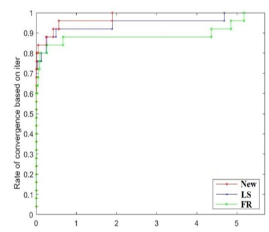
• Figure 1 illustrates the percentage P of test issues resolved within a specified the number of iterations, emphasizing the efficacy of each strategy.
• Figure 2 illustrates the accuracy attained by each method, indicating the number of function evaluations required for convergence.
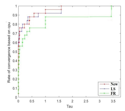
• Figure 3 presents a comprehensive analysis of CPU performance, detailing resource utilization and the scalability of the problem.
The uppermost curve in each figure represents the strategy exhibiting the superior overall performance regarding computing efficiency and accuracy.
The comparative method developed by researchers Dolan and Moré [23], which consisted of generating performance curves for each algorithm, indicated that the proposed method is superior than the traditional methods. The higher the curve, the greater the likelihood that the greatest number of functions will be solved and that the objective will be accomplished.
Figure 1. The efficacy of the comparative algorithms regarding iterations
Figure 2. The efficacy of the comparative algorithms regarding number of function evaluations
Figure 3. The efficacy of the comparative algorithms regarding iterations CPU
5.4 Discussion
We demonstrate how the properties of traditional methods overlap with those of the method that we have invented.
Comparing Mathematically
FR: If we see in Eq. (7), this formula depends only on the norm of the gradients at the current and previous iterations.
LS: As we see in Eq. (8), this formula involves both the gradients and the search direction, potentially providing more information about the problem structure.
New: The vectors used in both formulas include.
Both approaches have the goal of preserving the conjugacy of search directions. However, the LS method is typically seen as more adaptable because it incorporates the search direction dk in its update. Our method certainly achieves this property since we use hybridization.
Both methods have comparable computing complexity, with the main computational task being the evaluation of the gradient and line search. At the same pace of calculations without the expense of the calculations of the gradation and the search line, since we took some balances between the two methods.
The primary differentiation lies in their computation of the parameter beta, which leads to differential features and potential performance attributes.
This article demonstrates the effectiveness of new hybrid conjugate gradient algorithms in solving unconstrained optimization problems by optimizing a new parameter based on the essential quantities extracted from the objective function. Theoretical analyses demonstrate that this method guarantees global convergence. Meanwhile, numerical tests illustrate the superiority of the new algorithms in terms of computational efficiency and convergence speed compared to conventional algorithms. Using the parameters $\beta_k$ and $\theta_k$ indicates the method’s ability to identify effective optimization directions in the solution space, enhancing its suitability for diverse applications. The results demonstrate that the proposed method represents a qualitative addition to the conjugate gradient approach, especially in cases requiring general nonlinear and convex functions unsuitable for global convergence.
This work is being supported by the Ministry of Higher Education and Scientific Research of the Republic of Iraq, as well as the College of Basic Education at the University of Telafer, in partnership with the College of Environmental Sciences and the College of Arts at the University of Mosul.
[1] Jameel, M.S., Abdullah, Z.M., Fawzi, F.A., Hassan, B.A. (2021). A New shifted conjugate gradient method “based” on shifted Quasi-Newton condition. Journal of Physics: Conference Series, 1818: 012105. https://doi.org/10.1088/1742-6596/1818/1/012105
[2] Jameel, M., Al-Bayati, A., Algamal, Z. (2023). Scaled multi-parameter (SMP) nonlinear QN-algorithms. AIP Conference Proceedings, 2845: 060013. https://doi.org/10.1063/5.0157747
[3] AlKawaz, R.Z., AlBayati, A.Y., Jameel, M.S. (2020). Interaction between un updated FR-CG algorithms with optimal cuckoo algorithm. Indonesian Journal of Electrical Engineering and Computer Science, 19(3): 1497-1504. http://doi.org/10.11591/ijeecs.v19.i3.pp1497-1504
[4] Andrei, N. (2020). Nonlinear Conjugate Gradient Methods for Unconstrained Optimization. Springer. https://doi.org/10.1007/978-3-030-42950-8
[5] Fletcher, R., Reeves, C.M. (1964). Function minimization by conjugate gradients. The Computer Journal, 7(2): 149-154. https://doi.org/10.1093/comjnl/7.2.149
[6] Fletcher, R. (1987). Practical Methods of Optimization. John Wiley & Sons.
[7] Conjugate gradient methods. WIKIPEDIA The Free Encyclopedia. https://en.wikipedia.org/wiki/Conjugate_gradient_method.
[8] Hestenes, M.R., Stiefel, E. (1952). Methods of conjugate gradients for solving linear systems. Journal of research of the National Bureau of Standards, 49: 409-435. https://doi.org/10.6028/JRES.049.044
[9] Liu, Y., Storey, C. (1991). Efficient generalized conjugate gradient algorithms, part 1: Theory. Journal of Optimization Theory and Applications, 69: 129-137. https://doi.org/10.1007/BF00940464
[10] Polak, E., Ribiere, G. (1969). Note sur la convergence de méthodes de directions conjuguées. ESAIM: Mathematical Modelling and Numerical Analysis-Modélisation Mathématique et Analyse Numérique, 3(16): 35-43. https://doi.org/10.1051/m2an/196903R100351
[11] Dai, Y.H., Yuan, Y. (1999). A nonlinear conjugate gradient method with a strong global convergence property. SIAM Journal on optimization, 10(1): 177-182. https://doi.org/10.1137/S1052623497318992
[12] Abdullah, Z.M., Jameel, M.S. (2019). Three-term conjugate gradient (TTCG) methods. Journal of Multidisciplinary Modeling and Optimization, 2(1): 16-26.
[13] Malik, M., Mamat, M., Abas, S.S., Sulaiman, I.M. (2020). A new coefficient of the conjugate gradient method with the sufficient descent condition and global convergence properties. Engineering Letters, 28(3): 1-11.
[14] Touati-Ahmed, D., Storey, C. (1990). Efficient hybrid conjugate gradient techniques. Journal of Optimization Theory and Applications, 64: 379-397. https://doi.org/10.1007/BF00939455
[15] Jiang, X.Z., Jian, J.B. (2019). Improved Fletcher–Reeves and Dai–Yuan conjugate gradient methods with the strong Wolfe line search. Journal of Computational and Applied Mathematics, 348: 525-534. https://doi.org/10.1016/j.cam.2018.09.012
[16] Zhao, L.D., Lo, S.H., He, J.Q., Li, H, et al. (2011). High performance thermoelectrics from earth-abundant materials: Enhanced figure of merit in PbS by second phase nanostructures. Journal of the American Chemical Society, 133(50): 20476-20487. https://doi.org/10.1021/ja208658w
[17] Zhang, L., Zhou, W. J. (2008). Two descent hybrid conjugate gradient methods for optimization. Journal of Computational and Applied Mathematics, 216(1): 251-264. https://doi.org/10.1016/j.cam.2007.04.028
[18] Al-Bayati, A.Y., Jameel, M.S. (2014). New Scaled proposed formulas for conjugate gradient methods in unconstrained optimization. AL-Rafidain Journal of Computer Sciences and Mathematics, 11(2): 25-46. https://doi.org/10.33899/csmj.2014.163748
[19] Hestenes, M.R. (1980). Conjugate Direction Methods in Optimization. Springer New York, NY. https://doi.org/10.1007/978-1-4612-6048-6
[20] Jameel, M.S., Abdullah, Z.M., Fawzi, F.A., Hassan, B.A. (2021). A new shifted conjugate gradient method based on shifted quasi-newton condition. Journal of Physics: Conference Series, 1818: 012105. https://doi.org/10.1088/1742-6596/1818/1/012105
[21] Gill, P.E., Murray, W., Wright, M.H. (2019). Practical Optimization. Society for Industrial and Applied Mathematics. https://doi.org/10.1137/1.9781611975604
[22] Aziz, R.F., Younis, M.S., Jameel, M.S. (2024). An Investigation of a new hybrid conjugates gradient approach for unconstrained optimization problems. Bilangan: Jurnal Ilmiah Matematika, Kebumian dan Angkasa, 2(4): 11-23. https://doi.org/10.62383/bilangan.v2i4.136
[23] Dolan, E.D., Moré, J.J. (2002). Benchmarking optimization software with performance profiles. Mathematical Programming, 91: 201-213. https://doi.org/10.1007/s101070100263