Mohamed Jasim Mohamed![]() | Layla H. Abood*
| Layla H. Abood*![]()
Copyright: ©2025 The authors. This article is published by IIETA and is licensed under the CC BY 4.0 license (http://creativecommons.org/licenses/by/4.0/).
OPEN ACCESS
In this study different schemes of Fractional Order PID (FOPID) controllers are suggested to maintain the Automatic Voltage Regulator (AVR), the controllers’ gains are selected using Gorilla Troops Optimization (GTO) and the fitness function Integral Time Absolute Error (ITAE) is used to monitor and obtain the efficient system behavior. The transient analysis is adopted to adjust and obtain the desired response. the nonlinear FOPID faces these signals with a small period and lowest settling time 0.164 sec., it is superior to conventional FOPID by 75.226% and superior to arctan FOPID by 81.898% in simulation time equal to 5 seconds, it reaches its peak value fast (t=0.126 seconds) with a very small value equal to 0.00103 then it will obey the system to a stable level of its desired response efficiently, then the robustness analysis's are tested by adding two external disturbances signals with values equal to ±0.3 v, the three controllers suggested conventional FOPID, arctan FOPID, and the nonlinear FOPID controller try to fix the deviation done by these signals, the nonlinear FOPID faces these signal with small time till reach to the stable desired values. The second one is utilized by varying the original gains model for two parts of the system amplifier and sensor to ±25% from its real value, the best performance also appeared in the nonlinear controller if compared to the other two controllers in adjusting the system response in a small period of time.
Automatic Voltage Regulator system, Fractional Order PID, Gorilla Troops Optimization, Integral Time Absolute Error, terminal voltage
An important matter in any electric device or machine is to obtain a stable and regulated supply voltage. To achieve this requirement the AVR system is adopted for adjusting the voltage to stable desired values by ensuring the supply voltage from the generators and checking its stability continuously. AVR control system stability is a necessary matter for keeping electrical machines and devices connected by maintaining any variations that may happen due to these different studies now available for adjusting AVR system working principles to achieve the best behavior [1, 2]. Many researchers suggested different controllers for controlling and regulating the terminal voltage of the AVR system either by using the conventional PID controller due to its simple scheme or by adding any new optimization algorithms found nowadays. Govindan [3] suggested PID control tuned with a tree seed algorithm, and Pachauri [4] used a water cycle algorithm with PID controller, in the study conducted by Bingul and Karahan [5], a cuckoo search tuning method is used for select the gains for the PID controller to control system. Micev et al. [6] suggested a structure from PID plus second-order derivative to enhance system behavior, other studies adopt the idea of using Fractional calculus techniques by adding two new parameters (λ, μ) [7, 8] that can improve the system performance and stability as in the study [9] a FOPID controller is adopted with a modified Gray wolf optimization and Khan et al. [10] used also a FOPID with a salp swarm optimization algorithm which enhances the efficiency and the system stability other studies use the fuzzy logic technique as Mazibukol et al. [11] used the fuzzy logic controller for enhance system dynamics and achieve a stable terminal voltage while Eltag and Zhang [12] suggested using the fuzzy logic controller with the classical PID type for maintaining the AVR system regulating principles by fix the weakness appeared when using a classical controller especially when there is a disturbance signal that influences on system behavior.
In this paper an AVR system is controlled by using three suggested controller (FOPID, NLFOPID, arctan FOPID) based on using different schemes of FOPID, it can be seen that these various controllers give a fast response represented by its settling time values and stable behavior with an acceptable levels of undershoot or overshoot values appeared at the starting time of simulation period then reach to a regular stable response with a smart GTO algorithm for the improvement of AVR system and regulating its supplied voltage when its compared with the previous studies demonstrated in the survey, then two types of robustness analysis are presented to test AVR system behavior, first test is using an external disturbance signals in different specific periods while the second one is utilized by varying two gains values (amplifies & sensor gain values) by ±25% from its original value for all suggested controller to indicate the controller robustness depending on its evaluation parameters used.
This study is arranged as listed: Section 2 describes the AVR system modeling, and Section 3 demonstrates the proposed schemes of the FOPID controller. Section 4 presents the GTO tuning method for finding the suitable controller parameters, Section 5 discusses the results obtained in the simulation, and the conclusion points are shown in Section 6.
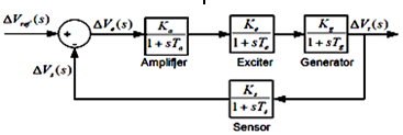
The essential issue in using AVR system is regulating the terminal voltage of the generator by maintaining the excitation system. The system has four parts: amplifier, exciter, generator, and sensor as shown in Figure 1, each part has a transfer function with a typical value as explained in Table 1, the values of the AVR system chosen are as follows: Ka=10, Ke=1, Kg=1, Ks=1, Ta=0:1, Te=0:4, Tg=1, Ts=0:01. The values adopted in this study are the most used values in the literature [3, 8].
Figure 1. The AVR system model
Table 1. AVR parts transfer function
|
AVR Part |
Transfer Function |
|
Amplifier |
$\frac{\mathrm{Ka}}{s T a+1}$ |
|
Exciter |
$\frac{\mathrm{Ke}}{s T e+1}$ |
|
Generator |
$\frac{\mathrm{Kg}}{s T g+1}$ |
|
Sensor |
$\frac{\mathrm{Ks}}{s T s+1}$ |
The overall transfer function will be [3]:
$\frac{V t(s)}{V re f(s)}=\frac{0.1 s+10}{0.0004 s^4+0.0454 s^3+0.555 s^2+1.51 s+11}$ (1)
3.1 Conventional FOPID controller with derivative filter
The FOPID controller is a type of controller regarded as an enhanced scheme for the PID classical controller type that uses the integration and differentiation in any order, while FOPID (or PIlDm) controller is different from PID in using fraction numbers for these two actions as shown in the controller equation [13] and its structure is in Figure 2.
Figure 2. Conventional FOPID controller with derivative filter
$u(t)=K_p e(t)+K_i D^{-\lambda} e(t)+K_d D^\mu \frac{N}{D+N} e(t)$ (2)
3.2 Arctan FOPID controller with derivative filter
The use of some mathematical functions like hyperbolic or trigonometric functions will improve the system response and lead to accurate and stable behavior [14] for this reason various studies adopt these types of equations reach to the desired and stable response, in this paper the second controller adopts the arctan FOPID which is utilized by changing the integral part in its structure from integrating the error to integrates the arctan function of the system error, as indicated in its relation. This type of controller is better than the conventional PID in attenuating the non-constant disturbance, its relation appears in Eq. (3) [15].
While the arctan FOPID control law is described by equation:
$u(t)=K_p e(t)+K_i D^{-\lambda} tan ^{-1}(\gamma e(t))+K_d D^\mu \frac{N}{D+N} e(t)$ (3)
where, γ is the design parameter.
3.3 The nonlinear FOPID controller with derivative filter
The use of NLPID type has been adopted to achieve a set and satisfied response for the nonlinearity in issue in nonlinear systems, where it is used in all terms of the normal controller a nonlinear relation f(.) consists of a nonlinear combination of [sign & exponential] relations of the system error as indicated below:
$u(t)=f_1(e)+f_2(\dot{e})+f_3\left(\int e \,\,d t\right)$ (4)
$k_n(\beta)=k_{n 1}+\frac{k_{n 2}}{1+exp \left(\mu_n \beta^2\right)}$, for $n=1,2,3$ (5)
$f_n(\beta)=k_n(\beta)|\beta|^{a_n} {sign}(\beta)$ (6)
where, $\beta$ could be $e, \dot{e}$, or $\int e\,\, dt, \alpha_i \in R^{+}$, the function $k_n(\beta)$ is a gain with coefficients $k_{n 1}, k_{n 2}, \mu_{n 1} \in R^{+}$. For increasing the NLPID controller response to any value of errors, the nonlinear term $k_n(\beta)$ is used for small errors close to zero; while the term $k_n(\beta)$ value approaches the upper bound $k_{n 1}+k_{n 2} / 2$. In large values of errors, the adopted nonlinear term $k_n(\beta)$ reaches the lower values bound of $k_{n l}$, this indicates that the nonlinear gain term $k_n(\beta)$ is bounded in the sector $\left[k_{n 1}, k_{n 1}+\frac{k_{n 2}}{2}\right]$.
The equations of the proposed NLFOPID controller are shown below [16]:
$e(t)={input}(t)- output (t)$ (7)
The proportional term is:
$\beta_1=e(t)$ (8)
$\left.k_P\left(\beta_1\right)\right)=k_{p 1}+\frac{k_{p 2}}{1+exp \left(\mu_p \beta_1^2\right)}$ (9)
$f_p\left(\beta_1\right)=k_p\left(\beta_1\right)\left|\beta_1\right|^{\alpha_p} {sign}\left(\beta_1\right)$ (10)
The Integral term is:
$\beta_2=D^{-\lambda} e(t)$ (11)
$k_i\left(\beta_2\right)=k_{i 1}+\frac{k_{i 2}}{1+exp \left(\mu_i \beta_2^2\right)}$ (12)
$f_i\left(\beta_2\right)=k_i\left(\beta_2\left|\beta_2\right|^{\alpha_i} {sign}\left(\beta_2\right)\right.$ (13)
The derivative term is:
$\beta_3=D^\mu \frac{N}{D+N} e(t)$ (14)
$k_d\left(\beta_3\right)=k_{d 1}+\frac{k_{d 2}}{1+exp \left(\mu_d \beta_3^2\right)}$ (15)
$f_d\left(\beta_3\right)=k_d\left(\beta_3\right)\left|\beta_3\right|^{\alpha_d} {sign}\left(\beta_3\right)$ (16)
The control action is:
$u(t)=f_p\left(\beta_1\right)+f_i\left(\beta_2\right)+f_d\left(\beta_3\right)$ (17)
Optimization algorithms become a helpful way to solve various problems because in our lives, all creatures are organized as a smart collective group, and the behavior of these groups is interpreted and programmed into an efficient algorithm [17]. Artificial Gorilla Troops Optimizer (GTO) is one of the most useful algorithms. They are arraigned and collected as troops; adult mothers with their small children of gorilla are controlled and obey an adult gorilla male with silver hair color named the silverback father. All families wish to go out from their troop to another one, the males of each troop always try to follow another troop by drawing attention to the females in the new troop group but some males prefer to stay were born and obey their silverback troop. When the adult responsible leader gorilla dies, all gorillas that prefer to not leave their troop will either be presented to lead the troop or suggested to be controlled by the silverback. In the algorithm, the leader which is the adult one is considered as the suitable solution(optimal), while other males will follow him and discard the weakest gorilla (not optimal), two phases represent this behavior. GTO was inspired by gorillas' social intelligence and collective lifestyle. According to exploratory studies, GTO carries out well in the extreme when selected to tune different variables in various engineering fields. Like other optimization methods, it will tend to get stuck in the local optimum when solving complex optimization problems also it still has low optimization accuracy and converges too quickly.
4.1 Exploration stage
In this stage, the gorilla population is considered as a competitor for finding the decision suggested by the silverback adult gorilla. Three decisions are specified here and shown in. eq. (18) below, the first decision is to raise exploration of the GTO by emigration to uncharted positions while the second is to poise the exploitation and exploration by emigrating to different troops, and then the final decision is for raising GTO capability for finding in other positions by emigrating to known position.
$\begin{aligned}
& G X(t+1)
=\left\{\begin{array}{c}
(U L-L L) r_{-} 1+L L, { if~rand }<P \\
\left(r_2-a\right) X_r(t)+L \times H, { if~rand } \geq 0.5 \\
X(i)-L\left(L\left(X(t)-G X_r(t)\right)+r_3\left(X(t)-G X_r(t)\right)\right), { if~ rand }<0.5
\end{array}\right.
\end{aligned}$ (18)
The current position is the vector (t), "GX(t+1)" selects the location for the next iteration. The parameter Xr(t) is adapted to any one elects of the troop randomly selected from the troop and GXr(t) is the random gorilla place. UL and LL are the parameter bands (upper & Lower), and the values r1, r2, and r3 are chosen randomly from 0 to 1. The other variables like a, L, and H are found as indicated below:
$a=C \times(1-I t / M a x I t)$ (19)
$C=cos \left(2 \times r_4\right)+1$ (20)
$L=c \times l$ (21)
$H=Z \times X(t)$ (22)
$Z=[-a, a]$ (23)
4.2 Exploitation stage
In this stage two selected decisions are available, one obeys the adult gorilla silverback while the other must enter the contest for the adult available females, each decision is evaluated by comparing the a variable in Eq. (23), if it is greater or equal W, the first one is chosen, but if less than W, and the second one is chosen. W is a known value and is given before the algorithm starts.
4.2.1 Obeying the adult silverback gorilla
In this choice, silverback one is the leader, while gorilla population takes his opinions to discover their source of food, it is adopted if a≥w and its relations are as indicated below:
$G X(t+1)=L \times M \times\left(X(t)-X_{{silverback }}\right)+X(t)$ (24)
where, Xsilverback is the point where the silverback is placed, and X(t) is the normal gorilla position; the L and M values are chosen.
4.2.2 Adult females’ competition
This selection here from the males that are regarded as a young one that accomplish puberty age, contest here is very harmful due to the fight between them to comprise new troops after electing a new female adult age. This decision is taken when a<w and it is found based on the equations below:
$G X(i)=X_{{silverback }}-\left(X_{{silverback }} \times R-X(t) \times R\right) \times A$ (25)
$R=2 \times r_5-1$ (26)
$A=\beta \times E$ (27)
$E=\left\{\begin{array}{l}N_1={ rand } \geq 0.5 \\ N_2={ rand }<0.5\end{array}\right.$ (28)
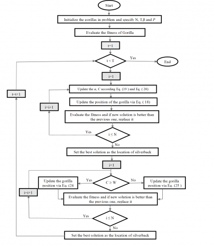
where, R represents the impact force, it can be found using Eq. (20), r5 is chosen randomly between [0,1], if a conflict appears, Eq. (23) is adopted for finding the harm level in conflicts and A is the vector that is suggested for finding the harm value and it is obtained based on Eq. (21). A number of predetermined parameters like a, β, E is regarded as the harm effect on the decision boundaries. And then the index function value of all GX(t) is found, if the index value of GX(t)<X(t), the GX(t) selects X(t) as an optimal selection between the population and is regarded as a leader (silverback). Figure 3 explains the steps of GTO algorithm.
Figure 3. GTO algorithm steps
In this part of the paper, all simulation analyses of the AVR system for the three optimal controllers are demonstrated. The proposed controller's schemes are simulated using the MATLAB 2019 program, and the simulation time is 5 seconds. The controllers are adjusted to achieve the best response wanted; the analysis is done with the benefits of using a suitable cost function.
Table 2. GTO variables
|
Description |
Value |
|
Gorilla numbers |
50 |
|
Maximum iteration |
30 |
|
Dimension (tuned variables) |
(6-14) |
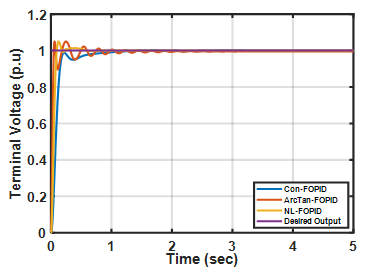
Figure 4. AVR system response for all controllers
These controllers are tested and analyzed to achieve the best and most stable system behavior using GTO as a tuning method, Table 2 explains the variables of the GTO algorithm, and Figure 4 describes the system block diagram.
Figure 4 is a drawing for controlled AVR based on the GTO algorithm. For testing error value continually [18] and monitoring response performance to obtain the robust and stable level of selected terminal voltage, an ITAE fitness function indicated in Eq. (29) is used [19] to check the error while GTO is run until choosing the tuned parameters (gains) and reached to a stable response [20], in Figure 5, the system response for the suggested controllers.
$I T A E=\int_0^{\infty} t|e| d t$ (29)
The tuned gains obtained for all controllers are listed in Table 3. Table 4 indicates the evaluation parameters which are listed to assess the controller's performance.
Table 3. Controllers tuned gains
|
Controller Type |
Kp |
Ki |
Kd |
N |
μ |
λ |
γ |
|
Con_FOPID |
2.15577 |
10.0 |
0.31515 |
84.47909 |
-1.0111 |
1.41238 |
- |
|
Arctan_FOPID |
2.78146 |
4.09198 |
0.52552 |
100.0 |
-0.00547 |
1.821078 |
50.0 |
|
NL_FOPID |
$K_{p 1}$ |
$K_{i 1}$ |
$K_{d 1}$ |
|
|
1.59346 |
- |
|
|
|
0.04889 |
0.415477 |
100.0 |
|
|
|
|
0.69999 |
|
|
|
-1.390011 |
|
|
|
|
|
$K_{i 2}$ |
$K_{d 2}$ |
|
|
|
|
|
|
$K_{p 2}$ |
2.22673 |
4.157706 |
|
|
|
|
|
|
|
$\mu_i$ |
$\mu_d$ |
|
|
|
|
|
|
8.61480 |
0.11142 |
0.027192 |
|
|
|
|
|
|
$\mu_p$ |
$\alpha_i$ |
$\alpha_d$ |
|
|
|
|
|
|
0.000 |
0.11062 |
1.000 |
|
|
|
|
|
|
$\alpha_p$ |
|
|
|
|
|
|
|
|
0.36323 |
|
|
|
|
|
|
Table 4. Results of all suggested controllers
|
Controller Type |
Rise Time |
Over Shoot/Under Shoot % |
Peak Time |
Settling Time |
Steady State Error |
ITAE |
|
Con_FOPID |
0.195 |
0.108 |
2.954 |
0.662 |
0.001959 |
0.022228175 |
|
Arctan_FOPID |
0.047 |
4.99/10.03 |
0.248/0.113 |
0.906 |
0.00559 |
0.074295722 |
|
NL_FOPID |
0.092 |
4.930 |
0.126 |
0.164 |
0.00103 |
0.005698963 |
Figure 5. AVR system response for all controllers
In Table 4, it can be seen that:
-The Nonlinear FOPID (NL- FOPID) controller has a superior behavior if it's compared with the conventional and the arctan FOPID controllers suggested.
- It has a small rise time with a value equal to 0.092 sec., an overshoot appears at the start of its work but it is still the best in reaching the desired response with a small value of its settling time (0.164 sec.).
-A small steady-state error equal to 0.00103, also a small ITAE (0.005698963)
When analyzing the other two controllers used in comparison it can be seen that the conventional controller does not have a higher overshoot value but it suffers from the higher value of its rise time (0.195) and also a higher settling time value equal to 0.662 while the arctan FOPID suffer from higher value of overshoot and undershoot (4.99/10.030) and higher settling time value 0.906 due to all this, the NL-FOPID can be selected as the most suitable choice for maintaining the terminal voltage value in the AVR system.
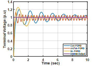
The robustness analysis is utilized for checking system behavior, it is done in two steps; the first step is changing the system parameters gains for two parts in AVR system model(amplifier and sensor), this change in values may happen due to different matters like component damage or increase the load during work, a ±25% from its normal values, while the second step is by applying two disturbances, signals positive and negative signal values (±0.3 volt) that added suddenly from external environment, this case happen when increase the load without modifying the component used based on this change done or a non-regular power is supplied from the supply network system due to a technical error happens, this step is to verify the effectiveness of the suggested used in obtaining the desired value of AVR system, the system behavior is shown in Figure 6 for the first power reached from the supply network system step and for the second step is appeared on Figure 7.
The second step is shown in Figure 7 as shown unexpected deviation is happened to the voltage value in negative and positive values in its desired level due to the external disturbances signal that may cause by any matter in the environment where the AVR system is used, these signals values is (±0.3 volt) in two periods of time as explained in Figure 7.
(a)
(b)
(c)
(d)
Figure 6. (a) -25% in amplifier gain; (b) +25% in amplifier gain; (c) 25% in sensor gain; (d) +25% in sensor gain amplifier
(a)
(b)
Figure 7. (a) Add positive value=+0.3 volt at t=3 sec; (b) Add negative value=-0.3 volt at t=2 sec
In this study a different robust structure of FOPIDs is suggested, all these structure gains are found using GTO tuning method, and this smart algorithm and ITAE cost function are used to select the suitable values of all controller parameters to reach a stable and robust system response. The fractional calculus and the nonlinear functions improve system stability and behavior as shown in the evaluation parameters used when comparing between suggested controllers. The robustness tests are used for all suggested controllers to check the stability of the system and to check its ability to reject disturbances that may happen during working, the changing of system parameters values by ±25% is done for all controllers and as shown the nonlinear FOPID is superior to other controller in led the system to return to its acceptable value in a small period between 0.5-3.6 sec. which is regarded as a small value and may not sense in the second test when applied ±0.3 v, the nonlinear also faces these signals with an acceptable value of overshot I the positive value, or undershoot in the negative value and leads the system to a stable level in a small period of time equal to 1.3 sec when adding positive disturbance signal and 1.7 sec. When adding a negative disturbance signal the system response will have an overshoot in its behavior, after 0.5 sec. the system reaches its desired behavior then negative and positive disturbance signals are applied to the system, the controllers affected by these signals then within 0.25 sec the system behavior reaches its acceptable values. Numerical results showed that the nonlinear controller is robust enough to control the value of the AVR terminal voltage. In future work, a suggestion can be made by using a cascade scheme with a neurocontroller or sliding mode controller also can use recent optimization algorithms that can help in finding more accurate values for controller variables to enhance system performance.
[1] Mahmood, S.A., Humod, A.T., Issa, A.H., Ameen, N.M. (2023). Robust AVR based on augmented PI controller for synchronous generator. AIP Conference Proceedings, 2804(1): 030005. https://doi.org/10.1063/5.0154585
[2] Abood, L.H., Mohamed, M.J., Abood, M.H. (2023). A Dual-stage optimal controller design for controlling AVR system. In 2023 27th International Computer Science and Engineering Conference (ICSEC), pp. 122-126. https://doi.org/10.1109/ICSEC59635.2023.10329680
[3] Govindan, P. (2020). Evolutionary algorithms-based tuning of PID controller for an AVR system. International Journal of Electrical & Computer Engineering, 10(3): 3047-3056. https://doi.org/10.11591/ijece.v10i3.pp3047-3056
[4] Pachauri, N. (2020). Water cycle algorithm-based PID controller for AVR. COMPEL-The International Journal for Computation and Mathematics in Electrical and Electronic Engineering, 39(3): 551-567. https://doi.org/10.1108/COMPEL-01-2020-0057
[5] Bingul, Z., Karahan, O. (2018). A novel performance criterion approach to optimum design of PID controller using cuckoo search algorithm for AVR system. Journal of the Franklin Institute, 355(13): 5534-5559. https://doi.org/10.1016/j.jfranklin.2018.05.056
[6] Micev, M., Ćalasan, M., Radulović, M. (2021). Optimal design of real PID plus second-order derivative controller for AVR system. In 2021 25th International Conference on Information Technology (IT), pp. 1-4. https://doi.org/10.1109/IT51528.2021.9390145
[7] Abood, L.H., Ali, I.I., Oleiwi, B.K. (2022). Design a robust fractional order TID controller for congestion avoidance in TCP/AQM system. In 2022 26th International Computer Science and Engineering Conference (ICSEC), pp. 366-370. https://doi.org/10.1109/ICSEC56337.2022.10049311
[8] Kadhim, N.N., Abood, L.H., Abd Mohammed, Y. (2023). Design an optimal fractional order PID controller for speed control of electric vehicle. Journal Européen des Systèmes Automatisés, 56(5): 735-741. https://doi.org/10.18280/jesa.560503
[9] Verma, S.K., Devarapalli, R. (2022). Fractional order PIλDμ controller with optimal parameters using Modified Grey Wolf Optimizer for AVR system. Archives of Control Sciences, 32(2): 429-450.
[10] Khan, I.A., Alghamdi, A.S., Jumani, T.A., Alamgir, A., Awan, A.B., Khidrani, A. (2019). Salp swarm optimization algorithm-based fractional order PID controller for dynamic response and stability enhancement of an automatic voltage regulator system. Electronics, 8(12): 1472. https://doi.org/10.3390/electronics8121472
[11] Mazibukol, N., Akindejil, K.T., Sharma, G. (2022). Implementation of a FUZZY logic controller (FLC) for improvement of an Automated Voltage Regulators (AVR) dynamic performance. In 2022 IEEE PES/IAS PowerAfrica, pp. 1-5. https://doi.org/10.1109/PowerAfrica53997.2022.9905407
[12] Eltag, K., Zhang, B. (2021). Design robust self-tuning FPIDF controller for AVR system. International Journal of Control, Automation and Systems, 19: 910-920. https://doi.org/10.1007/s12555-019-1071-8
[13] Ibrahim, E.K., Issa, A.H., Gitaffa, S.A. (2022). Optimization and performance analysis of fractional order PID controller for DC motor speed control. Journal Européen des Systémes Automatisés, 55(6): 741. https://doi.org/10.18280/jesa.550605
[14] Ali, E.H., Reja, A.H., Abood, L.H. (2022). Design hybrid filter technique for mixed noise reduction from synthetic aperture radar imagery. Bulletin of Electrical Engineering and Informatics, 11(3): 1325-1331. https://doi.org/10.11591/eei.v11i3.3708
[15] Al-samarraie, S.A., Abbas, Y.K. (2012). Design of electronic throttle valve position control system using nonlinear PID controller. International Journal of Computer Applications, 59(15): 27-34.
[16] Najm, A.A., Ibraheem, I.K. (2019). Nonlinear PID controller design for a 6-DOF UAV quadrotor system. Engineering Science and Technology, 22(4): 1087-1097. https://doi.org/10.1016/j.jestch.2019.02.005
[17] Hadi, M.H., Issa, A.H., Sabri, A.A. (2023). Improvement of salp swarm algorithm (SSA2) for intelligent fault detection in smart wireless sensor networks. Materials Today: Proceedings, 80: 3322-3327. https://doi.org/10.1016/j.matpr.2021.07.248
[18] Shneen, S.W., Dakheel, H.S., Abdulla, Z.B. (2016). Advanced optimal for PV system coupled with PMSM. Indonesian Journal of Electrical Engineering and Computer Science, 1(3): 556-565.
[19] Abdollahzadeh, B., Soleimanian Gharehchopogh, F., Mirjalili, S. (2021). Artificial gorilla troops optimizer: A new nature‐inspired metaheuristic algorithm for global optimization problems. International Journal of Intelligent Systems, 36(10): 5887-5958. https://doi.org/10.1002/int.22535
[20] Mahmood, Z.N., Al-Khazraji, H., Mahdi, S.M. (2023). Adaptive control and enhanced algorithm for efficient drilling in composite materials. Journal Européen des Systèmes Automatisés, 56(3): 507-512. https://doi.org/10.18280/jesa.560319