Mohamed Abdulrahman Abdulhamed*![]() | Asaad Noori Hashim
| Asaad Noori Hashim![]()
© 2025 The authors. This article is published by IIETA and is licensed under the CC BY 4.0 license (http://creativecommons.org/licenses/by/4.0/).
OPEN ACCESS
Recent research has shown that videos created using generative adversarial networks have visible imperfections that significantly diminish the overall quality of the synthetic videos. However, counterfeit deepfake samples have dramatically increased, resulting in near-perfect replicas of reality that can easily deceive the human eye. These technologies threaten society and individuals on multiple fronts, including sociological, religious, and political dimensions. The primary objective of this study is to undertake several analyses, including inferential statistics, quality assessments (noise), similarity assessments (structure and correlation), and testing utilizing machine learning models. Eight different machine learning techniques were employed, including Support Vector Classifier (SVC), Random Forest (RF), and XGBoost, with the extracted features included. In a statistical feature analysis, the Bagging classifier outperformed the others. Accuracy, F1-score, and AUC scores were 0.722, 0.725, and 0.722, respectively. Thus, analyzing the causes before suggesting detection methods may help solve challenging computer vision problems, such as the deepfake problem. On this basis, we customize a convolutional neural network. This network was trained using FaceForensics++ (FF++) samples and has a 97% accuracy rate.
generative adversarial networks, machine learning, deep learning, generative adversarial networks, behaviors, inferential statistics
The efficiency of audio, video, and image processing technologies has significantly improved due to the rapid development of advanced technologies, such as artificial intelligence, cloud computing, and GPU devices. Additionally, the emergence of advanced machine learning (ML) approaches, such as generative adversarial networks (GANs), has further contributed to this development. Accordingly, various forms of media emerged. This development has given rise to a new phenomenon known as artificially generated media, produced through advanced artificial intelligence, commonly referred to as ‘deepfakes’ [1].
Deepfakes and GANs can generate synthetic data that resemble real media, which can be used for good or evil. Although technologies have become practical communication tools, the lack of regulation makes them more susceptible to widespread production and dissemination. These technologies can damage reputations, deceive the public, and undermine democratic processes. Identification of social media-manipulated films has become increasingly challenging, especially with the advancement of deepfakes [2, 3]. An example of a low-cost counterfeit is the video titled “Drunk Pelosi” [4].
The most challenging issues in addressing the problem of deep fake detection are generalizability, robustness, and lack of interpretability [5, 6]. Accordingly, this study focuses on the latter problem, utilizing a systematic analytical approach from several perspectives to identify the key characteristics that could aid in developing practical and comprehensive deep fake detection models.
Inferential statistical approaches are used to analyze deepfake datasets, focusing on hypotheses and differences between samples. Hypothesis testing is a fundamental method involving formulating hypotheses about population parameters and evaluating their plausibility. It can be used to compare characteristics like visual quality and detection accuracy between deepfake and non-deepfake samples. To prove the hypothesis that statistical significance exists between real video samples processed using generative adversarial networks is the main objective of using it in our proposed study.
The research methodology is as follows: Firstly, we start with inferential statistical approaches because they affect data direction, nature, and variation. This approach may help provide statistical significance to differentiate between real and fake samples [7]. ANOVA compares authentic and counterfeit samples in a standard distribution test. This method compares data to normal distributions using p-values and test statistics to determine confidently. Normal distribution tests improve analysis accuracy and study interpretation. This study attempts to draw valid conclusions about the populations under study using statistical approaches that assume a normal distribution [8]. After that, similarity metrics, such as the structural similarity index (SSIM) and correlation coefficients, quantify data representation similarity. SSIM compares local patterns of pixel intensities normalized for brightness and contrast to estimate the visual similarity between images based on luminance, contrast, and structural information. Correlation coefficients, such as Pearson’s r, measure the linear relationships between quantitative variables. SSIM also evaluates data for perceptual similarities, while correlation finds functional links in multivariate data [9]. Furthermore, the features derived from the aforementioned analytic methods must be evaluated using a set of well-known machine-learning algorithms commonly used for binary classification tasks [10, 11].
Convolutional neural networks (CNNs) can improve binary classification performance through various means. Extensive data augmentation can expose the model to a broader range of input changes during training. Rotations, shifts, and flip train data to generate more synthesized samples. Dropout and L2 weight decay prevent overfitting and promote generalizability. CNNs can learn more discriminative features by optimizing convolutional filter sizes and layer numbers based on input properties and issue difficulty. The receiver operating characteristic (ROC) curve must be monitored to maximize the F1-score, and the classification threshold must be adjusted based on the desired precision-recall tradeoff [12].
The problem statement can be summarized as follows: there is currently no efficient method to identify deepfake samples of various kinds, which is known as a generalized issue [13]. As a result, the techniques used to create and detect deepfakes differ significantly. We studied generative adversarial algorithm instances before creating machine learning models to build more efficient and accurate detection systems. Current deepfake detection methods lack this. This work aims to study the factors that contribute to the extraction of statistical features that may have statistical significance in distinguishing between real and fake samples. The scope of the investigation is limited to samples of the FaceForensics++ (FF++) dataset.
The remainder of this article is organized as follows: Section 2 presents the related work, a series of studies for the detection of fake videos that have been proposed in recent years based on analytical methods. Section 3 is an overview of the vital study concepts, followed by the methodology used during the study in Section 4. Section 5 presents the results and their discussion. Finally, Section 6 provides the conclusions and recommendations for future directions.
The contributions of our study are summarized as follows:
• Propose a method for identifying the region of interest and the most significant influence in the resulting deepfake samples;
• The procedure also included preparing and organizing a video dataset from FF++ data. The clips are created to capture and delineate the facial area with consistent accuracy, regular time intervals, and a pre-determined number of frames, allowing researchers to conduct studies without preprocessing.
• Statistical analysis files are produced using the FF++ dataset to depict the statistical behavior of the dataset.
• An alternative hypothesis was proposed and confirmed through statistical analysis, which may encourage further exploration in this direction to develop models for deepfake detection.
• The dataset was analyzed using eight distinct machine-learning algorithms.
• A deep learning model was proposed to detect deepfake videos using custom CNNs, which achieved high accuracy rates.
Deepfake content is created in a way that can be challenging for humans to detect. Accordingly, researchers have proposed various methods, including ML algorithms and deep learning techniques, to identify discrepancies, distortions, and artifacts in the resulting content. In this section, we will discuss some articles related to our research topic.
Li [14] introduced a deep learning technique for differentiating between artificially made phony videos and authentic ones. The approach uses convolutional neural networks (CNNs) to detect unique characteristics in affine face warping, a technique frequently employed in deepfake films originating from many origins. This approach offers a more efficient and resilient alternative to earlier techniques by reducing the time and resources required for training data sets. The approach is assessed on two sets of deepfake video datasets (deepfake video dataset UADFV and deepfakeTIMIT) to determine its practical efficacy. Unlike other approaches, your method prioritizes a particular intuitive factor in creating deepfake videos, specifically the irregularities in resolution seen in face warping. When faced with deepfake videos from different sources, this specific emphasis increases the robustness of your approach. While Head Pose depends on changes in head pose to differentiate between real and altered videos, this physical cue might not be as noticeable when handling frontal faces.
Marra et al. [15] discovered that every GAN produces a distinct pattern in the images it creates, which can be highly useful for forensic investigations. The study mentioned above aims to establish the presence of GAN fingerprints and their significance in ensuring dependable forensic examinations. Additionally, the study raises inquiries about intriguing subjects that necessitate future exploration. Subsequent research is essential to evaluate the capabilities of GAN fingerprints in the field of multimedia forensics. This work includes determining their effectiveness in distinguishing between authentic photos and those generated by GANs, identifying the origin of GAN-generated content, and understanding how a variety of factors, such as image dimensions and quantity, influence their performance.
Consequently, this study analyzed visual images rather than videos. The researchers also recommended conducting similar investigations to identify fingerprints left by generative adversarial algorithms. These investigations could make valuable contributions toward addressing specific issues, such as deepfakes.
Gragnaniello et al. [16] examined existing techniques for identifying synthetic media, with a specific emphasis on practical situations, such as the uploading of content on social media and the development of new frameworks. They determined that a reliable means for detecting GAN-generated images is still lacking, primarily due to problems such as misalignment between training and testing data, compression, and scaling. Nevertheless, the analysis highlights crucial components for developing practical solutions and offers suggestions for future research. The recommendation that caught our attention in this study is that further investigations should be undertaken to identify the key components of promising solutions to the deepfake problem, thereby advancing toward more effective strategies.
Guarnera et al. [17] suggested a novel algorithm designed for detecting deepfakes in human face images. The objective of this work is to develop a novel detection technique for identifying forensic evidence concealed inside photographs, similar to a fingerprint left during the image creation process. The method utilizes an expectation maximization (EM) algorithm to extract specific characteristics within the data, which are subsequently utilized to represent the fundamental convoluted generative process. The efficacy of the method was demonstrated through tests conducted on five distinct designs and the utilization of the CELEBA dataset. The fundamental concept assumes that the local correlation of pixels in deepfakes depends solely on the operations of all GAN layers, particularly the (later) transpose convolution layers. Unsupervised ML was used to find these traces. Various unsupervised learning methods aim to cluster input dataset instances with high similarity and high dissimilarity between cluster instances. These clusters may represent the dataset’s ‘hidden’ structure. Thus, the clustering method must estimate the distribution parameters that likely generated the training data.
Giudice et al. [18] presented a novel methodology for identifying GAN-specific frequencies (GSF) in deepfake images, which serve as distinctive characteristics of various generative architectures. The method utilizes discrete cosine transform and beta statistics to identify data generated by GAN engines. The CTF technique is characterized by its speed, interpretability, and lack of need for substantial processing resources during training. The GSF exhibits intriguing characteristics, notably its capacity for providing comprehensible explanations in the context of forensic investigations. A G-boost classifier is used to attain superior accuracy values. The additional analysis offers the potential to identify GAN artifacts and provide details about the re-enactment step. Celeb A and FFHQ facial image datasets were utilized for experiments. However, this study did not analyze the video datasets.
The most common artifact deepfake detection model [19] is an innovative method for detecting deepfakes that focuses on acquiring knowledge about shared artifact characteristics seen in facial modification algorithms. The primary hindrance is implicit identity leakage (IIL), which diminishes the model’s capacity to generalize on unfamiliar datasets. The model acquires proficiency in binary classifiers through the utilization of the artifact detection module (ADM), resulting in a significant reduction in the influence of IIL and surpassing the current highest level of performance. This study offers novel perspectives on the generalization of models in deepfake detection and demonstrates that handcrafted artifact feature detectors are not essential. This study proposes that ADMs identify fraudulent photos by focusing on small artifact areas and taking into consideration the observation that local areas often do not accurately represent the identity of images. The learning process of the model for acquiring the overall identity representation of images can be restricted to mitigate the influence of IIL.
As reported by Mitra et al. [20], a CNN-classifier network model and technique are suggested to reduce deepfake video detection computation. This approach begins with key video frame extraction, followed by CNN and classifier networks. Conclusively, a novel method utilizing neural networks is proposed for the detection of deepfake videos on social media platforms. Subsequently, the model attains a high level of accuracy while demanding fewer processing resources. The outcome yielded a 92.33% accuracy by utilizing a merged dataset consisting of FaceForensics++ and Deepfake Detection Challenge. Limitations in this study include limited social network video tries and stated accuracy in detecting fake videos with one frame.
Wodajo and Atnafu [21] introduced a Convolutional Vision Transformer as a method for detecting deepfakes. This approach involves two main components: a CNN and a VTransformer. The CNN is responsible for extracting characteristics that can be learned, while the transformer takes these learned features as input and uses an attention mechanism to categorize them. The model was trained on the DeepFake Detection Challenge Dataset (DFDC) and achieved an accuracy of 91.5 percent, an AUC value of 0.91, and a loss value of 0.32. Your contribution involves the integration of a CNN module into the VIT architecture, resulting in a commendable performance on the DFDC dataset. They achieved an accuracy rate of 91.5% when performing on the DFDC dataset. The potential application of this research lies in its ability to avoid identity theft and scams. However, the data preprocessing stage, which plays a crucial role in extracting the features used in the proposed model, is not adequately explained.
Deepfake has grown in popularity due to its ability to make realistic images using deep learning and ad-hoc GANs. Accordingly, deepfakes of human faces are analyzed to develop a revolutionary detection method that can discover a forensic trail buried in images akin to a fingerprint left in image generation. Based on the investigations above, most of them achieved the best accuracy results in classification. Nevertheless, it fails to possess the capability to discover efficient machine-learning models for addressing the generalization issue, as indicated by its reliance on particular data sets for training and testing purposes. This discrepancy compels us to seek novel methodologies to enhance the efficacy and robustness of constructing classification models. Where can one undertake in-depth analytical studies to identify the most significant disparities between authentic and counterfeit information produced by sophisticated artificial intelligence. In this work, we used an analytical investigation using multiple elements to find differences that might distinguish fake from authentic information and address the deep fake problem.
Our work used region of interest identification, inferential statistics, and similarity measurements to develop ML models from the data obtained. Therefore, the studies as mentioned above lacked a comprehensive set of systematic analyses. For this purpose, this work aims to develop a fresh strategy for studying the deepfake problem.
Deepfake and other generative artificial intelligence (AI) (GAI) techniques are classified under AI-generated material (AIGC), which encompasses the production of digital material, including images, music, videos, and natural language, using AI models. The objective of AIGC is to enhance the efficiency and accessibility of the content creation process, enabling the generation of top-notch material at an accelerated rate. AIGC is accomplished through the extraction and comprehension of intent information from human-provided instructions and generating content based on its knowledge and the intended information [22].
This section presents a brief overview of the most important basic concepts adopted in conducting the study. Given that many of these concepts have been summarised in the form of tables or illustrations, we have added their sources that can be relied upon for additional details. The justification is to focus on the most important strengths of these popular concepts in the field of computer vision to reduce the reading effort of researchers and save time.
3.1 Conditional GAN
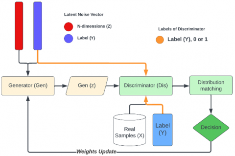
Generative modeling is an unsupervised learning technique in ML that enables the identification and understanding of patterns or regularities in the input data. These patterns may then be utilized to generate new examples or outputs based on the original dataset. GANs are a framework that enables the automatic training of a generative model by treating an unsupervised problem as a supervised one. This work is achieved by utilizing a generative model, which creates new data, and a discriminative model, which distinguishes between real and generated data [23]. An example of this method is the conditional GAN (C-GAN) created by Mirza [24]. C-GANs utilize a latent vector associated with a label to generate new images based on the given label.
Figure 1. General architecture of C-GAN [24, 25]
The GAN method generates a new dataset from the training data. C-GANs use a pair of neural networks to compete to collect, reproduce, and evaluate the various patterns of a dataset. The generator (Gen) and discriminator (Dis) models compete to create fake data samples. The main structure of this method is depicted in Figure 1. The initial publication on C-GAN demonstrated the existence of an optimal solution, where the generator’s output distribution (pg) matches the real data distribution (p_data), which occurs when the Nash equilibrium is attained. C-GANs have demonstrated superior capabilities in generating high-quality samples compared with alternative generation models. Eq. (1) shows the mathematical representation of the optimization process.
$\begin{gathered}\min _{G e n} \max _{D i s} V(\text { Dis, Gen })= E_{x \sim P_{-} \operatorname{data}(x)}[\log (\operatorname{Dis}(x \mid y))]+ E_{z \sim P z(z)}[\log (1-\operatorname{Dis}(\operatorname{Gen}(z \mid y)))]\end{gathered}$ (1)
The completion of this objective function cannot be achieved in a single step due to the presence of maximum and minimum optimization objectives. Consequently, the algorithm must execute the objective function twice, once for the generator and once for the discriminator, all with concatenated labels.
3.2 Oriented features from accelerated and segmented tests and rotated BRIEF (ORB) algorithm
In 2011, OpenCV laboratories developed the ORB methods to efficiently and effectively replace the scale-invariant feature transform (SIFT) and speed up robust features (SURF) [26, 27]. The patents on the SIFT and SURF algorithms inspired the development of the ORB techniques. First, in the features from accelerated and segmented tests (FAST), the ORB method uses a multiscale image pyramid, which comprises a series of images of varying resolutions. The methodology used in this process utilizes a rapid computational method to identify and locate key points within the image, taking into account various scales. In the binary robust independent elementary feature (BRIEF), each key point is represented by a feature vector, which is a string of 128 to 512 bits. In summary, the process diagram in Figure 2 illustrates the sequential stages required for the successful implementation of this method.
In brief, ORB uses the FAST key point detector to identify key points in images, which is essential for understanding the content. The BRIEF descriptor generates binary strings representing identified key points but is not rotation-invariant, making it less effective when key point orientation changes.
Figure 2. Sequential stages to implement the ORB algorithm [26, 28]
3.3 Measures of statistical analysis
Numerous metrics can be used to analyze data based on statistical methods. These measurements facilitate an improved understanding of the properties of image data, enable pattern identification, and serve as a means to assess the effectiveness of computer vision algorithms. In this study, we relied on some of these measurements, which are used in most computer vision applications. Table 1 briefly explains the metrics used in addition to a description of each of them.
Table 1. Statistical, similarity, and quality measures for our study samples in the dataset [29-31]
|
Measure |
Description |
Formula |
|
Basic Statistical Analyses |
||
|
Mean ($\mu$) |
Mean denotes statistical metrics that show a dataset’s central tendency. |
$\mu =~\frac{\mathop{\sum }_{i=1}^{n}{{X}_{i}}}{n}$, where, ${{X}_{i}}~$represents each individual value, and $n$ is the total number of values. |
|
Standard deviation ($\sigma$) |
The standard deviation is crucial to understanding data distribution and inferential statistics. |
$\sigma =\sqrt{\frac{\mathop{\sum }_{i=1}^{n}{{\left( {{X}_{i}}-~\mu \right)}^{2}}}{n}}$, where, ${{X}_{i}}~$is each individual value, $\mu $ is the mean, and $n$ is the total number of values. |
|
Skewness (S) |
Skewness quantifies probability distribution asymmetry. |
$S=~\frac{\mathop{\sum }_{i=1}^{n}{{\left( {{X}_{i}}-~\bar{X} \right)}^{2}}/n}{{{(\mathop{\sum }_{i=1}^{n}{{\left( {{X}_{i}}-~\bar{X} \right)}^{2}}/n)}^{3/2}}},$ where, ${{X}_{i}}$ is each individual data point, $\bar{X}$ is the mean, and $n$ is the number of data points. |
|
Kurtosis (K) |
Kurtosis measures a distribution’s peak’s ‘tailedness’ or sharpness. |
$S=~\frac{\mathop{\sum }_{i=1}^{n}{{\left( {{X}_{i}}-~\bar{X} \right)}^{4}}/n}{\mathop{\sum }_{i=1}^{n}{{\left( {{X}_{i}}-~\bar{X} \right)}^{2}}/2}-3,~$where, ${{X}_{i}}$ is each individual data point, $\bar{X}$ is the mean, and $n$ is the number of data points. |
|
Correlation Measures |
||
|
Structural similarity index (SSIM) |
The SSIM is a popular image-processing statistic that quantifies visual similarity. The rating covers brightness, contrast, and structure, providing a more complete image quality assessment than pixel-based methods. The SSIM measures picture similarity. This measure ranges from −1 to 1, with 1 indicating full likeness. |
$S S I M=\frac{\left(2 \mu_x \mu_y+C_1\right) \cdot\left(2 \sigma_{x y}+C_z\right)}{\left(\mu_x^2+\mu_y^2+C_1\right) \cdot\left(\sigma_x^2+\sigma_y^2+C_2\right)}$, where, $x$ and $y~$are the two compared images; ${{\mu }_{x}}$ and ${{\mu }_{y}}$ are the average pixel values of $x~\text{and}~y$; ${{\sigma }_{xy}}$ is the covariance between $x~\text{and}~y$, whilst $\sigma _{x}^{2}$ and $\sigma _{y}^{2}$ are the variances. Finally, $C1~$and$~C2$ are constants. |
|
Correlation (corr) |
Visual ‘correlation’ refers to how pixel values in matching places of two images relate. Correlation, such as the Pearson correlation coefficient, can be used in image processing to compare images or image patches. |
$\operatorname{corr}=\frac{\sum_{i=1}^n\left(X_i-\bar{X}\right)\left(Y_i-\bar{Y}\right)}{\sqrt{\sum_{i=1}^n\left(X_i-\bar{X}\right)^2 \sum_{i=1}^n\left(Y_i-\bar{Y}\right)^2}}$, where, ${{X}_{i}}$ and ${{Y}_{i}}$ are the individual data points in the two variables, $\bar{X}$ and $\bar{Y}$ are the means of the two variables, and $n$ is the number of data points. |
|
Noise Analysis Approach |
||
|
Signal-to-noise ratio (SNR) |
The signal in image processing is the intensity values that constitute the image’s visual representation, whereas the noise is any unwanted fluctuations or distortions. A higher SNR indicates a stronger signal compared with noise, improving image quality. |
$S N R=10 \log _{10}\left(\frac{Signal\ Power}{Noise\ Power}\right)$, where, signal power is the sum of squared pixel values in the image, whilst noise power is the sum of squared differences between the pixel values and the mean pixel value. |
Table 2. Summary of our study’s ML algorithms
|
ML Algorithms |
Brief Description |
Complexity Time of Training |
|
Support Vector Classifier (SVM) [32] |
Support Vector Machines (SVM) utilizing a linear kernel are highly effective for datasets that are linearly separable, where a hyperplane is determined to maximize the margin between classes. Conversely, the radial basis function (RBF) kernel is more versatile and well-suited for analyzing nonlinear relationships. It operates by computing a similarity measure between data points within a multidimensional feature space. |
$O\left(n^2 * d\right)$, where, n is the number of samples, and d is the number of features. |
|
Random Forest (RF) [33] |
Ensemble learning algorithm RF trains numerous decision trees. Then, it uses the most popular tree class for classification or the average prediction for regression. |
$O(m * n * \log (n) * d)$, where, m is the number of trees, n is the number of samples, and d is the number of features. |
|
Decision Tree [34] |
Decision trees make judgments by recursively dividing the data by features. Each internal node represents a decision, whereas every leaf node represents a result. |
$O(n * d * \log (n))$, where, n is the number of samples, and d is the number of features. |
|
K-Nearest Neighbours (KNN) [35] |
KNN is a classification algorithm that assigns a data point to a class based on the majority of its KNNs. The algorithm is non-parametric and uses lazy learning. |
$O(1)$ |
|
XGBoost [36] |
XGBoost is a highly efficient gradient boosting method that is particularly effective at dealing with intricate, nonlinear connections within datasets. |
$O(m * n * d)$, where, m is the number of trees, n is the number of samples, and d is the number of features. |
|
LightGBM [36] |
LightGBM is a gradient-boosting framework designed for speed and efficiency, especially with large datasets. |
$O(m * n * d)$, where, m is the number of trees, n is the number of samples, and d is the number of features. |
|
Gaussian Process Classifier [37] |
Regression and classification issues benefit from a non-parametric Gaussian process that describes function distributions. |
$O\left(n^3\right)$, where, n is the number of samples. |
|
Bagging Classifier [38] |
The meta-estimator Bagging Classifier trains base classifiers on random subsets of the dataset to construct an ensemble. This method reduces overfitting. |
Depends on the base classifier used. |
3.4 ML algorithms used
ML methods are an important aspect of deepfake technology. Deepfake systems are run by these algorithms, making it possible to make, change, and distribute accurate fake media. A key aspect of detecting deepfakes is the ML’s ability to look at large datasets, find patterns, and improve the models’ prediction accuracy [32]. Table 2 highlights the key machine learning algorithms that play a significant role in this research topic.
3.5 CNNs
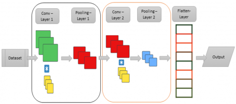
CNNs are designed to process and analyze visual data. This network excels at picture identification, categorization, and computer vision. CNNs are modeled after an animal's visual brain structure. The CNN’s system uses convolutional layers to independently and dynamically learn hierarchical patterns and attributes from input photos. Convolutional, pooling, and fully connected layers make up a CNN. Convolutional layers use filters to determine spatial hierarchies of attributes, whereas pooling layers minimize spatial dimensions and computational complexity. CNNs are a key technique in deep learning and excel in image-centric applications [39]. Furthermore, CNNs are popular for detecting deepfake videos. CNNs outperform and demonstrate superior scalability compared with other supervised learning approaches in AI for image and video processing. These CNNs can also extract image data for various applications.
In deepfake detection, the incorporation of additional supervised learning techniques can improve the model's accuracy and robustness. CNNs have input, output, and hidden layers, similar to standard neural networks. The deep layers convolutionally process first-layer inputs. In this context, convolution means matrix multiplication or dot product. CNNs use a nonlinearity activation function, such as the rectified linear unit (RELU), after matrix multiplication and then pool layers. Pooling layers calculate outputs using maximum or average pooling to minimize data dimensionality [40]. The main structure of these convolutional networks is illustrated in Figure 3.
Figure 3. Basic structure of CNNs [41, 42]
This section covers the specific methods utilized to carry out the research, involving multiple sequential phases, outlined as follows:
4.1 Preprocessing stage
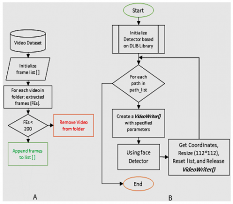
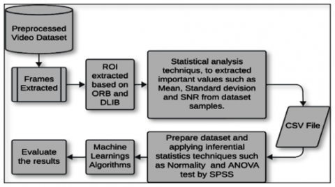
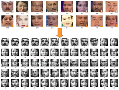
This part delineates the fundamental procedures used for creating the video dataset (FF++), which encompassed the preliminary processing of the samples. Figure 4(A) depicts a schematic illustrating the key processes involved in filtering out video clips that do not fulfill the frame number criterion of being fewer than 200. The objective is to obtain a more consistent distribution of video clips with an equal number of frames.
In the subsequent phase, a series of fundamental preprocessing procedures was conducted (Figure 4(B)). These procedures encompassed frame extraction and the identification of the facial region, which is deemed crucial in the context of the deep fake issue (specifically, face swapping). A widely acclaimed library in the domain of computer vision known as DLIB C++ [43] was utilized to accomplish this task. Furthermore, the tire size is standardized to fixed dimensions of 112×112. Finally, the frames are saved into a video clip file once more.
Figure 4. The preprocessing stage of our study is (A) dataset video filtering and (B) pretreatment procedures for sample preparation
4.2 Determine the most affected facial areas
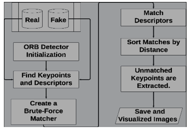
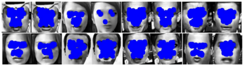
ORB is a computer vision and image processing feature descriptor. This algorithm is important for object recognition and matching because it detects and describes image key points. After capturing frames and preprocessing them via the preprocessing stage, the ORB method is applied to recognize critical spots and compute descriptors on each frame inside the real/fake class. The process is illustrated in Figure 5, providing a detailed explanation of each step. Consequently, a collection of unmatched key points and their corresponding descriptions is obtained.
The ORB algorithm steps in the diagram Figure 5 are as follows: Firstly, FAST finds corners by comparing pixel intensities in a circular pattern around a pixel. Secondly, the keypoint locations are refined by fitting a 2D quadratic function to pixel intensities surrounding each candidate keypoint. Thirdly, the aspects orient each key point to make the method rotation-invariant. Fourthly, BRIEF is used to create a binary feature descriptor for each key point. Our work uses brute-force matching to uncover the correspondences between the key points in the two frames. Finally, a classification is applied to keep only mismatched points. The Hamming distance for binary descriptors in ORB is often used as a distance metric threshold.
Figure 5. Outline the procedural steps of the ORB algorithm as employed in our work
4.3 Post-preprocessing
After identifying the most influential areas based on the approach in Section 4.2, we undertake systematic post-processing to accurately extract that area, which involves relying on the DLIB library to determine the key points and segment the influential area based on these points. Briefly, DLIB uses a pre-trained model to extract facial landmarks and generate a list of coordinates. Image and facial landmarks are fed to the segment face function. A binary mask is initialized with zero values to partition the face. The identification of landmarks helps remove comparable areas of the image and allocate them to the mask to determine facial regions. The frontal, ocular, nasal, oral, and buccal regions are included. The mask portrays the landmark-segmented face.
4.4 Apply different analysis methods
The objective of the analysis is to use inferential statistics to examine the behaviors of samples extracted from the dataset, which represents the target population for investigation. Inferential statistics are suitable for the deepfake problem because they provide trustworthy detection by explaining the discrepancies between deepfakes and real videos. A description of the population samples of the FF++ data set was utilized, which can effectively aid in identifying statistical significance and distinguishing between fake and real community samples.
The mean ($\mu$) and standard deviation (σ) values and $\sigma$ are calculated for each target sample in the genuine and false classes. The features in our study are the dependent variables we have chosen, whilst the title of the variety (real or fake) reflects the independent factors. An essential test in analytical research is to verify the nature of the data by examining its normal distribution. A normal distribution test is used to ascertain whether a dataset adheres to the anticipated pattern of a normal distribution, which is a prerequisite for performing subsequent statistical analysis with confidence.
The three ways to test the sample characteristics are as follows [44]: The skewness and kurtosis z-values should be −1.96 to +1.96. The Shapiro–Wilk p-value should be above 0.05. Histograms, normal Q–Q plots, and box plots should show our data’s roughly normal distribution. The data deviation is determined upon verification of the data distribution, indicating the extent of variation amongst the samples under examination. This notion can be confirmed by conducting a one-way ANOVA test with a p-value of less than 0.05.
Consequently, the null hypothesis is refuted, resulting in the acceptance of our alternative hypothesis. A t-test must also be tested to prove our alternative hypothesis that statistical differences exist between the real and the artificially generated samples of the two categories [45]. Figure 6 shows the main outline of the analysis methodology in this study.
Figure 6. Summary of our study’s analysis methodology
4.5 Similarity measurement analysis
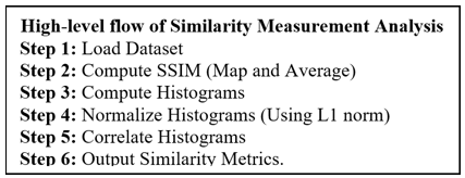
Measuring perceptual and statistical similarities between images involves utilizing the SSIM and correlation coefficient, which are examples of image similarity metrics [46] The local patterns of pixel intensities are compared using SSIM to show structural similarities. Visual consistency is indicated by correlation, which quantifies the strength of the linear relationship between pixel values in two images. Both metrics are helpful for diagnosing problems with images and providing similarity analysis based on global statistical dependencies and localized structural patterns in computer vision applications. The pseudocode can be observed in Figure 7, which shows the main steps involved in calculating the values of the two metrics used.
Figure 7. Investigation of the main SSIM and correlation methods
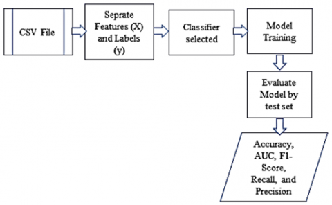
4.6 Implementing ML algorithms
Binary classification is a prevalent problem in supervised ML, where an algorithm is trained on labeled data and used to predict a discrete class label of either zero or one for fresh, unseen data. Multiple conventional ML techniques exhibit strong performance in binary classification tasks. The aforementioned techniques encompass logistic regression, decision trees, support vector machines, and neural networks. The choice of algorithm is contingent upon various aspects, such as the desired level of efficiency, precision, and comprehensibility for a certain task. In our current study, six of the most popular ML algorithms in computer vision are used [47]. The diagram in Figure 8 shows the most important steps followed to complete training one of the aforementioned classifiers and evaluate it.
Figure 8. Primary phases of ML algorithms
4.7 Proposing a CNN architecture
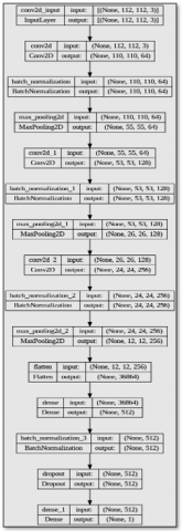
In this simple architecture of a deep convolutional network, which was proposed in our analytical study of deepfake sample generation behaviors, we incorporated preprocess and postprocess stages for the dataset used. Our CNN is structured with a sequential architecture consisting of three convolutional layers. After each convolutional layer, batch normalization and max pooling procedures are applied to extract hierarchical features from the input images. The model proceeds by incorporating a flattening layer to facilitate the subsequent fully connected layers, followed by a dense layer consisting of 512 neurons, activated using the RELU function. Batch normalization and dropout techniques are then applied to regularise the model. The output layer for binary classification consists of a final dense layer with a single neuron and sigmoid activation. The architecture of the convolutional network proposed in this study is depicted in Figure 9.
Figure 9. Customize CNN map created in our study
This section will focus on the key findings obtained during the study of this analytical investigation. The section encompasses a graphical representation of the main findings, together with the crucial values and inferences upon which they were founded. All the results were obtained from the FF++ dataset, which underwent preprocessing in our study to identify facial areas and other relevant factors, such as ROI, as explained in Section 5.3. Out of the total samples, 4940 were identified as fake frames, while 4916 were used as real samples. We also utilized evaluation tools and metrics to assess any methodology utilized in our study.
5.1 Evaluation metrics used
ML models are evaluated using a variety of performance criteria. The percentage of accurate forecasts out of all predictions provides a comprehensive measure of correctness. The F1-Score, which is the harmonic mean of precision and recall, provides a balance between true positives and false positives and negatives. This balance is beneficial in imbalanced class datasets. A greater area under the ROC curve (AUC) indicates improved model performance in distinguishing positive and negative samples. Recall, sometimes called sensitivity, measures the model’s capacity to detect all relevant instances, whereas precision measures positive predictions. The confusion matrix analyses true positives, true negatives, false positives, and false negatives to reveal a model’s categorization skills and limitations. These indicators provide a complete picture of an ML model’s ability to predict numerous performance factors [48, 49]. Table 3 briefly explains each measure.
Table 3. Summary of the key study evaluation measures [50]
|
Metrics |
Description |
Formula |
|
Accuracy |
Accuracy is a metric that quantifies the degree of correctness of a model. It computes the proportion of accurately anticipated cases out of the total instances. |
$Acc=\frac{Number\ of\ Correct\ Predictions}{Total\ Number\ of\ Predictions}$ |
|
Recall |
Recall, which is often referred to as sensitivity or true positive rate, quantifies the model’s capacity to accurately detect all pertinent events. |
$Recall=\frac{True\ Positives}{True\ Positives+False\ Negatives}$ |
|
Precision |
Precision quantifies the accuracy level of correctness in optimistic forecasts. It computes the proportion of accurately predicted positive observations out of all the projected positives. |
$Precision=\frac{True\ Positives}{True\ Positives+False\ Positives}$ |
|
F1-Score |
The F1-Score is calculated as the harmonic mean of precision and recall. It offers a tradeoff between precision and recall, which is especially beneficial in cases when the distribution of classes is imbalanced. |
$F1-Score=2 \times \frac{Precision \times Recall}{Precision+ Recall}$ |
|
Area under the ROC curve (AUC) |
AUC quantifies the extent of the area beneath the ROC curve. It denotes the model’s capacity to differentiate between positive and negative cases. |
The AUC is typically calculated using integration techniques on the ROC curve. |
5.2 Dataset used
FaceForensics++ (FF++) is a benchmark for deepfake detection techniques. This benchmark contains facial alteration videos, including deep learning-based ones. The dataset comprises a collection of authentic videos featuring humans engaging in speech or doing diverse actions, totaling 1000 video recordings. Deepfake videos are generated by altering the original videos’ faces. These changes involve replacing the face of the video’s subject with a deep learning-generated one. This section contains 5000 changed samples [50]. This dataset can be considered one of the most important and extensive datasets in the deepfake problem.
Moreover, this dataset summarises the biggest obstacles, including lighting, positions, and facial expressions, to recreate real-world events and incorporates a diverse range of deepfake creation methods to test detection algorithms. Besides, The FF++ data set's challenges are quality (the dataset includes manipulated videos at different compression levels), a manipulation technique (Deepfakes, Face2Face, Face Swap, and NeuralTextures), and source (YouTube, which may introduce biases in content demographics, and recording conditions) [51]. Preprocessing the data set to filter it solved these problems. Plus, it will analyze model performance across quality levels, the robustness of compression artifacts, and augment the dataset.
5.3 Pre/post-process output
Figure 10 shows some of the results obtained after applying the approach in Section 4.1 to perform the initial processing. Figure 11 shows some of the results obtained using the ORB algorithm to identify the region of interest after conducting the methodology used in Section 4.2. Finally, Figure 12 shows the results obtained after conducting the post-processing approach referred to in Section 4.3.
Figure 10. Preprocessing stages in our study
Figure 11. Identify the area of interest
Figure 12. DLIB library used to isolate the impacted facial regions
5.4 Statistical tests
Statistical tests are conducted to compare the two classes. The t-statistic (t-value) and p-value are commonly used statistical methods for testing population samples. The t-statistic and p-value derived from a t-test are crucial elements utilized to draw conclusions about the population based on the sample data [52, 53]. Table 4 briefly explains these concepts with the mathematical formula for each.
Table 4. Three common measures utilized in statistical analysis
|
Statistical Tests |
Description |
Formula |
|
T-statistic (t-value) |
The t-statistic measures the difference between the sample average and the estimated population average, taking into consideration the sample mean’s standard deviation. |
$\frac{\overline{X_1}-\overline{X_2}}{\sqrt{\frac{s_1^2}{n_1}+\frac{s_2^2}{n_2}}}$ and $\overline{X_1}-\overline{X_2}$ are the sample means of the two groups, $s_1$ and $s_2$ are the sample standard deviations of the two groups, and $n_1$ and $n_2$ are the sample sizes of the two groups. |
|
p-value |
The p-value is the probability of seeing a t-statistic as extreme as or more extreme than the sample data one if the null hypothesis is valid. A small p-value (typically less than 0.05) suggests that you can reject the null hypothesis. |
The p-value formula depends on the t-test and assumptions. In the two-sample t-test, the CDF of the t-distribution is used. General form: $p=P(|T|>|t|)$, where, $T$ is a random variable from the t-distribution, whilst $t$ is the observed t-statistic. |
|
Levene's test [54] |
A Levene’s test is used to assess the equality of variances for a variable calculated for two or more groups. A significant Levene’s result means proceeding with caution or using alternate analyses that do not assume equal variances. |
$W=\frac{(N-k)}{(k-1)} \cdot \frac{\sum_{i=1}^k N_i\left(Z_{i .}-Z_{. .}\right)^2}{\sum_{i=1}^k \sum_{j=1}^{N_i}\left(Z_{i j}-Z_{i .}\right)^2}$, where, $k$ is the number of different classes to which category the sampled cases belong, $N_i$ is the number of cases in the $i$ classes, $N$ is the total number of cases in all classes, and $Y_{i j}$ is the value of the measured variable for the $j$ th case of the $i$ classes. Whilst $Z_{i j}= \begin{cases}\left|Y_{i j}-\bar{Y}_{i .}\right|, & \bar{Y}_i . \text { is a mean of the } i \text {-th group } \\ \left|Y_{i j}-\tilde{Y}_i\right|, & \tilde{Y}_i . \text { is a median of the } i \text {-the group. }\end{cases}$ |
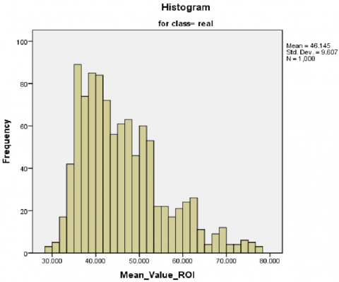
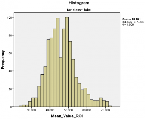
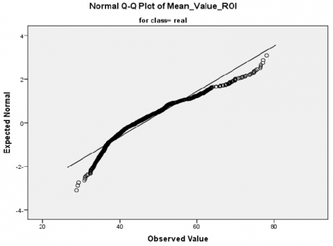
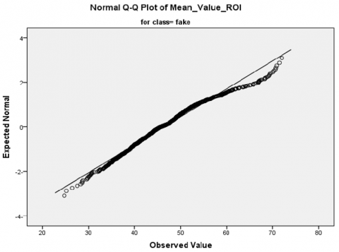
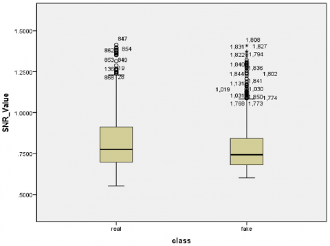
Firstly, a normally distributed test applies to our dataset, utilizing a Shapiro–Wilk test (p-value < 0.05) for each value feature extracted (mean, standard, and SNR values) [53]. Specifically, the low Shapiro–Wilk p-values and statistics indicate that the real and fake class sample data do not conform to a normal distribution according to this test. Secondly, visual inspection of the histogram, normal Q–Q plots, and box plots for all scalar values showed that our dataset is not normally distributed for real and fake classes (Figures 13 and 14, respectively). Finally, skewness and kurtosis are computed for each class of mean, standard, and SNR (Table 5). Consequently, we refute the null hypothesis that the data exhibit a normal distribution based on the outcomes of the three aforementioned tests. Appendix A provides the additional results.
Figure 13. Histogram, normal Q–Q plots of mean feature values in our study
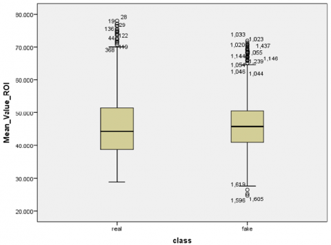
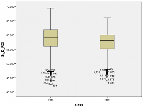
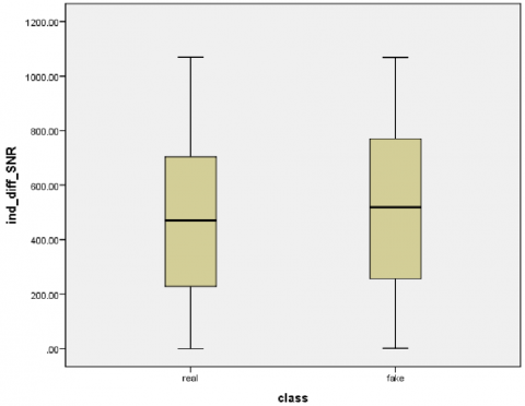
Figure 14. Box plots of the mean, standard, and SNR for each class
Table 5. Skewness and kurtosis p-values for each class
|
Dependent Variables |
Class |
Skewness |
Kurtosis |
|
SNR |
Real |
1.326 (SE: 0.077) |
1.574 (SE: 0.155) |
|
Fake |
1.454 (SE: 0.077) |
1.595 (SE: 0.155) |
|
|
Mean |
Real |
0.905 (SE: 0.077) |
0.425 (SE: 0.155) |
|
Fake |
0.520 (SE: 0.077) |
0.560 (SE: 0.155) |
|
|
Standard dev. |
Real |
−0.934 (SE: 0.077) |
0.544 (SE: 0.155) |
|
Fake |
−0.816 (SE: 0.077) |
0.061 (SE: 0.155) |
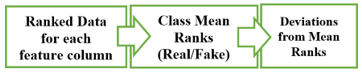
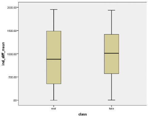
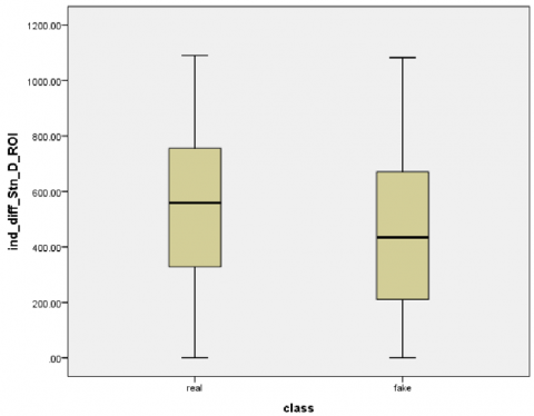
In this case, non-parametric methods for subsequent variance testing will be used because they make no assumptions about the distributions. Accordingly, the non-parametric Levene test should be performed. Preprocessing must be carried out to prepare the data for subsequent tests. Preprocessing encompasses the stages depicted in the diagram in Figure 15. After preparing the data, it can be displayed as in the box plots in Figure 16, where the stability of the data can be observed, and the outliers are eliminated. All results and graphics can be found in Appendix A.
Given that our analyzed data do not exhibit a tendency towards a normal distribution when subjected to testing, it can be deemed non-parametric. Accordingly, a test will be conducted using Levene’s test for non-normally distributed data [55]. However, this examination is conducted after the data is prepared in accordance with the procedures outlined in the chart in Figure 15. We will then analyze these individual differences using an ANOVA.
Figure 15. Initial data preparation steps in our study
Figure 16. Mean, standard, and SNR box plots from the left to right after the preparation steps
The null hypothesis states that variance is equal. The null hypothesis and equality of variance are maintained if the p-value surpasses 0.05. If the p-value is less than 0.05, then we can reject the null hypothesis and infer that the two categories statistically differ in variance or spread [56]. Table 6 shows the p-values obtained for each column with features of the dependent values for the mean, standard deviation, and SNR values.
The values obtained after performing the ANOVA test analysis to examine the equality of variance are less than 0.05, indicating that the null hypothesis failed. This result indicates that a statistically significant difference in the variances exists between the classes at the 0.05 significance level.
The results obtained according to the above-mentioned two measures were as follows: the t-statistics were approximately 0.122, 0.132, and 0.020 for the mean, standard, and SNR values, respectively. Given the unequal variances for the mean and standard deviation, no significant difference exists in the means between the two groups (p>0.05). However, a statistically significant difference exists between classes at the p<0.05 level of the SNR variable. The small p-value of SNR allows us to reject the idea that no difference exists (reject the null hypothesis.). Thus, our results support the alternative hypothesis that a true difference exists between the dataset of the two independent classes, real and fake. Table 7 shows the results obtained based on the SPSS test.
Table 6. Results were obtained based on a one-way ANOVA
|
Dependent Variable |
p-value (sig) |
|
Mean |
0.005 |
|
Standard deviation |
0.000 |
|
SNR |
0.005 |
Table 7. Mean, standard, and SNR p-values based on t-test measures
|
Independent Samples Test |
||||
|
t-Test for Equality of Means |
||||
|
t |
Sig. (2-Tailed) |
Mean Difference |
Std. Error Difference |
|
|
St. deviation |
-1.511 |
0.131 |
-37.00823 |
24.49794 |
|
-1.511 |
0.131 |
-37.00823 |
24.48604 |
|
|
SNR |
2.323 |
0.020 |
56.61338 |
24.36903 |
|
2.322 |
0.020 |
56.61338 |
24.37712 |
|
|
Mean |
0.122 |
0.903 |
2.98264 |
24.37234 |
|
0.122 |
0.903 |
2.98264 |
24.37206 |
|
5.5 Analysis based on similarity measurement
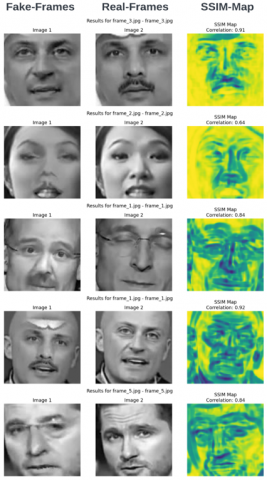
Similarity measures evaluate the similarity of a pair of images, quantifying similarity, visual similarities, and contrasts between images. The SSIM and correlation coefficient are widely used image similarity measures that gauge the perceptual and statistical similarities of images in complimentary manners. SSIM and correlation are used together to analyze the similarity of images. These measures assess the localized structural patterns and the global statistical dependencies to measure visually perceptible differences and perceptually correlated appearances between pairs of images. The methodology of these measures provides a strong and adaptable method for evaluating image quality and diagnosing issues in various computer vision applications. The samples for this study were carefully selected to carry out this test. After the GAN algorithm processed the clips, 100 genuine videos and an equal number of false videos were obtained. A portion of the results is graphically displayed in Figure 17, and some calculated values are also visible in Table 8.
Figure 17. The structural similarity index measure map
Table 8. Some results of the SSIM and correlation scalers from our study analysis
|
Image Pair |
SSIM |
Correlation |
|
1 |
0.698225 |
0.902769603 |
|
2 |
0.70416 |
0.905171778 |
|
3 |
0.706193 |
0.908827302 |
|
4 |
0.325047 |
0.907112308 |
|
5 |
0.694204 |
0.910736524 |
|
6 |
0.717101 |
0.626169936 |
|
7 |
0.718841 |
0.638290493 |
|
8 |
0.716083 |
0.617257874 |
|
9 |
0.285033 |
0.489076281 |
|
10 |
0.282202 |
0.477282469 |
|
11 |
0.330275 |
0.842049054 |
|
12 |
0.332535 |
0.856355891 |
|
13 |
0.323593 |
0.857792007 |
|
14 |
0.318422 |
0.860929033 |
|
15 |
0.318707 |
0.864377332 |
The analysis of the results of the structural similarity (SSIM) and correlation values of the image frame pairs in the dataset demonstrates visible disparities between frames within each class. However, the frames still portray content that is strongly associated. Specifically, the SSIM values, which are typically moderate and fall within the range of 0.2 to 0.8, suggest clear differences in the pixel and structural characteristics across the pairs of frames when compared directly. Nevertheless, correlation coefficients above 0.8 indicate a significant linear relationship and visual similarity between the frame contents, specifically in terms of the overall visual structure and semantics. This result indicates that although the frames may exhibit local variations, which are likely caused by certain factors, such as noise, artifacts, and lighting, resulting in a decrease in the structural similarity index (SSIM), the overall appearance and substance of the image remain consistent, as evidenced by the maintained correlation.
In summary, the metrics measure the differences in quality and exact appearance that are evident inside a specific frame but are mathematically identical across other frames.
5.6 Machine learning classifiers test
In this section, the retrieved features are examined after undergoing preparation in Figure 15, which are used in the data preparation, and their values are saved in a CSV file to be inputted into the ML methods used in our study, as depicted in Figure 8. Consequently, the results shown in Table 9 are obtained.
According to the data in Table 8, the Bagging classifier is the top-performing model overall, with an accuracy of 0.7125 and an F1 score of 0.7132. This feature makes this model the most precise for accurately guessing the binary classification labels. The majority of the models exhibit accuracy ratings ranging from the upper 60 s to the lower 70 s. The SVM and decision tree models had the lowest performance, with an accuracy below 0.67. In conclusion, the metrics demonstrate that our models have achieved a moderate level of performance in the binary classification on this dataset. A multitude of practical applications could benefit from models that possess an accuracy rate of approximately 70%. However, additional optimization may be necessary to enhance accuracy, F1 score, and other relevant metrics, depending on the specific requirements of the use case. Overall, these initial results are fairly satisfactory. Nonetheless, a higher level of accuracy is imperative in detecting deepfakes. This necessity prompts us to create a deep convolutional network to accomplish the task of extracting patterns from the dataset that was preprocessed in our study.
Table 9. Results of the ML algorithm evaluation based on metrics
|
ML_Classifier |
Accuracy |
F1 Score |
AUC |
Precision |
Recall |
|
Gaussian process |
0.6825 |
0.684863524 |
0.682479562 |
0.683168317 |
0.686567164 |
|
Bagging classifier |
0.7225 |
0.725925926 |
0.722455561 |
0.720588235 |
0.731343284 |
|
SVM |
0.6725 |
0.679706601 |
0.67240431 |
0.668269231 |
0.691542289 |
|
RF |
0.6925 |
0.700729927 |
0.692379809 |
0.685714286 |
0.71641791 |
|
Decision tree |
0.66 |
0.656565657 |
0.660066502 |
0.666666667 |
0.646766169 |
|
KNN |
0.6975 |
0.704156479 |
0.697404935 |
0.692307692 |
0.71641791 |
|
XGBoost |
0.68 |
0.689320388 |
0.679866997 |
0.672985782 |
0.706467662 |
|
LightGBM |
0.7125 |
0.713216958 |
0.712505313 |
0.715 |
0.711442786 |
5.7 Custom CNN test
The CNN described in Section 4.7, as shown in Figure 9, has undergone training. We utilize the dataset containing the extracted region of interest to train our neural network. After fine-tuning the hyper-parameters of our suggested model, we determined the optimal settings through a combination of experience and effort. Table 10 shows in detail the configuration of our proposed convolutional neural network, which includes three convolutional layers and two dense layers. At the same time, the specific hyper-parameter values used in our study can be found in Table 11, which provides a comprehensive overview of our adopted settings.
Table 10. The architecture of proposed CNN
|
Layer |
Output Shape |
Parameters |
|
Conv 2D - 1 |
(None, 110, 110, 64) |
640 |
|
Batch normalization -1 |
(None, 110, 110, 64) |
256 |
|
Max Pooling 2D -1 |
(None, 55, 55, 64) |
0 |
|
Conv 2D - 2 |
(None, 53, 53, 128) |
73856 |
|
Batch normalization -2 |
(None, 53, 53, 128) |
512 |
|
Max Pooling 2D -2 |
(None, 26, 26, 128) |
0 |
|
Conv 2D - 3 |
(None, 24, 24, 256) |
295168 |
|
Batch normalization -3 |
(None, 24, 24, 256) |
1024 |
|
Max Pooling 2D -3 |
(None, 12, 12, 256) |
0 |
|
Flatten -1 |
(None, 36864) |
0 |
|
Dense 1 |
(None, 512) |
18874880 |
|
Batch normalization -4 |
(None, 512) |
2048 |
|
Dropout |
(None, 512) |
0 |
|
Dense 2 |
(None, 1) |
513 |
Table 11. Hyperparameters and augmentation settings are used in our customized CNN
|
Hyperparameter |
Value |
|
Frame size |
112×112 |
|
Number of train set |
2411 |
|
Number of test set |
603 |
|
Loss function |
Binary cross-entropy |
|
Conv-activation function |
RELU |
|
Min-learning rate |
1e-6 |
|
Optimizer |
Adam |
|
Batch sizes |
32 |
|
Epochs |
100 |
|
Augmentation settings [57] |
|
|
Rotation range |
15 |
|
(Width and height) shift range |
0.1 |
|
(Shear and zoom) range |
0.1 |
|
Fill mode |
Nearest |
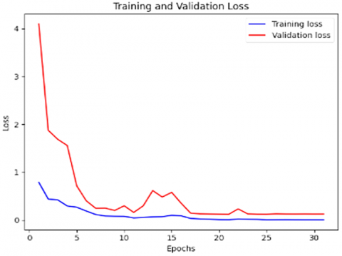
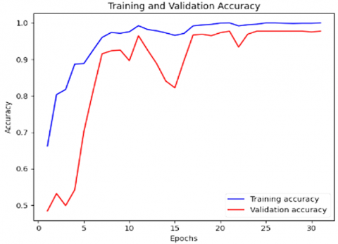
Table 12 displays the performance measurements for each class and the final evaluation results of the model. The effectiveness of our proposed model, which utilizes a simple CNN, is demonstrated by comparing it to previous ML models. This result is evident from the accuracy and loss visualizations shown in Figure 18, highlighting the model’s efficiency. The model incorporates regularisation techniques for deep neural networks to mitigate the issue of overfitting [58]. Table 13 explains the superiority of our proposed model over some related studies because we obtained an accuracy of 97% percent when testing the model on the dataset FF++.
Figure 18. Loss and accuracy plots of the proposed model
Table 12. Classification report of our CNN model
|
Class |
Precision |
Recall |
F1 Score |
Support |
|
Real |
0.98 |
0.96 |
0.97 |
320 |
|
Fake |
0.96 |
0.98 |
0.97 |
283 |
|
Accuracy |
0.97 |
603 |
||
|
Macro avg |
0.97 |
0.97 |
0.97 |
603 |
Table 13. Comparing our proposed model with some related work
|
Reference |
Dataset |
Accuracy (%) |
AUC (%) |
|
[60] |
FF++ |
85.84 |
72.17 |
|
[61] |
90.72 |
95.26 |
|
|
[62] |
81.33 |
77.01 |
|
|
[63] |
80.03 |
77.71 |
|
|
[64] |
82.99 |
- |
|
|
Our model |
97 |
91.54 |
Figure 18 shows the stability of the proposed model at a learning rate of 0.00004 after 27 epochs. Moreover, it can be noted that the problem of overfitting and underfitting has been eliminated in our proposed structure. The AUC is applicable since it summarizes the model's class discrimination across all thresholds in a single value. The AUC for our deepfake detection model is calculated to improve the reliability of our findings. We compute the AUC and evaluate our model using sci-kit-learn's "roc_auc_score" function [59]. The model scores 0.9154 on the test dataset.
5.8 Challenges and limitations
One of the main challenges encountered during the investigation was the scarcity of widely certified standard resources. This dearth potentially constrained the capacity for some analyses because the initial processing and feature extraction procedures were conducted on a dataset comprising video data. On the other hand, there are several limitations:
Firstly, statistical tests like t-tests, ANOVA, and correlation analyses assume a normal distribution. However, non-normal data can lead to increased Type I error rates, reduced statistical power, and biased estimates [65]. Small sample sizes or skewed data can increase the probability of rejecting the null hypothesis. To mitigate these issues, we are using data transformations, such as the initial preparation steps in Figure 15, and use non-parametric tests that do not rely on the normality assumption, such as Levene’s test.
Secondly, one of the limitations of this study is that it was carried out using only one dataset, specifically the FF++ dataset. However, the investigation did not encompass the evaluation of imperceptible samples.
5.9 Recommendations
A set of recommendations can be concluded based on our study as follows:
• Thorough examination of the behavior of deepfake content-generating algorithms and methodologies can aid in developing practical solutions for future detection methods.
• Expanding the scope of diverse statistical analytic techniques, such as exploratory data analysis (EDA) and statistical modeling, might significantly aid researchers in identifying deep fakes concealed inside multimedia content.
• Studying the structure of examples by investigating correlations and similarities like the Spearman correlation. Likewise, assessing different forms of distortions using measures such as the Peak Signal to Noise Ratio (P-SNR) and Visual Signal to Noise Ratio (V-SNR) leads to positive results.
• Media authenticity is verified throughout its life cycle using watermarking, media verification markers, and chain-of-custody logging.
In conclusion, a comprehensive and diverse approach must be utilized to protect the truth and ensure freedom of expression. Any countermeasure must have a dual purpose to mitigate the adverse societal consequences of harmful deep-fake technology. The first objective is to address the exposure to malicious deepfakes, whilst the second one is to limit the potential harm that they can cause. Apart from authentication and provenance, all deepfake detection countermeasures focus on short-term solutions. Accordingly, inferential statistical methods can help address complex challenges like deepfakes by drawing meaningful and reasonable conclusions about the population under study.
Deepfake detection lacks extensive analysis methods to uncover significant features that could address generalization in this domain. As well as this study uses statistical methods and similarity measurements, making it unique. This could aid future research into this topic and help uncover deep fakes in multimedia content. Rejecting the null theory showed statistically significant differences supporting the alternative hypothesis. Where about 1,400 FF++ videos were analyzed; moreover, a proposed preprocessing strategy identified the most influential locations for conditional generative adversarial networks.
As part of future work, the study of deepfakes reveals a similarity to discovering vulnerabilities in computer systems and anti-programs (filling gaps). Accordingly, continuous updating is essential because deepfake contents change according to detection models. In the future, it may be feasible to analyze the generated samples created using generative adversarial algorithms systematically. This analysis can involve more advanced methods, such as examining the signal frequencies of these samples and comparing them to the frequencies of real samples. Alternatively, sophisticated techniques in digital signal processing can be used to differentiate between deep false samples and authentic samples. From another viewpoint, a comprehensive future solution is needed. Adding security algorithms (such as a hash algorithm) to digital capture devices (such as a webcam) gives each real clip a unique identifier that the corresponding verification algorithms can easily verify. Specifically, security software embedded in digital content capture devices can contribute to a final solution to this problem.
[1] Akhtar, Z. (2023). Deepfakes generation and detection: A short survey. Journal of Imaging, 9(1): 18. https://doi.org/10.3390/jimaging9010018
[2] Saxena, D., Cao, J. (2021). Generative adversarial networks (GANs) challenges, solutions, and future directions. ACM Computing Surveys (CSUR), 54(3): 1-42. https://doi.org/10.1145/3446374
[3] Aneja, S., Midoglu, C., Dang-Nguyen, D.T., Khan, S.A., Riegler, M., Halvorsen, P., Bregler, C., Adsumilli, B. (2022). ACM multimedia grand challenge on detecting cheapfakes. ArXiv: 2207.14534. https://doi.org/10.48550/arXiv.2207.14534
[4] Buo, S.A. (2020). The emerging threats of deepfake attacks and countermeasures. ArXiv: 2012.07989. https://doi.org/10.48550/arXiv.2012.07989
[5] Patel, Y., Tanwar, S., Gupta, R., Bhattacharya, P., Davidson, I.E., Nyameko, R., Aluvala, S., Vimal, V. (2023). Deepfake generation and detection: Case study and challenges. IEEE Access, 11: 143296-143323. https://doi.org/10.1109/ACCESS.2023.3342107
[6] Masood, M., Nawaz, M., Malik, K.M., Javed, A., Irtaza, A., Malik, H. (2023). Deepfakes generation and detection: State-of-the-art, open challenges, countermeasures, and way forward. Applied Intelligence, 53(4): 3974-4026. https://doi.org/10.1007/s10489-022-03766-z
[7] Salvatore, D. (2021). Theory and Problems of Statistics and Econometrics. Mcgraw-Hill, USA. https://doi.org/10.1036/0071395687
[8] St, L., Wold, S. (1989). Analysis of variance (ANOVA). Chemometrics and Intelligent Laboratory Systems, 6(4): 259-272. https://doi.org/10.1016/0169-7439(89)80095-4
[9] Cha, S.H. (2007). Comprehensive survey on distance/similarity measures between probability density functions. City, 4(1): 300-307. https://pdodds.w3.uvm.edu/research/papers/others/everything/cha2007a.pdf.
[10] Sokoliuk, A., Kondratenko, G., Sidenko, I., Kondratenko, Y., Khomchenko, A., Atamanyuk, I. (2020). Machine learning algorithms for binary classification of liver disease. In 2020 IEEE International Conference on Problems of Infocommunications. Science and Technology (PIC S&T), Kharkiv, Ukraine, pp. 417-421. https://doi.org/10.1109/PICST51311.2020.9468051
[11] Hashim, A.N., Jassim, M.F., Hashim, A.T. (2023). Storage space reduction of biometric iris databases by successive images differences and quadtree decomposition. Mathematical Modelling of Engineering Problems, 10(5): 1683-1689. https://doi.org/10.18280/mmep.100518
[12] Shad, H.S., Rizvee, M.M., Roza, N.T., Hoq, S.A., Monirujjaman Khan, M., Singh, A., Singh, A., Zaguia, A., Bourouis, S. (2021). Comparative analysis of deepfake image detection method using convolutional neural network. Computational Intelligence and Neuroscience, 2021(1): 3111676. https://doi.org/10.1155/2021/3111676
[13] Le, B., Tariq, S., Abuadbba, A., Moore, K., Woo, S. (2023). Why do deepfake detectors fail. arXiv: 2302.13156. https://doi.org/10.1145/3595353.3595882
[14] Li, Y. (2018). Exposing deepfake videos by detecting face warping artif acts. arXiv: 1811.00656. https://doi.org/10.48550/arXiv.1811.00656
[15] Marra, F., Gragnaniello, D., Verdoliva, L., Poggi, G. (2019). Do gans leave artificial fingerprints? In 2019 IEEE conference on multimedia information processing and retrieval (MIPR), San Jose, USA, pp. 506-511. https://doi.org/10.1109/MIPR.2019.00103
[16] Gragnaniello, D., Cozzolino, D., Marra, F., Poggi, G., Verdoliva, L. (2021). Are GAN generated images easy to detect? A critical analysis of the state-of-the-art. In 2021 IEEE International Conference on Multimedia and Expo (ICME), Shenzhen, China, pp. 1-6. https://doi.org/10.1109/ICME51207.2021.9428429
[17] Guarnera, L., Giudice, O., Battiato, S. (2020). Deepfake detection by analyzing convolutional traces. In Proceedings of the IEEE/CVF Conference on Computer Vision and Pattern Recognition Workshops, Seattle, USA, pp. 666-667. https://doi.org/10.1109/CVPRW50498.2020.00341
[18] Giudice, O., Guarnera, L., Battiato, S. (2021). Fighting deepfakes by detecting GAN DCT anomalies. Journal of Imaging, 7(8): 128. https://doi.org/10.3390/jimaging7080128
[19] Dong, S.C., Wang, J., Ji, R.H., Liang, J.J., Fan, H.Q., Ge, Z. (2023). Implicit identity leakage: The stumbling block to improving deepfake detection generalization. In Proceedings of the IEEE/CVF Conference on Computer Vision and Pattern Recognition, Vancouver, Canada, pp. 3994-4004. https://doi.org/10.1109/CVPR52729.2023.00389
[20] Mitra, A., Mohanty, S.P., Corcoran, P., Kougianos, E. (2021). A machine learning based approach for deepfake detection in social media through key video frame extraction. SN Computer Science, 2(2): 98. https://doi.org/10.1007/s42979-021-00495-x
[21] Wodajo, D., Atnafu, S. (2021). Deepfake video detection using convolutional vision transformer. arXiv: 2102.11126. https://doi.org/10.48550/arXiv.2102.11126
[22] Cao, Y.H., Li, S.Y., Liu, Y.X., Yan, Z.L., Dai, Y.T., Yu, P.S., Sun, L.C. (2023). A comprehensive survey of ai-generated content (AIGC): A history of generative AI from GAN to ChatGPT. arXiv: 2303.04226. https://doi.org/10.48550/arXiv.2303.04226
[23] Sontakke, N., Utekar, S., Rastogi, S., Sonawane, S. (2023). Comparative analysis of deep-fake algorithms. arXiv: 2309.03295. https://doi.org/10.48550/arXiv.2309.03295
[24] Mirza, M. (2014). Conditional generative adversarial nets. arXiv: 1411.1784. https://doi.org/10.48550/arXiv.1411.1784
[25] Douzas, G., Bacao, F. (2018). Effective data generation for imbalanced learning using conditional generative adversarial networks. Expert Systems with Applications, 91: 464-471. https://doi.org/10.1016/j.eswa.2017.09.030
[26] Rublee, E., Rabaud, V., Konolige, K., Bradski, G. (2011). ORB: An efficient alternative to SIFT or SURF. In 2011 International Conference on Computer Vision, Barcelona, Spain, pp. 2564-2571. https://doi.org/10.1109/ICCV.2011.6126544
[27] Imsaengsuk, T., Pumrin, S. (2021). Feature detection and description based on orb algorithm for FPGA-based image processing. In 2021 9th International Electrical Engineering Congress (iEECON), Pattaya, Thailand, pp. 420-423. https://doi.org/10.1109/iEECON51072.2021.9440232
[28] Grandini, M., Bagli, E., Visani, G. (2020). Metrics for multi-class classification: An overview. arXiv: 2008.05756. https://doi.org/10.48550/arXiv.2008.05756
[29] Orozco-Arias, S., Piña, J.S., Tabares-Soto, R., Castillo-Ossa, L.F., Guyot, R., Isaza, G. (2020). Measuring performance metrics of machine learning algorithms for detecting and classifying transposable elements. Processes, 8(6): 638. https://doi.org/10.3390/pr8060638
[30] Hore, A., Ziou, D. (2010). Image quality metrics: PSNR vs. SSIM. In 2010 20th International Conference on Pattern Recognition, Istanbul, Turkey, pp. 2366-2369. https://doi.org/10.1109/ICPR.2010.579
[31] Solaiyappan, S., Wen, Y. (2022). Machine learning based medical image deepfake detection: A comparative study. Machine Learning with Applications, 8: 100298. https://doi.org/10.1016/j.mlwa.2022.100298
[32] Cristianini, N. (2000). An Introduction to support Vector Machines and Other Kernel-Based Learning Methods. Cambridge University Press, UK. https://doi.org/10.1017/CBO9780511801389
[33] Breiman, L. (2001). Random forests. Machine Learning, 45: 5-32. https://doi.org/10.1023/A:1010933404324
[34] Joshi, A.V. (2022). Decision trees. In Machine Learning and Artificial Intelligence. Springer International Publishing, USA, pp. 73-87. https://doi.org/10.1007/978-3-031-12282-8_7
[35] Bishop, C.M. (2006). Pattern Recognition and Machine Learning by Christopher M. Bishop. Springer Science+ Business Media, New York, USA, pp. 78. https://link.springer.com/book/10.1007/978-0-387-45528-0.
[36] Yoon, H.I., Lee, H., Yang, J.S., Choi, J.H., Jung, D.H., Park, Y.J., Kim, S.M., Park, S.H. (2023). Predicting models for plant metabolites based on PLSR, AdaBoost, XGBoost, and LightGBM algorithms using hyperspectral imaging of Brassica juncea. Agriculture, 13(8): 1477. https://doi.org/10.3390/agriculture13081477
[37] Xiao, G.N., Cheng, Q., Zhang, C.Q. (2019). Detecting travel modes using rule-based classification system and Gaussian process classifier. IEEE Access, 7: 116741-116752. https://doi.org/10.1109/ACCESS.2019.2936443
[38] Jafarzadeh, H., Mahdianpari, M., Gill, E., Mohammadimanesh, F., Homayouni, S. (2021). Bagging and boosting ensemble classifiers for classification of multispectral, hyperspectral and PolSAR data: A comparative evaluation. Remote Sensing, 13(21): 4405. https://doi.org/10.3390/rs13214405
[39] O'Shea, K., Nash, R. (2015). An introduction to convolutional neural networks. arXiv: 1511.08458. https://doi.org/10.48550/arXiv.1511.08458
[40] Nguyen, T.T., Nguyen, Q.V.H., Nguyen, D.T., Nguyen, D.T., Huynh-The, T., Nahavandi, S., Nguyen, T.T., Pham, Q.V., Nguyen, C.M. (2022). Deep learning for deepfakes creation and detection: A survey. Computer Vision and Image Understanding, 223: 103525. https://doi.org/10.1016/j.cviu.2022.103525
[41] Kumar, A. (2022). Different types of CNN architectures explained: Examples. Vitalflux. https://vitalflux.com/different-types-of-cnn-architectures-explained-examples/.
[42] Shiri, F.M., Perumal, T., Mustapha, N., Mohamed, R. (2023). A comprehensive overview and comparative analysis on deep learning models: CNN, RNN, LSTM, GRU. arXiv: 2305.17473. https://doi.org/10.48550/arXiv.2305.17473
[43] King, D.E. (2009). DLIB-ML: A machine learning toolkit. The Journal of Machine Learning Research, 10: 1755-1758. https://www.jmlr.org/papers/volume10/king09a/king09a.pdf.
[44] Mitra, A.K. (2023). A step-by-step guide to data analysis using SPSS: Iron study data. Statistical Approaches for Epidemiology: From Concept to Application. Springer International Publishing, USA, pp. 343-362. https://doi.org/10.1007/978-3-031-41784-9_20
[45] Uhm, T., Yi, S. (2023). A comparison of normality testing methods by empirical power and distribution of p-values. Communications in Statistics-Simulation and Computation, 52(9): 4445-4458. https://doi.org/10.1080/03610918.2021.1963450
[46] Liu, C. (2014). Discriminant analysis and similarity measure. Pattern Recognition, 47(1): 359-367. https://doi.org/10.1016/j.patcog.2013.06.023
[47] Sen, P.C., Hajra, M., Ghosh, M. (2020). Supervised classification algorithms in machine learning: A survey and review. Emerging Technology in Modelling and Graphics: Proceedings of IEM Graph 2018, Springer Singapore, pp. 99-111.
[48] Domingos, P. (2012). A few useful things to know about machine learning. Communications of the ACM, 55(10): 78-87. https://doi.org/10.1145/2347736.2347755
[49] Géron, A. (2022). Hands-on Machine Learning with Scikit-Learn, Keras, and TensorFlow. O'Reilly, USA. https://cir.nii.ac.jp/crid/1130000797847732480.
[50] Rossler, A., Cozzolino, D., Verdoliva, L., Riess, C., Thies, J., Nießner, M. (2019). Faceforensics++: Learning to detect manipulated facial images. In Proceedings of the IEEE/CVF International Conference on Computer Vision, Seoul, Korea (South), pp. 1-11. https://doi.org/10.1109/ICCV.2019.00009
[51] Wang, J., Du, X.Y., Cheng, Y., Sun, Y.L., Tang, J.H. (2023). SI-Net: Spatial interaction network for deepfake detection. Multimedia Systems, 29(5): 3139-3150. https://doi.org/10.1007/s00530-023-01114-w
[52] Tzenios, N. (2023). Statistical Analysis in Research. Cambridge Open Engage. https://doi.org/10.33774/coe-2023-k71h2
[53] Shapiro, S.S., Wilk, M.B. (1965). An analysis of variance test for normality (complete samples). Biometrika, 52(3-4): 591-611. https://doi.org/10.1093/biomet/52.3-4.591
[54] Wooluru, Y., Swamy, D.R., Nagesh, P. (2016). Process capability estimation for non-normally distributed data using robust methods-a comparative study. International Journal for Quality Research, 10(2): 407. https://doi.org/10.18421/IJQR10.02-11
[55] Utama, E.P., Sudarsana, I.K. (2023). Effectiveness of treffinger model implementation to improving mathematics learning outcomes. International Journal of Multidisciplinary Sciences, 1(2): 232-240. https://doi.org/10.37329/ijms.v1i2.2369
[56] Nordstokke, D.W., Zumbo, B.D. (2010). A new nonparametric Levene test for equal variances. Psicológica, 31(2): 401-430. https://psycnet.apa.org/record/2011-19444-011.
[57] Wang, J., Perez, L. (2017). The effectiveness of data augmentation in image classification using deep learning. https://www.academia.edu/35482285.
[58] Bejani, M.M., Ghatee, M. (2021). A systematic review on overfitting control in shallow and deep neural networks. Artificial Intelligence Review, 54(8): 6391-6438. https://doi.org/10.1007/s10462-021-09975-1
[59] Pedregosa, F., Varoquaux, G., Gramfort, A., Michel, V., Thirion, B., et al. (2011). Scikit-learn: Machine learning in Python. Journal of Machine Learning Research, 12: 2825-2830.
[60] Suratkar, S., Kazi, F. (2023). Deep fake video detection using transfer learning approach. Arabian Journal for Science and Engineering, 48(8): 9727-9737. https://doi.org/10.1007/s13369-022-07321-3
[61] Cao, J.Y., Ma, C., Yao, T.P., Chen, S., Ding, S.H., Yang, X.K. (2022). End-to-end reconstruction-classification learning for face forgery detection. In Proceedings of the IEEE/CVF Conference on Computer Vision and Pattern Recognition, New Orleans, USA, pp. 4113-4122. https://doi.org/10.1109/CVPR52688.2022.00408
[62] Dong, S.C., Wang, J., Liang, J.J., Fan, H.Q., Ji, R.H. (2022). Explaining deepfake detection by analysing image matching. In European Conference on Computer Vision, Springer, Switzerland, pp. 18-35. https://doi.org/10.1007/978-3-031-19781-9_2
[63] Cao, S.H., Zou, Q., Mao, X.Q., Ye, D.P., Wang, Z.Y. (2021). Metric learning for anti-compression facial forgery detection. In Proceedings of the 29th ACM International Conference on Multimedia, Virtual Event, China, pp. 1929-1937. https://doi.org/10.1145/3474085.3475347
[64] Caldelli, R., Galteri, L., Amerini, I., Del Bimbo, A. (2021). Optical Flow based CNN for detection of unlearnt deepfake manipulations. Pattern Recognition Letters, 146: 31-37. https://doi.org/10.1016/j.patrec.2021.03.005
[65] Storey, J.D. (2003). The positive false discovery rate: A Bayesian interpretation and the q-value. The Annals of Statistics, 31(6): 2013-2035. https://doi.org/10.1214/aos/1074290335