Yamama A. Shafeek*![]() | Hazem I. Ali
| Hazem I. Ali![]()
© 2025 The authors. This article is published by IIETA and is licensed under the CC BY 4.0 license (http://creativecommons.org/licenses/by/4.0/).
OPEN ACCESS
Control systems of robotics, aircraft flight, seismology, and others in real environments are subject to deviations from the nominal operating conditions. It is required to maintain the stability and performance of such systems in the presence of uncertain parameters, disturbances and noises that affect the measurement accuracy. Robust control seeks achieving this goal taking into consideration the present uncertainties in the system. To imitate the control of the forehead mentioned systems, triple inverted pendulum can be used as a bench mark to test the fulfilment of robust performance and stability. This paper develops an H-infinity controller and uses the particle swarm optimization (PSO) technique to choose the transfer functions' coefficients of the performance weighting transfer matrix (PWTM) to obtain system robustness. The resultant robustness measures of the control system's stability and performance were found to be 0.528 and 0.987, respectively. Different cases are investigated to test the developed controller's capability of stabilization and tracking of the system. While the unoptimized H-infinity control system yields good performance for the nominal system, this performance level, and stability, is not consistent for system variations. The results reveal that the proposed control algorithm has enhanced the stability and performance robustness through optimization by 79.93% and 62.52%, respectively, which proves its effectiveness in real world applications compared to the control system without optimizing the PWTM.
H-infinity, particle swarm optimization, robust control, structured singular value, triple inverted pendulum, weighting matrix
Inverted pendulums have been used widely to test control methods. The triple inverted pendulum, specifically, is a valuable test bed for developing new control strategies. The nonlinearity of system dynamics is very challenging to control. It is also an underactuated system, which means that it has fewer control inputs than degrees of freedom [1]. Besides that, the system is exposed to variety sources of perturbations as will be seen in sections 2 and 3.
Inverted pendulums have been used to develop and validate the effectiveness of new control methods. The studies [2-4] have developed different feedback control systems for the single link inverted pendulum including: pole-placement, Proportional-Integral-Derivative (PID), Sliding Mode Control (SMC), Linear Quadratic Regulator (LQR), H2 state-feedback, and Model Predictive Control (MPC) systems. Yet, Fajar [2] hadn't consider the presence of uncertainty, Varghese et al. [3] considered only the effect of disturbance, while Ali and Kadhim [4] considered the uncertainty of parameter variations and disturbance.
For the double inverted pendulum system, optimized LQR, Fuzzy Logic Control (FLC), triple PID, SMC- Linear Matrix Inequality (LMI), Linear Quadratic Gauss (LQG) optimal control, Laguerre functions, Reinforcement Learning (RL), and hierarchical SMC techniques have been applied in the researches [5-15]. Though, full system robustness had not been studied.
The addition of another Degree of Freedom (DoF) in the triple inverted pendulum system brings new challenge of control system development. Gluck et al. [16] have suggested the design of feedforward and feedback controllers together, the two DoF control system was able to swing-up the system whereas the LQR control system proposed by Sharma and Sahu [17] could stabilize the system around its vertical equilibrium point. In 2017, Setka et al. [18] have utilized ARM processors/ FPGA to implement the control system. The angular velocity deviations were relatively small and rapidly corrected. However, notable oscillations were observed at certain times.
H-infinity control has been used in references [19-24] to design robust controllers that are capable of stabilizing systems while guaranteeing specific performance metrics. This methodology involves formulating the control problem as a mathematical maximization/minimization problem and the identification of the controller that minimizes a specific cost function within the chosen optimization framework.
While traditional control methods typically focus on achieving specific performance objectives in the nominal system, they don't explicitly account for uncertainties in the system model or external disturbances. This can lead to degraded performance or even instability when the system deviates from its nominal case.
On the other hand, H-infinity control focuses on guaranteeing robust performance despite system's uncertainties by minimizing the worst-case impact of uncertainty on system's output. H-infinity control explicitly considers uncertainties in the system model and guarantees robust performance under a defined range of those uncertainties. This leads to better control system behavior even when the actual system deviates from its nominal model. Also, H-infinity control allows for optimization of a specific performance metric while guaranteeing robustness. This can lead to controllers that achieve better performance compared to traditional methods under uncertainty.
Several methods are used to find a solution to the H-infinity design problem. Youla-Kucera parametrization introduces a parameterized controller structure where the actual controller is determined by specific values of these parameters. This method provides a general framework for controller design. LMI is used to represent various properties of the system and can express constraints on things like system stability and H-infinity norm, yet, formulating the LMI conditions can be mathematically complex. On the other hand, Riccati equations offers a direct solution for the controller gain by less intensive computations.
In general, the H-infinity algorithms find a sub-optimal controller. To find an optimal controller, the algorithm has to be repeatedly reducing the H-infinity cost until the minimum is obtained which is numerically and theoretically complicated [25].
The control objectives of this paper are to design an H-infinity control system that achieves robustness against all possible sources of uncertainties and perturbations by the aid of PSO to obtain the optimal elements of PWTM. In addition, it must account for the unstable behavior that may be exhibited by the system due to its nonlinearity and compensate for the lack of control inputs to overcome the problem of under actuation.
This organization of the rest of the paper is as the follows: Section 2 explains the equations of the triple inverted pendulum system, while section 3 formulates the H-infinity control problem and applies optimization to control system design. Thereafter, robustness of the controller is analyzed in section 4. Different robustness tests for the system are presented and compared to the control system without optimizing PWTM in section 5. At last, the concluded remarks of the developed controller are introduced in section 6.
The triple inverted pendulum system consists of three links whose angles are to be controlled by two DC motors. These angles are measured by three potentiometers. Also, three horizontal bars are used to make the system easier to control by increasing the moment of inertia as shown in Figure 1 [1].
The control of this system faces multiple challenges; first, the uncertainties in the system (parametric uncertainty, external disturbance, measurement noise, and unmodeled dynamics) introduce variations in the system's dynamics, making its behavior less predictable. Second, the system is multi-input/multi output (2 control signals/ 3 controlled angles) with interactions between inputs and outputs which are hard to control. Third, the system is nonlinear which means that its behavior can be difficult to predict analytically because simple changes in inputs can lead to drastic changes in outputs. Finally, the system is under actuated (has fewer control inputs than its degrees of freedom), this limitation restricts the ability to directly control all aspects of the system's behavior. some degrees of freedom can only be indirectly influenced through the available control inputs.
Figure 1. Triple inverted pendulum system [1]
The system's equations of motion are [26]:
$M(\theta)\left[\begin{array}{l}\ddot{\theta}_1 \\ \ddot{\theta}_2 \\ \ddot{\theta_3}\end{array}\right]+N_c\left[\begin{array}{l}\dot{\theta_1} \\ \dot{\theta_2} \\ \dot{\theta_3}\end{array}\right]+\left[\begin{array}{l}q_1 \\ q_2 \\ q_3\end{array}\right]+G\left[\begin{array}{l}t_{m 1} \\ t_{m 2}\end{array}\right]=T\left[\begin{array}{l}d_1 \\ d_2 \\ d_3\end{array}\right]$ (1)
where, the vector θ=[θ1 θ2 θ3]T represents the angles of the links from the vertical axis, tmj represents the jth motor torque, di represents the disturbance torque applied on the ith link:
$\left[\begin{array}{ccc}J_1+I_{p 1} & l_1 M_2 \cos \left(\theta_1-\theta_2\right)-I_{p 1} & l_1 M_3 \cos \left(\theta_1-\theta_3\right) \\ l_1 M_2 \cos \left(\theta_1-\theta_2\right)-I_{p 1} & J_2+I_{p 1}+I_{p 2} & l_2 M_3 \cos \left(\theta_2-\theta_3\right)-I_{p 2} \\ l_1 M_3 \cos \left(\theta_1-\theta_3\right) & l_2 M_3 \cos \left(\theta_2-\theta_3\right)-I_{p 2} & J_3+I_{p 2}\end{array}\right]$
$N_c=\left[\begin{array}{ccc}C_1+C_2+C_{p 1} & -C_2-C_{p 1} & 0 \\ -C_2-C_{p 1} & C_{p 1}+C_{p 2}+C_2+C_3 & -C_3-C_{p 2} \\ 0 & -C_3-C_{p 2} & C_3+C_{p 2}\end{array}\right]$,
$\begin{gathered}q_1=l_1 M_2 \sin \left(\theta_1-\theta_2\right) \dot{\theta}_2^2+l_1 M_3 \sin \left(\theta_1-\theta_3\right) \dot{\theta}_3^2-M_1 g \sin \left(\theta_1\right), \\ q_2=l_1 M_2 \sin \left(\theta_1-\theta_2\right) \dot{\theta}_1^2+l_2 M_3 \sin \left(\theta_2-\theta_3\right) \dot{\theta}_3^2-M_2 g \sin \left(\theta_2\right), \\ q_3=l_1 M_3 \sin \left(\theta_1-\theta_3\right)\left(\dot{\theta}_1^2-2 \dot{\theta}_1 \dot{\theta}_3\right)+l_2 M_3 \sin \left(\theta_2-\theta_3\right)\left(\dot{\theta}_2^2-\right. \left.2 \dot{\theta}_2 \dot{\theta}_3\right)-M_3 g \sin \left(\theta_3\right),\end{gathered}$
$g$ is acceleration of gravity,
$G=\left[\begin{array}{cc}K_1 & 0 \\ -K_1 & K_2 \\ 0 & -K_2\end{array}\right], T=\left[\begin{array}{ccc}1 & -1 & 0 \\ 0 & 1 & -1 \\ 0 & 0 & 1\end{array}\right]$
$\begin{gathered}C_{p i}=C_{p_i^{\prime}}+K_i^2 C_{m i}, I_{p i}=I_{p_i^{\prime}}+K_i^2 I_{m i} \\ M_1=m_1 h_1+m_2 l_1+m_3 l_1, M_2=m_2 h_2+m_3 l_2, M_3=m_3 h_3 \\ J_1=I_1+m_1 h_1^2+m_2 l_1^2+m_3 l_1^2, J_2=I_2+m_2 h_2^2+m_3 l_2^2, \\ J_3=I_3+m_3 h_3^2\end{gathered}$
The nonlinear differential Eq. (1) is approximated to the linear Eq. (2) through applying small deviation from the upright position $\left(\theta_1=\theta_2=\theta_3=0\right)$ as:
$M_l\left[\begin{array}{l}\ddot{\theta}_1 \\ \ddot{\theta_2} \\ \ddot{\theta_3}\end{array}\right]+N_c\left[\begin{array}{l}\dot{\theta_1} \\ \dot{\theta_2} \\ \dot{\theta_3}\end{array}\right]+P_l\left[\begin{array}{l}\theta_1 \\ \theta_2 \\ \theta_3\end{array}\right]+G\left[\begin{array}{l}t_{m 1} \\ t_{m 2}\end{array}\right]=T\left[\begin{array}{l}d_1 \\ d_2 \\ d_3\end{array}\right]$ (2)
where,
$M_l=\left[\begin{array}{ccc}J_1+I_{p 1} & l_1 M_2-I_{p 1} & l_1 M_3 \\ l_1 M_2-I_{p 1} & J_2+I_{p 1}+I_{p 2} & l_2 M_3-I_{p 2} \\ l_1 M_3 & l_2 M_3-I_{p 2} & J_3+I_{p 2}\end{array}\right]$
$P_l=\left[\begin{array}{ccc}-M_1 g & 0 & 0 \\ 0 & -M_2 g & 0 \\ 0 & 0 & -M_3 g\end{array}\right]$.
The measured output vector yp is:
$y_p=C_p\left[\begin{array}{l}\theta_1 \\ \theta_2 \\ \theta_3\end{array}\right]$ (3)
where, $C_p=\left[\begin{array}{ccc}\alpha_1 & 0 & 0 \\ -\alpha_2 & \alpha_2 & 0 \\ 0 & -\alpha_3 & \alpha_3\end{array}\right]$ and $\alpha_i$ represents the gain of the $\mathrm{i}^{\text {th }}$ potentiometer.
The actuators' models are described by first order transfer functions:
$G_{m j}(s)=\frac{K_{m j}}{T_{m j} s+1}$ (4)
In order to make the control system robust to the unmodeled actuators dynamics, input multiplicative uncertainties representation is used as:
$G_{m j}(s)=\left(1+W_{m j}(s) \delta_{m j}(s)\right) \bar{G}_{m j}(s)$ (5)
where, Wmj(s) is the jth actuator uncertainty weight transfer function:
$W_{m 1}(s)=\frac{0.3877 s+25.6011}{s+246.3606}$ and $W_{m 2}(s)=\frac{0.3803 s+60.8973}{s+599.5829}$
$\delta_{m j}(s)$ is uncertain linear time-invariant dynamics used to represent the uncertainty of the jth actuator, and $\bar{G}_{m j}(s)$ represents the nominal transfer function of the jth actuator.
The derived mathematical model in this section is to be used next in the synthesis and optimization of the H-infinity control system.
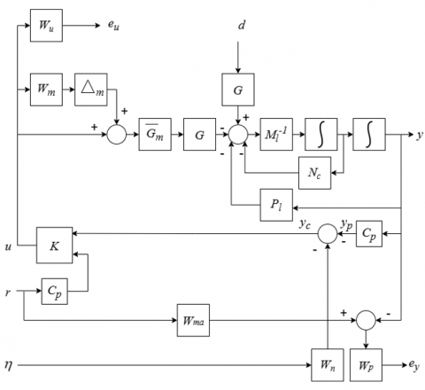
The suggested controller has two degrees of freedom as depicted in Figure 2 [25], where, r represents the reference input, K represents the controller, u represents the control action, d represents the disturbance, Gmodelrepresents the model, y represents the output, h represents the measurement noise, and yc represents the fed back measured output (affected by noise).
Figure 2. Two degrees of freedom control configuration
The controller K constitutes of two parts, K=[Kr Ky]T, where Kr is a prefilter and Ky is the feedback controller. It has six inputs (three reference signals and three measured angles) and two outputs (inputs to actuators).
3.1 Synthesizing the H-infinity controller
The two degrees of freedom control system in Figure 2 can be utilized to control the modeled triple inverted pendulum system as shown in Figure 3.
Figure 3. Triple inverted pendulum control system
The input voltage to the DC motors is obtained by:
$u(s)=K(s)\left[\begin{array}{c}y_c(s) \\ C_p r(s)\end{array}\right]$ (6)
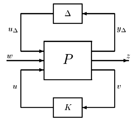
To design an H-infinity controller, the two degrees of freedom control configuration in Figure 3 has to be in the general robust control configuration of Figure 4 where $P$ represents the generalized plant model. $\Delta$ represents the normalized model uncertainty $\left(\|\Delta\|_{\infty}<1\right)$, $u$ represents the control signals, $w$ represents the weighted exogenous signals ($d, r$, and $\eta$) in Figure 3, $z$ represents the weighted error signals of interest ($e_u$ and $e_x$) in Figure 3.v represents the controller input ($y_s$ and $C_p r$). $u \Delta$ and $y_{\Delta}$ represent the perturbed input and output, respectively.
Figure 4. General control configuration
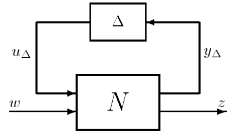
The stabilizing controller K in Figure 4 is to be synthesized for the generalized plant P to produce the control signals required for the actuators. During gamma-iteration, the minimal gamma is computed for which the condition:
$\min _K\|N\|_{\infty}<\gamma$ (7)
is satisfied, where $\gamma$ represents the H -infinity cost, and $N$ represents the lower linear fractional transformation of the closed-loop system defined by:
$N=F_l(P, K) \triangleq P_{11}+P_{12} K\left(I-P_{22} K\right)^{-1} P_{21}$ (8)
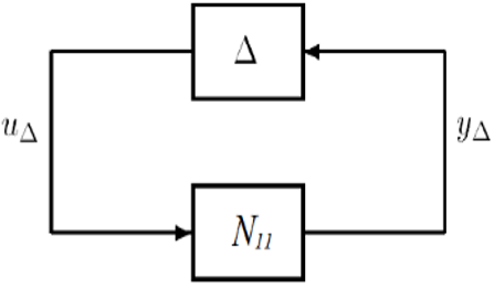
For robustness analysis of the designed control system, the structures in Figure 5 are used.
(a) N-D structure
(b) N11-D structure
Figure 5. Robustness analysis structures
Based on structured singular value (SSV) tool, the robust stability condition is given by Eq. (9) whereas the robust performance condition is given by Eq. (10) [25]:
$Robust \,Stability$ $\rightarrow \mu_{\Delta}\left(N_{11}\right)<1$ (9)
$Robust \,Performance$ $\rightarrow \mu_{\Delta}(N)<1$ (10)
for all frequencies, where, N11 is the transfer function from the output to the input of the perturbations.
3.2 Optimizing the performance weighting transfer matrix
In H-infinity controller design, PWTM plays a crucial role in determining the trade-off between various control objectives. It is used to find a controller that balances system performance with robustness to uncertainties. PSO offers an effective way to optimize this weighting matrix, and the cost function formulation directly guides this optimization process.
The coefficients of the PWTM are to be determined by PSO technique to achieve robust performance and stability. The transfer functions are to be of second order then the total parameters to be optimized for a diagonal performance weighting transfer matrix is 21 (3 transfer functions each has 3 numerator coefficients, 3 denominator coefficients, and a gain).
PSO is a simple and flexible swarm-intelligence-based algorithm that has been used in a wide variety of applications [27]. Since PSO is capable of searching for optimal solutions in complex, non-linear problems effectively, it is a good fit for application in control design. In controller development, PSO can be used to find the optimal parameters of specific design variables by spreading solutions randomly within the search space then directing them towards the solution that minimizes a predetermined cost function.
The PSO algorithm searches for the optimal solution to a cost function by adjusting the trajectories of individual particles. The cost function of the design problem is multi-objective. To meet the control goals of this paper, the cost function of the optimization problem has to include the Integral Time Absolute Error (ITAE) of the three links' angles and the structured singular values of the closed loop control systems in Figure 5. Using the Weighted-sum method, the cost function is suggested to be:
$\begin{aligned} & \text { Cost function }=0.25 \times[\text { ITAE1 }+ \text { ITAE2 }+ \text { ITAE3 }] \\ & +0.35 \times \max \left(\mu_{\Delta}\left(N_{11}\right)\right)+0.4 \times \max \left(\mu_{\Delta}(N)\right)\end{aligned}$ (11)
where,
$\operatorname{ITAE} 1=\int\left|e_1(t)\right| * t d t$ (12)
ITAE2 $=\int\left|e_2(t)\right| * t d t$ (13)
$\operatorname{ITAE} 3=\int\left|e_3(t)\right| * t d t$ (14)
where, e1, e2, and e3 represent the errors of links 1, 2, and 3, respectively.
Both the number of iterations and the swarm size are set to 20, cognitive coefficient (c1) and social coefficient (c2) to 2, minimum and maximum inertia weights (wmin and wmax) to 0.2 and 0.7, respectively, lower and upper bounds of the search space to 0.5 and 100, respectively, and number of variables to 21.
PSO algorithm starts by setting the initial particles' positions (Xi) randomly within the search space, the initial particles' velocities (Vi) to 0, where i indicates the iteration index. the particle's positions are then applied to the corresponding coefficients of the performance weighting transfer matrix. The H-infinity controller is then synthesized according to Eq. (7) and applied to the system to obtain output errors and the structured singular values. The cost function is computed as given in Eq. (11). The best personal solution of each particle (Pbest i) and the best global solution of all particles (Gbest) are then found according to the particles' score of the cost function. Next, the particles' velocities and positions are updated according to:
$\begin{gathered}V_i(t+1)=w \times V_i(t)+c_1 \times \operatorname{rand}_1 \times \\ \left(P_{\text {best } i}(t)-X_i(t)\right)+c_2 \times \operatorname{rand}_2 \times\left(G_{\text {best }}(t)-X_i(t)\right)\end{gathered}$ (15)
$X_i(t+1)=X_i(t)+V_i(t+1)$ (16)
where, w represents the inertia weight, rand1 and rand2 are two random numbers between 0 and 1.
The algorithm repeats itself till maximum number of iterations is reached. The final controller can then be applied to the original nonlinear system. The proposed merging of PSO with the H-infinity controller design is depicted in Figure 6.
Figure 6. The proposed controller design steps
Figure 7. Closed loop system's poles
The designed controller is of order 30 and achieves γ=0.6464. The poles of the closed loop system lie in the left half plane as shown in Figure 7 which indicates decaying exponential responses and hence, indicates system's stability.
The PWTM obtained by optimization is given by:
$W p(s)=\left[\begin{array}{ccc}0.5 \frac{0.5 s^2+43.194 s+100}{65.093 s^2+100 s+83.942} & 0 & 0 \\ 0 & 60.159 \frac{36.253 s^2+100 s+89.199}{54.033 s^2+53.279 s+0.5} & 0 \\ 0 & 0 & 0.5 \frac{43.644 s^2+19.887 s+65.851}{0.5 s^2+60.372 s+13.465}\end{array}\right]$
The developed control system with the optimized PWTM is to be tested in section 5. It is also to be compared to the control system with the unoptimized PWTM given by [1]:
$W p(s)=\left[\begin{array}{ccc}0.01 \frac{s^2+2 s+4}{s^2+1.5 s+0.1} & 0 & 0 \\ 0 & 0.02 \frac{s^2+2 s+4}{s^2+1.5 s+0.01} & 0 \\ 0 & 0 & 0.04 \frac{s^2+2 s+4}{s^2+1.5 s+0.01}\end{array}\right]$
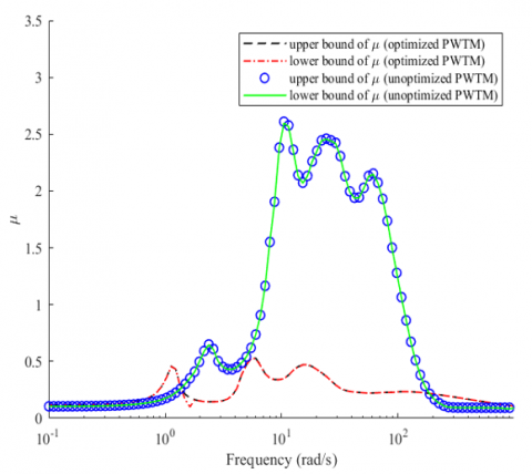
The structured singular values μ∆ (N11) of the developed closed loop control system with optimized and unoptimized PWTM are shown in Figure 8. The upper bound of μ of the developed closed loop control system with optimized PWTM satisfies condition (9) since the max (μ∆ (N11)) is 0.528. Hence, the uncertain closed loop system is robustly stable and can tolerate up to 188% of the modeled uncertainty.
Figure 8. Upper and lower bounds of μ∆ (N11)
Table 1. Stability robustness sensitivity
|
Parameter |
Sensitivity in Optimal PWTM |
Sensitivity in Non-Optimal PWTM |
|
first actuator uncertain dynamics |
51% |
54% |
|
second actuator uncertain dynamics |
30% |
21% |
|
first hinge's viscous friction coefficient |
1% |
0% |
|
second hinge's viscous friction coefficient |
0% |
0% |
|
third hinge's viscous friction coefficient |
1% |
0% |
|
first motor's viscous friction coefficient |
6% |
15% |
|
second motor's viscous friction coefficient |
1% |
0% |
|
first link's moment of inertia around the center of gravity |
19% |
23% |
|
second link's moment of inertia around the center of gravity |
1% |
8% |
|
third link's moment of inertia around the center of gravity |
62% |
31% |
Figure 9. Upper and lower bounds of μ∆ (N)
Table 2. Performance robustness sensitivity
|
Parameter |
Sensitivity in Optimal PWTM |
Sensitivity in Non-Optimal PWTM |
|
first actuator uncertain dynamics |
26% |
54% |
|
second actuator uncertain dynamics |
5% |
20% |
|
first hinge's viscous friction coefficient |
1% |
0% |
|
second hinge's viscous friction coefficient |
0% |
0% |
|
third hinge's viscous friction coefficient |
0% |
0% |
|
first motor's viscous friction coefficient |
3% |
15% |
|
second motor's viscous friction coefficient |
1% |
0% |
|
first link's moment of inertia around the center of gravity |
11% |
22% |
|
second link's moment of inertia around the center of gravity |
0% |
8% |
|
third link's moment of inertia around the center of gravity |
35% |
31% |
The upper bound of μ of the closed loop control system with unoptimized PWTM does not satisfy condition (9) since the max (μ∆ (N11)) is greater than 1, which means that the system is not stable for samples of the modeled perturbed set other than the nominal system (as will be shown in the next section).
The sensitivity of stability robustness to the uncertain parameters are given in Table 1. The robust stability is more dependent on uncertainties in moment of inertia of the third arm and the actuators uncertain dynamics. It is almost independent on uncertainties in viscous friction coefficients.
The robust stability margins of the optimal and non-optimal PWTM are 1.89 and 0.38, respectively. Which indicates greater tolerance for uncertainties in the optimized PWTM system before it becomes unstable. Hence, the optimal PWTM is more reliable than non-optimal PWTM in applications.
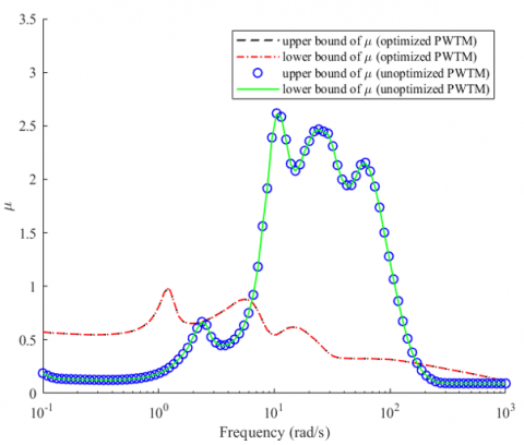
The structured singular values μ∆ (N) of the optimized and unoptimized PWTM closed loop control system are shown in Figure 9. Condition (10) is also satisfied in the optimized PWTM system since the max (μ∆ (N)) is 0.987. Hence, the uncertain closed loop system achieves performance robustness. A model uncertainty of 101% can lead to input/output gain of 0.986 at frequency 1.23 rad/sec. At any other frequency, the uncertain closed loop system has higher performance robustness.
The upper bound of μ of the closed loop control system with unoptimized PWTM does not satisfy condition (10) since the max (μ∆ (N11)) is greater than 1, which means that system uncertainty leads to degradation in performance.
Table 2 shows that the robust performance is moderately dependent on uncertainties in moment of inertia of the third link and the first actuator uncertain dynamics. It is almost independent on variations in viscous friction coefficients, moment of inertia of the second link and the second actuator uncertain dynamics. The robust performance margins of the optimal and non-optimal PWTM are 1.01 and 0.38, respectively. Which again indicates that the optimal PWTM can handle larger deviations from the nominal model while still achieving desired performance which is the essence of the controller development in this paper.
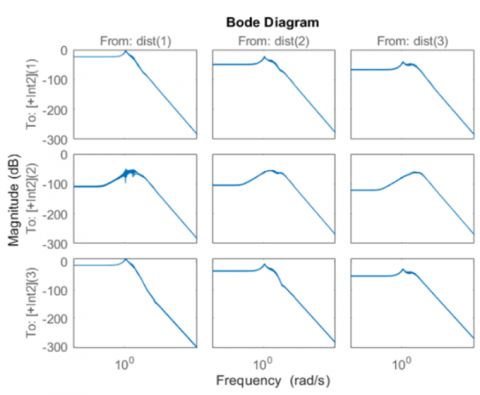
In order to investigate the system robustness against different scenarios of disturbances, the bode plots of the uncertain transfer functions from disturbance inputs to the three controlled angles are plotted in Figure 10. As can be seen, the maximum gain from any disturbance to any angle is below 0 dB, which means that over all the frequency range [10-5, 107 rad/sec], the disturbances are attenuated. Moreover, it can be seen that the disturbance attenuation level dramatically increases at high frequencies, which indicates that the control system can effectively filter out rapid fluctuations in the disturbance signal.
Figure 10. Disturbance frequency response
It can also be concluded from this plot that when a disturbance is applied at the first link, its effect on the first and third angles is the least attenuated (maximum gain is almost 0 dB at 1 rad/sec).
In this section, the stabilizing and tracking problems of the triple inverted pendulum system are investigated. Meanwhile, the robustness of the control system under uncertain parameters' variations, disturbance, and noise are analyzed. Also, the results of different cases are given. A comparison with the unoptimized PWTM control system is made throughout the cases. The results are simulated using MATLAB.
5.1 Case 1 (Stabilization)
To check the system's ability to robustly overcome the effect of parameters' variations, 30 samples of uncertain models (within the model uncertainty range) are tested. The stabilization of the system in the upright position requires all links to be aligned vertically (θ1d=θ2d=θ3d=0 deg) in the presence of external torque disturbance on the third link (d3=0.1 N.m) and measurement noise in all potentiometers (h1=h2=h3=±0.5 V). The closed-loop response of the system is shown in Figure 11.
The responses of 30 samples of the uncertain models in Figure 11(a) are almost identical (the discrepancies in all angles' due to parameters' variations are unrecognizable). It is noted that θ1 and θ2 responses are smoother than θ3 response. Yet, the wobbles of θ3 around the desired value are of very small amplitude (0.859 deg=0.015 rad). Figure 11(b) shows that the unoptimized PWTM system response cannot stay stable for all samples within the modeled perturbed set (the responses of θ2 and θ3 exhibits similar unstable behavior and their plots are not included to save space).
(a) Optimized PWTM
(b) First link angle (optimized and unoptimized PWTM)
Figure 11. Closed-loop response (case 1)
(a) Optimized PWTM
(b) First control signal (optimized and unoptimized PWTM)
Figure 12. Control action (case 1)
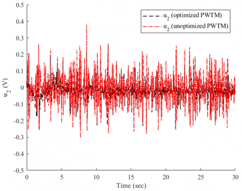
Figure 12(a) shows the control action produced by the developed controller. To keep the angles at their desired value, the controller signals fluctuate to compensate the effect of noise on potentiometers' readings. In the same time, they tend to reject disturbance and attain the desired response in spite of variations in uncertain parameters in the model and actuators. The control action u2 plays major role in achieving this goal.
Figure 12(b) shows that the unoptimized PWTM is practically inefficient compared to the optimized PWTM system.
5.2 Case 2 (Stabilization)
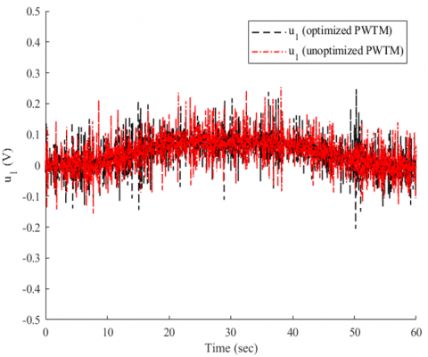
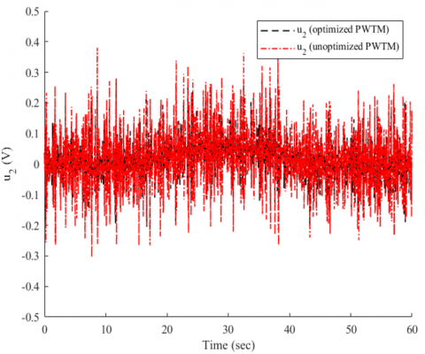
To test the robustness of the original nominal nonlinear system, consider applying disturbance and measurement noise to every link of the nonlinear system. The disturbances are applied asynchronously to all the three links (d1 at t=0 sec, d2 at t=5 sec, and d3 at t=10 sec). The nonlinear system responds as shown in Figure 13.
In the optimized PWTM system, the angle of the first link θ1 oscillates before settling with steady state error=0.401 deg (0.007 rad). While θ2 follows the desired value without overshooting. θ3 in Figure 13(c) overshoots to 5.446 deg (0.095 rad) at t=1.809 sec then settles with steady state error=1.261 deg (0.022 rad).
The angles of all links are almost unaffected by the applied measurement noise in the system with optimized PWTM, while the effect of noise is not well compensated in the system with unoptimized PWTM. The control signals of case 2 are shown in Figure 14. u2 of optimized PWTM could compensate the effect of disturbance and noise with less effort than in unoptimized PWTM system.
(a) First link angle (optimized and unoptimized PWTM)
(b) Second link angle (optimized and unoptimized PWTM)
(c) Third link angle (optimized and unoptimized PWTM)
Figure 13. Closed-loop response (case 2)
(a) First control signal
(b) Second control signal
Figure 14. Control action (case 2)
5.3 Case 3 (Tracking)
To investigate the ability of tracking different references for each link, the following reference signals are applied: θ1d=5 deg for the time interval [5, 35) sec and θ1d= 0 deg in other time intervals, θ2d=-10 deg for the time interval [5, 40) sec and θ2d=0 deg in other time intervals, θ3d=-5 deg for the time interval [15, 35) sec and θ3d=0 deg in other time intervals.
(a) First link angle (optimized and unoptimized PWTM)
(b) Second link angle (optimized and unoptimized PWTM)
(c) Third link angle (optimized and unoptimized PWTM)
Figure 15. Closed-loop response (case 3)
Also, an 0.1 N.m external disturbance is applied to the second link at t=25 sec. In addition, noise is applied in all measurements readings. The nonlinear system responds as shown in Figure 15. The three angles θ1, θ2, and θ3 needs 20, 15, 10 seconds, respectively to follow the given references by the aid of the control signal shown in Figure 16. Unlike the unoptimized PWTM system response, the optimized system response is unaffected by noise. On the other hand, the effect of the applied disturbance at t=25 sec is manifested in the optimized PWTM system response of the third link yet, immediately rejected.
(a) First control signal
(b) Second control signal
Figure 16. Control action (case 3)
The rise and settling time (in seconds), maximum overshoot and steady-state error (in degrees) characteristics of all above cases are listed in Table 3. The results of simulating different cases of regulating and tracking of the control system under different conditions validate the effectiveness and robustness of the developed controller.
Table 3. Control system response specifications
|
Parameter |
Case 1 |
Case 2 |
Case 3 |
|
Rise time (first link) optimized PWTM |
0 |
0 |
15 |
|
Rise time (first link) unoptimized PWTM |
unstable |
1.67 |
15 |
|
Settling time (first link) optimized PWTM |
0 |
13.296 |
20 |
|
Settling time (first link) unoptimized PWTM |
unstable |
4 |
20 |
|
Maximum overshoot (first link) optimized PWTM |
0 |
0.046 |
0 |
|
Maximum overshoot (first link) unoptimized PWTM |
unstable |
0.288 |
0.225 |
|
Steady-state error (first link) optimized PWTM |
0 |
0.401 |
0.257 |
|
Steady-state error (first link) unoptimized PWTM |
unstable |
0.183 |
0.219 |
|
Rise time (second link) optimized PWTM |
0 |
0 |
11 |
|
Rise time (second link) unoptimized PWTM |
unstable |
0 |
11 |
|
Settling time (second link) optimized PWTM |
0 |
0 |
15 |
|
Settling time (second link) unoptimized PWTM |
unstable |
3.5 |
15 |
|
Maximum overshoot (second link) optimized PWTM |
0.197 |
0 |
0 |
|
Maximum overshoot (second link) unoptimized PWTM |
unstable |
1.906 |
0.555 |
|
Steady-state error (second link) optimized PWTM |
0 |
0.005 |
0 |
|
Steady-state error (second link) unoptimized PWTM |
unstable |
0.04 |
0.214 |
|
Rise time (third link) optimized PWTM |
0 |
0 |
7 |
|
Rise time (third link) unoptimized PWTM |
unstable |
0 |
7 |
|
Settling time (third link) optimized PWTM |
0 |
15 |
10 |
|
Settling time (third link) unoptimized PWTM |
unstable |
3 |
10 |
|
Maximum overshoot (third link) optimized PWTM |
0.678 |
5.446 |
0.348 |
|
Maximum overshoot (third link) unoptimized PWTM |
unstable |
1.528 |
0.495 |
|
Steady-state error (third link) optimized PWTM |
0.228 |
1.261 |
0.071 |
|
Steady-state error (third link) optimized PWTM |
unstable |
0.017 |
0.077 |
The developed controller has attained the robust stability and performance for the triple inverted pendulum system by optimizing the PWTM coefficients using PSO method. The key point was to include the structured singular values (that are required to be less than one in robustness conditions) with the tracking error in the cost function with suitable weights for each term. Considering the possible sources of uncertainty in the model, different cases of regulating and tracking were simulated. The results show that the controlled system is capable of handling all applied perturbation even when applied simultaneously. The most important achievement in this paper lies in the compromise between time response characteristics and robustness without exhibiting unnecessary conservativeness. It would be challenging to model a wider range of uncertainty and examine the robustness attaining ability of the proposed for higher uncertainty. In future, other robust control methods like Mu-synthesis can be also optimized in a suitable way to achieve further enhancements on robustness and performance. It is also recommended to implement the proposed control strategy on a system with multiple interconnected triple inverted pendulums in which maintaining stability becomes a bigger challenge.
|
C1 |
viscous friction coefficient of the first hinge, N. m. s |
|
C2 |
viscous friction coefficient of the second hinge, N. m. s |
|
C3 |
viscous friction coefficient of the third hinge, N. m. s |
|
Cm1 |
viscous friction coefficient of the first motor, N. m. s |
|
Cm2 |
viscous friction coefficient of the second motor, N. m. s |
|
$C_{p_1^{\prime}}$ |
viscous friction coefficient of the belt–pulley system of the first hinge, N. m. s |
|
$C_{p_2^{\prime}}$ |
viscous friction coefficient of the belt–pulley system of the second hinge, N. m. s |
|
h1 |
the distance from the bottom to the center of gravity of the first arm, m |
|
h2 |
the distance from the bottom to the center of gravity of the second arm, m |
|
h3 |
the distance from the bottom to the center of gravity of the third arm, m |
|
I1 |
moment of inertia of the first arm around the center of gravity, kg. m2 |
|
I2 |
moment of inertia of the second arm around the center of gravity, kg. m2 |
|
I3 |
moment of inertia of the third arm around the center of gravity, kg. m2 |
|
Im1 |
moment of inertia of the first motor, kg. m2 |
|
Im2 |
moment of inertia of the second motor, kg. m2 |
|
$I_{p_1^{\prime}}$ |
moment of inertia of the belt–pulley system of the first hinge, kg. m2 |
|
$I_{p_2^{\prime}}$ |
moment of inertia of the belt–pulley system of the second hinge, kg. m2 |
|
K1 |
dimensionless ratio of teeth of belt–pulley system of the first hinge |
|
K2 |
dimensionless ratio of teeth of belt–pulley system of the second, hinge |
|
l1 |
length of the first arm, m |
|
l2 |
length of the second arm, m |
|
m1 |
mass of the first arm, kg |
|
m2 |
mass of the second arm, kg |
|
m3 |
mass of the third arm, kg |
|
α1 |
gain of the first potentiometer, V. rad-1 |
|
α2 |
gain of the second potentiometer, V. rad-1 |
|
α3 |
gain of the third potentiometer, V. rad-1 |
[1] Gu, D., Petkov, P.H., Konstantinov, M.M. (2013). Robust Control Design with MATLAB. United Kingdom: Springer London.
[2] Fajar, M. (2014). Control of the two DoF inverted pendulum. Dinamika Teknik Mesin, 4(2): 71-77. http://doi.org/10.29303/d.v4i2.54
[3] Varghese, E., Vincent, A., Bagyaveereswaran, V. (2017). Optimal control of inverted pendulum system using PID controller, LQR and MPC. IOP Conference Series: Materials Science and Engineering, 263: 052007-052022. http://doi.org/10.1088/1757-899X/263/5/052007
[4] Ali, H., Kadhim, M. (2018). H2 sliding mode controller design for mobile inverted pendulum system. Iraqi Journal of Computers, Communications, Control and Systems Engineering, 18(2): 17-29. https://doi.org/10.33103/uot.ijccce.18.2.2
[5] Abut, T. (2023). Optimal LQR controller methods for double inverted pendulum system on a cart. DÜMF Mühendislik Dergisi, 14(2): 247-255. http://doi.org/10.24012/dumf.1253331
[6] Tran, V.D., Ho, T.N., Nguyen, M.T., Nguyen, V.D.H. (2017). Balancing control for double-linked inverted pendulum on cart: Simulation and experiment. Journal of Technical Education Science, 12(2): 68-75. https://jte.edu.vn/index.php/jte/article/view/382.
[7] Krishna, B., Chandran, D., George, V., Thirunavukkarasu, I. (2015). Modeling and performance comparison of triple PID and LQR controllers for parallel rotary double inverted pendulum. International Journal of Emerging Trends in Electrical and Electronics, 11(2): 145-150.
[8] Phan, M.S., Do, T.C., Truong, V.Q., Nguyen, T.V.A. (2023). Comparative analysis of SMC-LMI and LQR controllers for double inverted pendulum. Journal of Measurement, Control, and Automation, 4(3): 1-7.
[9] Yi, Z., Peisi Z., Chao. Y.Q. (2016). Double inverted pendulum based on LQG optimal control. In Proceedings of the 2016 International Conference on Automatic Control and Information Engineering, pp. 83-87. http://doi.org/10.2991/icacie-16.2016.20
[10] Elkinany, B., Alfidi, M., Chaibi, R., Chalh, Z. (2020). T-S fuzzy system controller for stabilizing the double inverted pendulum. Advances in Fuzzy Systems, 2020(1). http://doi.org/10.1155/2020/8835511
[11] Moysis, L. (2016). Balancing a double inverted pendulum using optimal control and Laguerre functions. Technical Report. Aristotle University of Thessaloniki, Greece. http://doi.org/10.13140/RG.2.1.2948.6486
[12] Tijani, T., Jimoh, I. (2021). Optimal control of the double inverted pendulum on a cart: A comparative study of explicit MPC and LQR. Applications of Modelling and Simulation, 5: 74-87.
[13] Gustafsson, F.K. (2016). Control of inverted double pendulum using reinforcement learning. Stanford CS229 - Machine Learning. https://cs229.stanford.edu/proj2016/report/Gustafsson-ControlOfInvertedDoublePendulumUsingReinforcementLearning-report.pdf.
[14] Maraslidis, G.S., Kottas, T.L., Tsipouras, M.G., Fragulis, G.F. (2022). Design of a fuzzy logic controller for the double pendulum inverted on a cart. Information, 13(8): 379. http://doi.org/10.3390/info13080379
[15] Idrees, M., Ullah, Z., Younis, J., Ahmad, S., Ahmad, H. (2023). Stabilization of double inverted pendulum systems based on hierarchical sliding mode control techniques. Mathematical Problems in Engineering, 2023(1). http://doi.org/10.1155/2023/3916279
[16] Glück, T., Eder, A., Kugi, A. (2013). Swing-up control of a triple pendulum on a cart with experimental validation. Automatica. 49(3): 801-808. http://doi.org/10.1016/j.automatica.2012.12.006
[17] Sharma, K., Sahu V. (2016) Modeling and stabilization of cart triple link inverted pendulum using LQR controller incorporating degree of stability. International Research Journal of Advanced Engineering and Science. 1(4): 148-152.
[18] Setka, V., Cecil, R., Schlegel, M. (2017). Triple inverted pendulum system implementation using a new ARM/FPGA control platform. In 2017 18th International Carpathian Control Conference (ICCC), Sinaia, Romania, pp. 321-326, http://doi.org/10.1109/CarpathianCC.2017.7970419
[19] Ali, H.I. (2018). H-infinity model reference controller design for magnetic levitation system. Engineering and Technology Journal, 36(1): 17-26. http://doi.org/10.30684/etj.2018.136750
[20] Ali, H., Samir, K. (2014). H-infinity based active queue management design for congestion control in computer networks. In the Second Engineering Conference on Control, Computers and Mechatronics Engineering (ECCCM2, 2014), pp. 1-9.
[21] Singh, N., Bhangal, K. (2017). Robust control of double inverted pendulum system. Journal of Automation and Control Engineering, 5(1): 14-20. http://doi.org/10.18178/joace.5.1.14-20
[22] Sanjeewa, S.D., Parnichkun, M. (2019). Control of rotary double inverted pendulum system using mixed sensitivity H∞ controller. International Journal of Advanced Robotic Systems, 16(2). http://doi.org/10.1177/1729881419833273
[23] Ali, H.I., Hasan, A.F., Jassim. H.M. (2020). Optimal H2PID controller design for human swing leg system using cultural algorithm. Journal of Engineering Science and Technology, 15(4): 2270-2288.
[24] Tayyeh, I.F., Ali, H.I. (2022). Full state feedback H-infinity controller design for nonlinear systems. Journal Européen des Systèmes Automatisés, 55(4): 503-509. http://doi.org/10.18280/jesa.550409
[25] Skogestad, S., Postlethwaite, I. (2005). Multivariable Feedback Control: Analysis and Design. John Wiley & Sons.
[26] Shafeek, Y.A., Ali, H.I. (2024). Balancing of robustness and performance for triple inverted pendulum using μ-synthesis and gazelle optimization. Journal Européen des Systèmes Automatisés, 57(2): 443-452. http://doi.org/10.18280/jesa.570214
[27] Yang, X. (2014). Nature-Inspired Optimization Algorithms. London, Elsevier.