Amir Abdul Majid![]()
© 2025 The author. This article is published by IIETA and is licensed under the CC BY 4.0 license (http://creativecommons.org/licenses/by/4.0/).
OPEN ACCESS
This study aims to evaluate the sensitivity of photovoltaic (PV) solar cell parameters, using adjoint network analysis based on Tellegin’s theorem, to provide critical insights into the factors that influence the performance of solar cells. Key parameters such as irradiance, material properties, series and shunt resistance, load resistance matching, and voltage-current characteristics determine the efficiency and power output of PV cells. By optimizing these sensitive parameters, manufacturers can improve PV cell performance, reduce energy losses, and increase the overall efficiency of solar panels. A mathematical formulation based on Tellegen’s theorem is adopted to evaluate the sensitivity of parameters used in PV cell manufacturing. The implemented sensitivity method is accurate up to 1% compared with the Central Finite Difference (CFD) method. The simulation of the PV cell and its adjoint circuit have been evaluated for currents and voltages to be used in the derived sensitivity formulation. The range of sensitivities of the output voltage has been evaluated and found largely constant with variations of the PV cell parameters around their nominal values estimated at the optimal output power V-I characteristic point.
adjoint circuits, optimization, PV parameters, sensitivity, Tellegen’s theorem
1.1 Background
Photovoltaic (PV) cells are the building blocks of solar panels, which convert sunlight directly into electricity through the photovoltaic effect. As the demand for clean, renewable energy grows, understanding and optimizing the performance of PV solar cells becomes increasingly important. A sensitivity study of PV solar cell parameters helps in identifying how changes in these parameters affect the efficiency, power output, and reliability of solar cells. This essay will explore key parameters that influence the performance of PV cells, such as irradiance, temperature, material properties, and internal resistances, and analyze their sensitivity to changes.
A PV solar cell consists of semiconductor materials, typically silicon, that absorb photons from sunlight. When these photons strike the cell, they excite electrons, which create a flow of electric current. The PV solar cell's performance depends on various parameters, including external factors like temperature and sunlight intensity and internal characteristics such as material properties and resistances. In practical applications, solar panels consist of many PV cells connected in series or parallel configurations to achieve the desired power output. The efficiency of a PV system depends on how well each individual cell performs, which makes a detailed sensitivity study essential to optimize overall energy yield. Several parameters determine the efficiency and output of PV cells, and each is sensitive to variations in conditions and design choices. These include:
Shunt resistance (Rsh), on the other hand, represents leakage pathways within the cell, where current bypasses the load and circulates within the cell itself. Low shunt resistance reduces the cell's ability to maintain voltage, especially under low-light conditions, leading to power losses. Ideally, shunt resistance should be as high as possible to minimize these losses. Both series and shunt resistances are key parameters in determining the fill factor of the PV cell, which is a measure of how closely the cell's power output matches its theoretical maximum.
We shall concentrate in this study on PV cell circuits and external properties, namely sensitivity to series and parallel resistances, as well as diode effect resistance and load resistance. Other effect sensitivities exist as well such as sensitivity to material properties and temperature, in which the former is related to the doping concentration of the semiconductor material, and the latter can have a significant impact on PV cell efficiency, primarily affecting the open-circuit voltage (Voc). As temperature increases, the energy required for electrons to cross the bandgap decreases, leading to a reduction in Voc. In contrast, the short-circuit current (Isc) increases slightly with temperature because more thermal energy is available to excite electrons. However, the overall effect of increased temperature is a reduction in efficiency, as the decrease in Voc outweighs the small gain in Isc.
1.2 Literature survey
The several parameters of PV solar cell such as irradiation, series and shunt resistances, I-V characteristic, and load resistance, all constitute major effects on sensitivity [1], optimization [2], and reliability [3]. An early work on network sensitivity using a generalized adjoint concept [3] was attempted in 1969, and later this concept was adopted for time domain TLM application [4]. A feasible sensitivity technique for EM design optimization [5] is applied for electrical engineering topics. Similarly, a time-domain adjoint variable method for materials with dispersive parameters is presented [6]. The work conducted by Georgieva et al. [7] was to investigate feasible adjoint sensitivity technique for EM design optimization.
Since the aim is to study the sensitivity of PV solar cell parameters, the work [8] has been checked for the sensitivity analysis of photovoltaic cells under different conditions. A further attempt is presented to study PV cell parameter extraction using variable reduction and improved shark optimization technique [9]. Similar work is attempted to design an optimal model parameters estimation of solar and fuel cells using an estimation algorithm [10]. A random forest model for global sensitivity analysis [11] is presented for general applications. Antoniadis et al. [12] analyzed the global sensitivity of PV cell parameters based on credibility variances. A sensitivity and reliability model for a PV system connected to a grid [13], and the published work for a detailed sensitivity solution of PV solar cell [14] are found to be useful to our work. Other literature work was found advantageous, namely the work of Praene et al. [15] to optimize a solar absorption cooling system and the novel procedures for identifying single-diode models of PV cells [16]. The work of Shaik et al. [17] is an experimental review to investigate the effect of various parameters on the performance of solar PV power plant: a review and experimental, while Mesbahi et al. [18] are using a new sensitivity approach to photovoltaic parameters extraction based on the total least squares method. Another sensitivity approach using photovoltaic parameters extraction which based on the total least squares method was analyzed by Chowdhury et al. [19]. The effect of PV sensitivity analysis to environmental factors was studied by Ziar and Karegar [20]. The work of Verma et al. [21] is a special sensitivity analysis of solar PV system for different PV array configurations.
1.3 Motivation
To predict the sensitivity of PV cells with respect of different parameters, related or independent, which makes the calculation lengthy and time-consuming. Instead, we try to use theoretical theorems and mathematical manipulation to evaluate the overall sensitivity efficiently. The advantage of adjoint sensitivity analysis is using only one extra circuit simulation of the adjoint circuit to evaluate the sensitivities of the desired objective function with respect to all desired circuit parameters regardless of their number. To validate the accuracy of the method used, the Central Finite Difference (CFD) method is to be implanted. The adjoint network analysis method can detect the sensitivity of the output voltage to any parameter variable only once without the need to run the analysis several times for different perturbations, as used in the CFD method. This process will help PV cell manufacturers to select optimized values of series, shunt, diode resistance as well as load resistance operating at maximum output power of the Voltage-current characteristics.
1.4 Contribution
The influence of several dominant parameters on the output voltage and consequently power and efficiency, is studied by using the sensitivity analysis method based on adjoint network theory. These parameters are equivalent series resistance, and equivalent parallel resistance, as well as irradiation intensity, photovoltaic cell surface temperature, temperature coefficient [9, 13]. The analysis must be repeated for each parameter and for each parameter perturbation value, which consumes time and resources. The systematic solution method [14] is to obtain the five-parameter model in case of only a few data (Voc, Isc, Vmp, and Imp) available from the manufacturers. In this work, the sensitivities of parameters are graphically analyzed on condition that as few simplifications as possible are made, which involves solving the nonlinear equation system through iterative computations, which cannot ensure accurate results. Another approach [16] proposes a novel fitting procedure that identifies both single-diode model parameters and PV module temperature and irradiance utilizing an iterative. The procedure enables degradation and aging analyses using only the internal electrical current-voltage curve measurements of the inverter. This approach is especially suitable for detecting aging, and confirming the functionality of the procedure for condition monitoring. Our work is based on adjoint sensitivity which ensures accurate results for any number of parameters and for any perturbations. This can for example, performed with one MATLAB simulation instead of multiple simulation runs.
A mathematical formulation based on Tellegen’s theorem is adopted to evaluate the sensitivity for parameters used in PV cell manufacturing. The method is accurate up to 1% compared with the Central Finite Difference method (CFD). The simulation of PV cell and its adjoint circuit have been evaluated for currents and voltages to be used in the derived sensitivity formulation. Variations of series and shunt resistances as well as the PV cell dark diode resistance and load conditions, are to be tested for the evaluated sensitivity verification. This method can be extended to other sensitivity applications such as wind turbine and other renewable energy systems.
Tellegen’s theorem states that the conservation of instantaneous power of any network made up of parallel and series branches, applies to two different circuits that have the same topologies. The electric circuit is a network of branches of electrical elements, which is used here. It is needed to find the equivalent circuit of any device or equipment in order to use this concept by finding an adjoint circuit to the original one having same structure of circuit branches. The sensitivity of the PV cell equivalent circuit due to variations in the circuit elements can be analyzed using the adjoint network method based on Tellegen’s theorem in which the branch voltages and currents vary with the circuit elements such as resistors, capacitors, and inductors. It is assumed to estimate the sensitivities of the current drawn from a voltage source or voltage across a current source, with respect to all desired parameters. According to the conservation of power of any electric circuit:
$v^T i=v_1 i_1+v_2 i_2+\cdots+v_N i_N=0$ (1)
where, ij and vj are the current and voltage of the jth branch, and N is the number of branches. If Ĩ and Ṽ are vectors of currents and voltages of another circuit, i.e., an adjoint circuit, with the same topology at a certain frequency, then:
$\tilde{\mathrm{I}}^{\mathrm{T}} \tilde{\mathrm{V}}=0$ and $\tilde{\mathrm{V}}^T \tilde{\mathrm{I}}=0$ (2)
Combining Eq. (2) leads to:
$\tilde{\mathrm{I}}^T \tilde{\mathrm{V}}-\tilde{\mathrm{V}}^T \tilde{\mathrm{I}}=0$ (3)
Eq. (3) can be written for each branch as:
$\sum_{k=1}^N V_k \tilde{\mathrm{I}}_k-\sum_{k=1}^N {I}_k \tilde{\mathrm{V}}_k=0$ (4)
We shall generalize Eq. (4) for all current and voltage sources and branch elements, as:
$\begin{gathered}\sum_{v-{ sources }}\left(V_k \tilde{\mathrm{I}}_k-I_k \tilde{V}_k\right)+\sum_{i- { sources }}\left(V_k \tilde{\mathrm{I}}_k-I_k \tilde{V}_k\right) \sum_{{elements }}\left(V_k \tilde{\mathrm{I}}_k-I_k \tilde{V}_k\right)=0\end{gathered}$ (5)
When one element in the original circuit varies, the currents drawn from voltage sources will change and similarly for the voltages across current sources, yet the currents from current sources or the voltages across voltage sources don’t change because they are independent sources. Hence Eq. (5) can be written as:
$\begin{gathered}\sum_{v- { sources }}\left(V_k \tilde{\mathrm{I}}_k-\left(I_k+\Delta I_k\right) \tilde{\mathrm{V}}_k\right)+ \sum_{i- { sources }}^i\left(\left(V_k+\Delta V_k\right) \tilde{\mathrm{I}}_k-I_k \tilde{\mathrm{~V}}_k\right)+ \sum_{ {elements }}\left(\left(V_k+\Delta V_k \tilde{\mathrm{I}}_k-\left(I_k+\Delta I_k\right) \tilde{\mathrm{V}}_k\right)=0\right.\end{gathered}$ (6)
Subtracting Eq. (5) from (6), leads:
$\begin{aligned} & -\sum_{v- { sources }}\left(\Delta I_k \tilde{V}_k\right)+\sum_{i-{ sources }}\left(\Delta V_k \tilde{\mathrm{I}}_k\right) \quad+\sum_{ {elements }}\left(\Delta V_k \tilde{\mathrm{I}}_k-\Delta I_k \tilde{\mathrm{~V}}_k\right)=0\end{aligned}$ (7)
Rearranging and dividing both sides of Eq. (7) by $\Delta x_i$ which is any perturbation in the circuit elements, and limiting $\Delta x_i$ to small value, leads to:
$\begin{gathered}\sum_{v- { sources }}\left(\frac{\partial I_k}{\partial x_i} \tilde{V}_k\right)-\sum_{i-{ sources }}\left(\frac{\partial V_k}{\partial x_i} \tilde{\mathrm{I}}_k\right) =\sum_{ {elements }}\left(\frac{\partial V_k}{\partial x_i} \tilde{\mathrm{I}}_k-\frac{\partial I_k}{\partial x_i} \tilde{V}_k\right)\end{gathered}$ (8)
An adjoint circuit can be constructed so that only one derivative exists on the left-hand side of the above equation is excited. We shall also impose special conditions on the adjoint circuit to remove the right-hand side of the equation since they are unknown.
In electric circuits, the relationships between voltages and currents are linear, and hence the general formulation of voltages and currents can be written as follows:
$\left[\begin{array}{c}I_a \\ V_b\end{array}\right]=\left[\begin{array}{cc}\boldsymbol{Y} & \boldsymbol{A} \\ \boldsymbol{M} & \boldsymbol{Z}\end{array}\right]\left[\begin{array}{l}V_a \\ I_b\end{array}\right]$ (9)
where, $V_a$, $V_b$, $I_a$ and $I_b$ are the subsets of voltages and currents of branches of any hybrid circuit. Differentiating Eq. (9) with respect to the $x_i$, leads:
$\left[\begin{array}{l}\frac{\partial I_a}{\partial x_i} \\ \frac{\partial V_b}{\partial x_i}\end{array}\right]=\left[\begin{array}{ll}\boldsymbol{Y} & \boldsymbol{A} \\ \boldsymbol{M} & \boldsymbol{Z}\end{array}\right]\left[\begin{array}{l}\frac{\partial V_a}{\partial x_i} \\ \frac{\partial I_b}{\partial x_i}\end{array}\right]+\left[\begin{array}{ll}\frac{\partial \boldsymbol{Y}}{\partial x_i} & \frac{\partial \boldsymbol{A}}{\partial x_i} \\ \frac{\partial \boldsymbol{M}}{\partial x_i} & \frac{\partial \boldsymbol{Z}}{\partial x_i}\end{array}\right]\left[\begin{array}{c}V_a \\ I_b\end{array}\right]$ (10)
Before substituting Eq. (10) into (8), we rearrange (8) to be:
$\begin{aligned} & \sum_{v- { sources }}\left(\frac{\partial I_k}{\partial x_i} \tilde{\mathrm{~V}}_k\right)-\sum_{i-{ sources }}\left(\frac{\partial V_k}{\partial x_i} \tilde{\mathrm{I}}_k\right)=\left[\begin{array}{c}\frac{\partial I_a}{\partial x_i} \\ \frac{\partial V_b}{\partial x_i}\end{array}\right]\left[\begin{array}{c}-\tilde{\mathrm{V}}_a \\ \tilde{\mathrm{I}}_b\end{array}\right]+\left[\begin{array}{c}\frac{\partial V_a}{\partial x_i} \\ \frac{\partial I_b}{\partial x_i}\end{array}\right]\left[\begin{array}{c}\tilde{\mathrm{I}}_a \\ -\tilde{\mathrm{V}}_b\end{array}\right]\end{aligned}$ (11)
Now substituting Eq. (10) into Eq. (11) and rearranging:
$\begin{aligned} & \sum_{v- { sources }}\left(\frac{\partial I_k}{\partial x_i} \tilde{\mathrm{V}}_k\right)-\sum_{i- { sources }}\left(\frac{\partial V_k}{\partial x_i} \tilde{\mathrm{I}}_k\right) = {\left[\begin{array}{l}\frac{\partial V_a}{\partial x_i} \\ \frac{\partial I_b}{\partial x_i}\end{array}\right]^T[\boldsymbol{F}]+\left[\begin{array}{l}V_a \\ I_b\end{array}\right]^T\left[\begin{array}{cc}\frac{\partial \boldsymbol{Y}^T}{\partial x_i} & \frac{\partial \boldsymbol{M}^T}{\partial x_i} \\ \frac{\boldsymbol{\partial} \boldsymbol{A}^T}{\partial x_i} & \frac{\partial \boldsymbol{Z}^T}{\partial x_i}\end{array}\right]\left[\begin{array}{c}-\tilde{\mathrm{V}}_a \\ \tilde{\mathrm{I}}_b\end{array}\right] }\end{aligned}$ (12)
where, F is:
$\boldsymbol{F}=\left[\begin{array}{ll}\boldsymbol{Y}^{\boldsymbol{T}} & \boldsymbol{M}^{\boldsymbol{T}} \\ \boldsymbol{A}^{\boldsymbol{T}} & \boldsymbol{Z}^{\boldsymbol{T}}\end{array}\right]\left[\begin{array}{c}-\tilde{\mathrm{V}}_a \\ \tilde{\mathrm{I}}_b\end{array}\right]+\left[\begin{array}{c}\tilde{\mathrm{I}}_a \\ -\tilde{\mathrm{V}}_b\end{array}\right]$ (13)
We shall make F=0 in order to get the unknown branch voltage and current equations without their derivatives. This will enforce the following condition on the adjoint circuit:
$\left[\begin{array}{cc}\boldsymbol{Y}^{\boldsymbol{T}} & -\boldsymbol{M}^{\boldsymbol{T}} \\ -\boldsymbol{A}^{\boldsymbol{T}} & \boldsymbol{Z}^{\boldsymbol{T}}\end{array}\right]\left[\begin{array}{l}\tilde{\mathrm{V}}_a \\ \tilde{\mathrm{I}}_b\end{array}\right]=-\left[\begin{array}{c}\tilde{\mathrm{I}}_a \\ \tilde{\mathrm{~V}}_b\end{array}\right]$ (14)
which simplifies the adjoint network relationship between the branch voltages and currents. Hence Eq. (12) can be simplified to be an efficient sensitivity relationship as:
$\begin{gathered}\sum_{v {-sources }}\left(\frac{\partial I_k}{\partial x_i} \tilde{\mathrm{V}}_k\right)-\sum_{i-{ sources }}\left(\frac{\partial V_k}{\partial x_i} \tilde{\mathrm{I}}_k\right) =\left[\begin{array}{l}V_a \\ I_b\end{array}\right]^T\left[\begin{array}{rr}-\frac{\boldsymbol{\partial} \boldsymbol{Y}^{\boldsymbol{T}}}{\partial x_i} & \frac{\boldsymbol{\partial} \boldsymbol{M}^{\boldsymbol{T}}}{\partial x_i} \\ -\frac{\boldsymbol{\partial \boldsymbol { A } ^ { \boldsymbol { T } }}}{\partial x_i} & \frac{\boldsymbol{\partial \boldsymbol { Z } ^ { T }}}{\partial x_i}\end{array}\right]\left[\begin{array}{c}\tilde{\mathrm{V}}_a \\ \tilde{\mathrm{I}}_b\end{array}\right]\end{gathered}$ (15)
It can be deduced from Eq. (13) that all sensitivities with respect to all circuit parameters can be evaluated regardless of the number of the n parameters, using both one adjoint simulation to find $\left[\begin{array}{ll}\tilde{\mathrm{V}}_a \tilde{\mathrm{I}}_b\end{array}\right]^T$ and one original simulation of the circuit $\left[V_a I_b\right]^T$. The derivatives of the metrices Y, M, A, and Z are analyzed according to the circuit topology. We can select the sensitivity of either the voltage across a current source or current drawn from a voltage source. This can be done by properly selecting the corresponding excitation in the adjoint network.
With this sensitivity study, the performance of PV can be improved by enhancing the manufacturing processes used for them. It can be seen from the equivalent circuit of a PV cell, that different ranges of circuit component values can exist due to their variations and hence, it is needed to select values that make the sensitivity of the output voltage to these parameters’ variations minimum.
To evaluate the sensitivity of the current drawn from the $j$ th voltage source, i.e., $\partial I_j / \partial x_i$, we set the related voltage excitation in the adjoint network $\tilde{V}_j=1.0 \mathrm{~V}$ with disabling al other adjoint sources, which means that all branche corresponding to voltage sources in the original circuit are shorted to ground in the adjoint network. Similarly, open al branches which corresponds to current sources in the origina circuit. It follows that the desired objective function determines the excitation of the adjoint circuit. On the othe hand, to get the sensitivity of the voltage across the $j$ th current source $\partial V_j / \partial x_i$, we set the corresponding excitation in the adjoint problem $\tilde{I}_j=1.0 \mathrm{~A}$ and all adjoint sources are set to zero To apply the above theory on PV cell sensitivity, the equivalent circuit of PV cell is shown in Figure 1.
(a)
(b)
(c)
Figure 1. (a) Equivalent circuit of a PV solar cell with adjoint circuit, (b) Thevenin’s equivalent, (c) Adjoint circuit
Figure 1(a) shows simulation of a PV cell with the dark diode represented by a 0.7 V battery in series with resistance Rd of typical value of 10-1000 Ω. Both Rs and Rshcan be approximately estimated from the current-voltage characteristic of the PV cell as:
$R_s \leq \frac{0.1 V_{o c}}{I_{s c}}, R s h \geq \frac{10 V_{o c}}{I_{s c}}$
where, $V_{o c}$ is the open circuit voltage and $I_{s c}$ is the short circuit current. These values are shown in Figure 2 of the I-V characteristics of a PV cell.
Figure 2. Current-voltage characteristic of a PV solar cell
Figures 1 (b) and (c) depict the Thevenin’s simulation of the original circuit using, and the adjoint circuit. The normal value of load depends on the operating conditions and application; however, it is typically chosen to match the maximum power point (MPP) of the PV cell where the product of voltage and current is maximized, i.e., $R_l=V_{M P P} / I_{M P P}$. For small solar cells, this value is in the range of 10-1000 Ω, but for large solar panels, the effective load resistance is determined by the inverter or other load types and can vary significantly. For most practical systems, maximum power point tracking (MPPT) is used to dynamically adjust the load impedance to maintain operation at the MPP.
With the above-simulated values, the above circuit is firstly solved to determine the currents and voltages of all circuit branches. Then an adjoint network is formed in which the adjoined current and voltage of each branch of the circuit is solved with the excitation used to select the derivatives of the interested response. We shall here evaluate the sensitivity of the output voltage $V_0$ with respect to all circuit parameters. To apply adjoint Tellegin’s network theory, we modify the original circuit by including a redundant current source of a value of zero ampere in parallel with the targeted voltage $V_0$, as shown in Figure 1(c). This redundant source does not change the solution of the original circuit but allows to make use of the theory as $V_0$ is now the voltage across the current source.
To solve for the branch voltages and currents, the circuit is simplified using Thevenin’s equivalent circuit, but in this case the diode resistance will be eliminated. There can be two solutions for this, either calculating $\partial V_o / \partial R_d$, from $\left(\partial V_o / \partial x_i\right)$, or using Norton equivalent circuit.
Comparing the parameters matrix with Eq. (9), only impedance matrix Z is used. Using Figure 1(b), the relationships between branch currents and voltages of the original circuit are:
$\left[\begin{array}{c}V_{R l} \\ V_{R s} \\ V_{R s h} \\ V_{R t h}\end{array}\right]\left[\begin{array}{cccc}R_l & 0 & 0 & 0 \\ 0 & R_s & 0 & 0 \\ 0 & 0 & R_{s h} & 0 \\ 0 & 0 & 0 & R_{t h}\end{array}\right]\left[\begin{array}{c}I_{R l} \\ I_{R s} \\ I_{R s h} \\ I_{R t h}\end{array}\right]$ (16)
Similarly, from Eq. (14), the relationship between branch currents and voltages in the adjoint circuit Figure 1(c) are:
$\left[\begin{array}{c}\tilde{\mathrm{V}}_{R l} \\ \tilde{\mathrm{~V}}_{R s} \\ \tilde{\mathrm{~V}}_{R s h} \\ \tilde{\mathrm{~V}}_{R t h}\end{array}\right]=\left[\begin{array}{cccc}R_l & 0 & 0 & 0 \\ 0 & R_s & 0 & 0 \\ 0 & 0 & R_{s h} & 0 \\ 0 & 0 & 0 & R_{t h}\end{array}\right]\left[\begin{array}{c}\tilde{\mathrm{I}}_{R l} \\ \tilde{\mathrm{I}}_{R s} \\ \tilde{\mathrm{I}}_{\text {Rsh }} \\ \tilde{\mathrm{I}}_{\text {Rth }}\end{array}\right]$ (17)
Hence both vectors [$\tilde{\mathrm{I}}$] and [I] are evaluated by inverting the matrix of ($R_l, R_s, R_{s h}, R_{t h}$) parameters. Notice that resistances in the adjoint circuit remain unchanged. It can be seen from the Figure 1c that we have only one current source, hence Eq. (15) is simplified into:
$\sum_{v-{ sources }}\left(\frac{\partial V_o}{\partial x_i}\right)-\left[\begin{array}{l}V_a \\ I_b\end{array}\right]^T\left[\begin{array}{rr}-\frac{\partial \boldsymbol{Y}^T}{\partial x_i} & \frac{\partial M^T}{\partial x_i} \\ -\frac{\boldsymbol{\partial \boldsymbol { A } ^ { T }}}{\partial x_i} & \frac{\partial \boldsymbol{Z}^T}{\partial x_i}\end{array}\right]\left[\begin{array}{l}\tilde{\mathrm{V}}_a \\ \tilde{\mathrm{I}}_b\end{array}\right]$ (18)
Also, we have only matrix Z in our circuit as shown in Figure 1, hence:
$\frac{\partial V_o}{\partial x_i}=\left[\begin{array}{c}I_{R l} \\ I_{R s} \\ I_{R s h} \\ I_{R t h}\end{array}\right]^T\left[\begin{array}{cccc}\frac{\partial R_l}{\partial x_i} & 0 & 0 & 0 \\ 0 & \frac{\partial R_s}{\partial x_i} & 0 & 0 \\ 0 & 0 & \frac{\partial R_{s h}}{\partial x_i} & 0 \\ 0 & 0 & 0 & \frac{\partial R_{t h}}{\partial x_i}\end{array}\right]\left[\begin{array}{c} \tilde{\mathrm{I}}_{R l} \\ \tilde{\mathrm{I}}_{R s} \\ \tilde{\mathrm{I}}_{\text {Rsh }} \\ \tilde{\mathrm{I}}_{R t h}\end{array}\right]$ (19)
It implies that by knowing the currents passing through each element of both the original and adjoint circuits, the sensitivities of the output voltage with respect to each resistance can be evaluated from Eq. (19) as follows:
$\begin{gathered}\frac{\partial V_o}{\partial R_l}=-I_{R_l} \tilde{\mathrm{I}}_{R_l}, \frac{\partial V_o}{\partial R_s}=-I_{R_s} \tilde{\mathrm{I}}_{R_s}, \frac{\partial V_o}{\partial R_{s h}}=-I_{R_{s h}} \tilde{\mathrm{I}}_{R_{s h}}, \frac{\partial V_o}{\partial R_{t h}}=-I_{R_{t h}} \tilde{\mathrm{I}}_{R_{t h}}\end{gathered}$ (20)
A MATLAB calculation is conducted for the nominal sensitivities of the output voltage with respect to the 4 resistances which are estimated from the I-V relationship of the PV cell to be:
$R_s=\left(\frac{1}{10}\right) \frac{0.1 V_{o c}}{I_{s c}}=0.01 \Omega$,
$R_{s h}=(10) \frac{10 V_{o c}}{I_{s c}}=200 \Omega, R_l=\frac{V_{\max } p}{I_{\max p}}=15 \Omega$
The value of $R_d$ being dark diode resistance will be selected as 10 kΩ, with $R_s=0.3375 \Omega, R_{s h}=33.75 \Omega, R_d=500 \Omega$ and $R_l=2.56$. To validate these results, a comparison study is made employing the Central Finite Difference method (CFD) using same resistances values. Table 1 depicts a comparison between the two results. The first-order derivative of a function with respect to $x_i$ using CFD is defined as:
$\frac{\partial f}{\partial x_i} \approx \frac{f\left(x_1, \ldots, x_i+\Delta x_i, \ldots x_n\right)-f\left(x_1, \ldots, x_i-\Delta x_i, \ldots x_n\right)}{2 \Delta x_i}$ (21)
This will be extended to the derivatives with all $x_i,(i=$ $1 \rightarrow n$ ) variables, using the following gradient relationship:
$\nabla f=\left[\frac{\partial f}{\partial x_1} \ldots \frac{\partial f}{\partial x_i} \ldots \frac{\partial f}{\partial x_n}\right]^T$ (22)
Table 1. A comparison of the adopted method with CFD method
|
Methods |
$\frac{\partial V_o}{\partial R_s}$ |
$\frac{\partial V_o}{\partial R_{s h}}$ |
$\frac{\partial V_o}{\partial R_{t h}}$ |
$\frac{\partial V_o}{\partial R_l}$ |
|
Adjoint Sensitivity |
-0.0691 |
0.0055 |
1.839e-05 |
0.8505 |
|
-0.5524 |
0.0438 |
1.931e-04 |
6.7949 |
|
|
CFM (5% variation) |
-0.0680 |
0.0055 |
0.0000 |
0.8493 |
|
-0.5437 |
0.0438 |
0.0002 |
6.7861 |
|
|
CFM (10% variation) |
-0.0680 |
0.0055 |
0.0000 |
0.8493 |
|
-0.5437 |
0.0441 |
0.0002 |
6.7864 |
|
|
CFM (20% variation) |
-0.0680 |
0.0057 |
0.0000 |
0.8495 |
|
-0.5437 |
0.0453 |
0.0002 |
6.7875 |
Table 2. Output voltage sensitivity with Rs variations
|
$\boldsymbol{R}_s(\Omega)$ |
$\frac{\partial V_o}{\partial R_s}$ |
$\frac{\partial V_o}{\partial R_{s h}}$ |
$\frac{\partial V_o}{\partial R_{t h}}$ |
$\frac{\partial V_o}{\partial R_l}$ |
|
0.34 |
-0.0691 |
0.0055 |
1.8414e-05 |
0.8504 |
|
1 |
-0.0666 |
0.0065 |
2.3093e-05 |
0.8357 |
|
5 |
-0.0537 |
0.0111 |
4.4890e-05 |
0.7563 |
|
0.1 |
-0.0701 |
0.0701 |
1.6620e-05 |
0.8559 |
|
0.01 |
-0.0705 |
0.0050 |
1.5933e-05 |
0.8580 |
Table 3. Output voltage sensitivity with Rsh variations
|
$\boldsymbol{R}_{\boldsymbol{s h}}(\Omega)$ |
$\frac{\partial V_o}{\partial R_s}$ |
$\frac{\partial V_o}{\partial R_{s h}}$ |
$\frac{\partial V_o}{\partial R_{t h}}$ |
$\frac{\partial V_o}{\partial R_l}$ |
|
33.75 |
-0.0691 |
-0.0055 |
-1.8395e-05 |
-0.8505 |
|
50 |
-0.0510 |
-0.0026 |
-1.9570e-05 |
-0.8927 |
|
100 |
-0.0298 |
-6.95e-04 |
-2.0877e-05 |
-0.9403 |
|
10 |
-0.1566 |
-0.0443 |
-1.2198e-05 |
-0.6179 |
|
1 |
-0.1685 |
-0.4881 |
-1.1429e-07 |
-0.0881 |
Table 4. Output voltage sensitivity with Rd variations
|
$\boldsymbol{R}_{\boldsymbol{d}}(\Omega)$ |
$\frac{\partial V_o}{\partial R_s}$ |
$\frac{\partial V_o}{\partial R_{s h}}$ |
$\frac{\partial V_o}{\partial R_{t h}}$ |
$\frac{\partial V_o}{\partial R_l}$ |
|
10 |
-0.1990 |
-0.0040 |
-0.0312 |
-0.6297 |
|
100 |
-0.0865 |
-0.0053 |
-4.441e-04 |
-0.8267 |
|
500 |
-0.0691 |
-0.0055 |
-1.839e-05 |
-0.8505 |
|
750 |
-0.0676 |
-0.0055 |
-8.208e-06 |
-0.8524 |
|
1000 |
-0.0668 |
-0.0055 |
-4.624e-06 |
-0.8535 |
Table 5. Output voltage sensitivity with Rl variations
|
$\boldsymbol{R}_{\boldsymbol{l}}(\Omega)$ |
$\frac{\partial V_o}{\partial R_s}$ |
$\frac{\partial V_o}{\partial R_{s h}}$ |
$\frac{\partial V_o}{\partial R_{t h}}$ |
$\frac{\partial V_o}{\partial R_l}$ |
|
1 |
-0.0304 |
-0.0011 |
-2.2580e-06 |
-0.9336 |
|
1.5 |
-0.0436 |
-0.0022 |
-5.9140e-06 |
-0.9051 |
|
2.5 |
-0.0691 |
-0.0055 |
-1.8395e-05 |
-0.8505 |
|
3 |
-0.0788 |
-0.0072 |
-2.5275e-05 |
-0.8291 |
|
5 |
-0.1169 |
-0.0172 |
-6.6397e-05 |
-0.7418 |
Other types of gradients can be used, namely the Forward Finite Difference (FFD) and the Backward Finite Difference (BFD) methods, but here the CFD method is used for better perturbations accuracy. Two values of source currents of 1A and 8A are selected. It can be seen that the adjoint sensitivity method which has been adopted in this study is accurate to less than 1%. It is also shown that with source current of 8A, the sensitivity is multiplied by 8 when the current was 1A, with an error of less than 1%.
In the next study results, we shall investigate the sensitivity due to changes of the circuit parameters, hence a current source reference of 1A is used in all tables. A range of five typical variations of each parameter are selected based on adopted industrial measurements, covering normal ranges of these parameters. Table 2 displays the output sensitivity when $R_s$ is selected with different values, ranging 0.01-5 Ω. Table 3 displays the output sensitivity when $R_{s h}$ is selected with values, ranging 1 to 100 Ω. Table 4 displays the output sensitivity when $R_d$ is selected with different values, ranging 10-1000 Ω, and Table 5 displays the output sensitivity when $R_l$ is selected with 1-5 Ω different values. The simulations have been C-programmed with MATLAB R2022b.
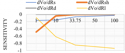
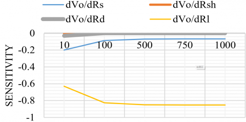
Figure 3 depicts the sensitivity of output voltage with variations in the series resistance, shunt resistance, diode resistance, and load resistance.
It can be seen that the sensitivity values are largely constant with a wide range of perturbations in the PV cell parameters around nominal values evaluated for optimal output power design.
(a) Series resistance variation
(b) Shunt resistance variation
(c) Diode resistance variation
(d) Load resistance variation
Figure 3. Output voltage sensitivities with variations in (a) Rs, (b) Rsh, (c) RDiode, (d) Rl
An adjoint circuit method based on Tellegen’s theorem has been successfully formulated and implemented to evaluate the output voltage sensitivity of PV solar cell with respect to four different circuit parameters that are considered: series, shunt, diode and load resistances. The results have been validated with less than 1% error using the gradient of the function with respect to variations in each parameter according to the approximate CFD method. It has been found the calculated sensitivities are largely constant over a wide range of variations in the 4 parameters around nominal values estimated around the optimal output power V-I characteristic point. The sensitivity is negative for the series resistance and positive for other resistances. The load resistance sensitivity is the largest compared to other parameters. With this sensitivity study, sensitivity of other types of renewable energy system can be used such as wind energy turbines. the performance of PV can be improved by enhancing the manufacturing processes used for them.
|
Isc |
Short circuit current |
|
Voc |
Open circuit voltage |
|
v,i |
Instantaneous voltage and current |
|
Vo |
Output voltage |
|
f |
Objection function |
|
VRl |
Voltage across load resistance |
|
VRs |
Voltage across load resistance |
|
VRsh |
Voltage across shunt resistance |
|
VRth |
Voltage across Thevenin’s resistance |
|
IRl |
Current across load resistance |
|
IRs |
Current across load resistance |
|
IRsh |
Current across shunt resistance |
|
IRth |
Current voltage across Thevenin’s resistance |
|
Y,A,M,Z |
Circuit linear equations matrices |
|
Ia, Ib |
Sub-branch matrix currents |
|
Va, Vb |
Sub-branch matrix voltages |
|
Rs |
Series resistance |
|
Rsh |
Shunt resistance |
|
Rth |
Thevenin’s resistance |
|
Rl |
Load resistance |
|
x |
Variable |
|
Greek symbols |
|
|
[]~ |
Adjoint value symbol |
[1] Saltelli, A., Chan, K., Scott, M. (2000). Sensitivity Analysis. Probability and Statistics Series. John and Wiley & Sons, New York.
[2] Bakr, M. (2013). Nonlinear Optimization in Electrical Engineering with Applications in MATLAB. London: Institution of Engineering and Technology.
[3] Gupta, N., Garg, R., Kumar, P. (2017). Sensitivity and reliability models of a PV system connected to grid. Renewable and Sustainable Energy Reviews, 69: 188-196. https://doi.org/10.1016/j.rser.2016.11.031
[4] Li, J., Ahsanullah, D., Gao, Z., Rohrer, R. (2023). Circuit theory of time domain adjoint sensitivity. IEEE Transactions on Computer-Aided Design of Integrated Circuits and Systems, 42(7): 2303-2316. https://doi.org/10.1109/TCAD.2023.3260163
[5] Director, S., Rohrer, R. (1969). The generalized adjoint network and network sensitivities. IEEE Transactions on Circuit Theory, 16(3): 318-323. https://doi.org/10.1109/TCT.1969.1082965
[6] Bakr, M.H., Nikolova, N.K. (2004). An adjoint variable method for time-domain TLM with wide-band Johns matrix boundaries. IEEE Transactions on Microwave Theory and Techniques, 52(2): 678-685. https://doi.org/10.1109/TMTT.2003.822034
[7] Georgieva, N.K., Glavic, S., Bakr, M.H., Bandler, J.W. (2002). Feasible adjoint sensitivity technique for EM design optimization. IEEE Transactions on Microwave Theory and Techniques, 50(12): 2751-2758. https://doi.org/10.1109/MWSYM.2002.1011791
[8] Ahmed, O.S., Bakr, M.H., Li, X., Nomura, T. (2012). A time-domain adjoint variable method for materials with dispersive constitutive parameters. IEEE Transactions on Microwave Theory and Techniques, 60(10): 2959-2971. https://doi.org/10.1109/TMTT.2012.2207736
[9] Rashel, M.R., Albino, A., Goncalves, T., Tlemcani, M. (2016). Sensitivity analysis of parameters of a photovoltaic cell under different conditions. In 2016 10th International Conference on Software, Knowledge, Information Management & Applications (SKIMA), Chengdu, China, pp. 333-337. https://doi.org/10.1109/SKIMA.2016.7916242
[10] Chen, S., Farkoush, S.G., Leto, S. (2020). Photovoltaic cells parameters extraction using variables reduction and improved shark optimization technique. International Journal of Hydrogen Energy, 45(16): 10059-10069. https://doi.org/10.1016/j.ijhydene.2020.01.236
[11] Chandran, B.P., Selvakumar, A.I., Let, G.S., Sathiyan, S.P. (2021). Optimal model parameter estimation of solar and fuel cells using improved estimation of distribution algorithm. Ain Shams Engineering Journal, 12(2): 1693-1700. https://doi.org/10.1016/j.asej.2020.07.034
[12] Antoniadis, A., Lambert-Lacroix, S., Poggi, J.M. (2021). Random forests for global sensitivity analysis: A selective review. Reliability Engineering & System Safety, 206: 107312. https://doi.org/10.1016/j.ress.2020.107312
[13] Zhang, F., Han, C., Wu, M., Hou, X., Wang, X., Li, B. (2022). Global sensitivity analysis of photovoltaic cell parameters based on credibility variance. Energy Reports, 8: 7582-7588. https://doi.org/10.1016/j.egyr.2022.05.280
[14] Zhu, X.G., Fu, Z.H., Long, X.M. (2011). Sensitivity analysis and more accurate solution of photovoltaic solar cell parameters. Solar Energy, 85(2): 393-403. https://doi.org/10.1016/j.solener.2010.10.022
[15] Praene, J.P., Marc, O., Ennamiri, H., Rakotondramiarana, H.T. (2014). Sensitivity analysis to optimize a solar absorption cooling system. Energy Procedia, 57: 2636-2645. https://doi.org/10.1016/j.egypro.2014.10.275
[16] Kalliojärvi-Viljakainen, H., Lappalainen, K., Valkealahti, S. (2022). A novel procedure for identifying the parameters of the single-diode model and the operating conditions of a photovoltaic module from measured current–voltage curves. Energy Reports, 8: 4633-4640. https://doi.org/10.1016/j.egyr.2022.03.141
[17] Shaik, F., Lingala, S.S. Veeraboina, P. (2023). Effect of various parameters on the performance of solar PV power plant: A review and the experimental study. Sustainable Energy Research, 10: 6. https://doi.org/10.1186/s40807-023-00076-x
[18] Mesbahi, O., Tlemcani M., Janeiro, F.M., Hajjaji, A., Kandoussi, K. (2021). Sensitivity analysis of a new approach to photovoltaic parameters extraction based on the total least squares method. Metrology and Measurement Systems, 28(4): 751-765. https://doi.org/10.24425/mms.2021.137707
[19] Chowdhury, G., Kladas, A., Herteleer, B., Cappelle, J., Catthoor, F. (2021). Sensitivity analysis of the state of the art silicon photovoltaic temperature estimation methods over different time resolution. In IEEE 48th Photovoltaic Specialist Conference (PVSC), Fort Lauderdale, USA, pp. 1340-1343. https://doi.org/10.1109/PVSC43889.2021.9519068
[20] Ziar, H., Karegar, H.K. (2013). Sensitivity analysis of solar photovoltaic modules to environmental factors through new definitions of formula. Journal of Renewable and Sustainable Energy, 5(5): 053108. https://doi.org/10.1063/1.4821292
[21] Verma, V., Mahajan, P., Garg, R. (2021). Sensitivity analysis of solar PV system for different PV array configurations. Communications in Computer and Information Science. In Data Science and Computational Intelligence, pp. 292-403. https://doi.org/10.1007/978-3-030-91244-4_31