Mahdi Abed Atiyah![]() | Lwaa Faisal Abdulameer*
| Lwaa Faisal Abdulameer*![]()
© 2025 The authors. This article is published by IIETA and is licensed under the CC BY 4.0 license (http://creativecommons.org/licenses/by/4.0/).
OPEN ACCESS
Recently, given the increasing need for low-latency, high-efficiency communication in 5G networks, our study addresses key limitations by introducing dual-hop free-space optical (FSO) communication between two devices, it emerges as a promising solution to meet these requirements by utilizing line-of-sight (LOS), the study considers scenarios where devices are distant or degrades due atmospheric turbulence (AT). An optical relay device (ORD) is required to create a dual-hop FSO link. a beam-shaping technique is being employed to maximize the overall signal-to-noise ratio (SNR) at the ORD to focus the beams more tightly towards and minimizing interferences between individual beams. Space time line code (STLC) and space time block code (STBC) are two encoding techniques that can save processing time and increase reliability transmissions at of system. The STLC and STBC encoding use at first and second hop respectively. Also, orthogonality and quasi-orthogonality is used for STLC-STBC to enable the highest possible system capacity and the least processing complexity in ORD. The results from the simulation showed that channel capacity increases with beam-shaping at ORD, especially between ORD and D2, and use OSTLC-OSTBC achieving minimum processing significantly increases communication reliability, and increases system capacity, especially in using 8×8 MIMO instead of 4×4 MIMO.
beamforming, device-to-device, free-space optical (FSO), relay device, space time block code (STBC), space time line code (STLC)
Recently, fifth-generation and beyond (5Gb) technology has exhibited robust capabilities, including high bandwidth, speed, low power consumption, and support for virtual reality. yet it faces challenges in meeting the escalating demands for connectivity [1]. Optical communication, owing to its cost-effectiveness and high-speed connectivity, has gained increasing significance over the past few decade [2]. D2D is a top contender to satisfy the 5Gb needs. To meet high data and transmission speeds and guarantee minimal power consumption, the connectivity of D2D is direct connections rathan needing a base station (BS) for this requirement [3]. However, to fully harness the potential of FSO technology in meeting 5Gb requirements, it is imperative to address fundamental limitations. These limitations include the impact of AT, restricted support for non-LOS (NLOS) communication, and limited mobile connectivity [4].
FSO technology covers Near Infrared (NIR), Visible Light (VL), and Ultraviolet (UV) bands, offering immunity to multi-path fading. In contrast, Radio-Frequency (RF) connections are susceptible to such fading. Optical components in FSO systems are cost-effective, smaller, lighter, and more energy-efficient than RF components [5]. FSO is an optical communication advancement transmitting light in free space, acting as a fiber optic link without the installation time, licenses, and high costs associated with traditional fiber optic systems. FSO systems find applications in last-mile access, backup links, and extending fiber networks quickly and easily. FSO is poised to address bandwidth and rate bottlenecks in 5G networks, laying the foundation for faster, smarter, and more reliable future communication services [6]. Optical communication system networks are achieving a multi of requirements of 5Gb that leads to big translation amounts of data [7].
The diversity technique can enhance the data transmission in the FOS link, improving the spectrum efficiency of wireless optical communication at a high rate [8]. The distances between the receiver and the transmitter are greatly affected by the performance of the link outage or degradation [9].
An RD is positioned to ensure far connectivity of D2D communication distance. Whereas the link survival reliability of far-distance FSO communications must be carefully measured. For achieving energy-efficient and dependable communication connectivity, a multi-hop system has this led to attracted the of researchers [10-12].
Our study specifically focuses on overcoming the challenge of NLOS communication in urban environments by Place a relay between the two devices as a communication link to reduce the distance between them and increase the reliability of the link, due FSO systems are susceptible to interference between sender and receiver, such as a soaring bird and a tree, because they rely on LOS connectivity. Furthermore, it is sensitive to weather conditions; the performance of FSO decreases considerably in strong AT, such as fog and snow; these factors diminish the performance of FSO.
A transmission algorithm must be used in this relay-aided D2D connection that uses the least amount of ORD processing, energy, and time. Decoding and full Channel State Information (CSI) estimates in ORD take longer, greatly impacting the signal's efficiency. To reduce ORD processing and time resources, we propose a suitable technique represented by STLC and STBC. For this, when receiving signals at ORD is not required CSI. Also, at ORD is no requirement of CSI to send signals with STLC and STBC encoding respectively. The attenuation of channel increased due as the weather conditions on the laser beam affects [13]. In D2D communication, relay nodes have been used to reduce link distance and increase reliability. High-performance connectivity is achieved by combining common beamforming and diversity technologies to improve the network bandwidth of 5Gb [14, 15].
It is necessary form a that shaping optical signals in the same direction to working together as single source at the same wavelength and phase by beamforming in ORD. This results in a longer and more targeted stream. The beam is getting as the number of radiating elements increases. in 5G, digital beamforming is most typically employed in the baseband processor nowadays. Beamforming and Multiple-Input Multiple-Output (MIMO) work together to deliver 5G’s capacity throughput and connection reliability. To focus the beam of signals in tightly towards point at receiver can be beamforming technique, this leads to concentrate beams of multi signal more precisely. The beamforming is achieving high connection density and reducing interference between individual beams [16]. Beamforming improves signal quality and reduces processing time by focusing on relevant signals. also, by suppressing interference, the system can focus on processing the desired signals, reducing the computational load and enhancing processing efficiency.
The important objectives that will have been achieved in this paper:
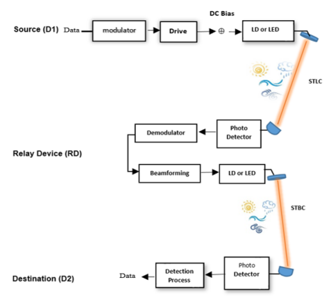
Figure 1. Environmental of FSO dual-hop with ORD
The research provides a good algorithm depending on STLC and STBC to ensure minimal processing and reliable transmission, and the validation of analytical results by MATLAB simulation results.
In D2D communication, relay nodes have been used to reduce link distance and increase reliability. High-performance connectivity is achieved by combining common beamforming and MIMO technologies to improve the network bandwidth of 5G [14].
Space-Time Code (STC) provides spatial diversity to mitigate multipath fading, decreasing the Bit Error Rate (BER), and enhancing the capacity and reliability of communication. However, STC requires full Channel State Information (CSI) at the receiver (ORD) from the sender, leading to potential delays [17].
For achieved high data rate/ capacity, which Space Time Trellis Code Modulation (STTCM) is been used to improve transition signal and power efficiency for full diversity [18]. On the other hand, STTCM generates computational complexity in decoding symbols. This does not require additional processing time for the received data, which contributes to energy drainage [18].
Space Frequency Line Code (SFLC) achieves marginally inferior BER performance compared to STLC for multiple paths, but the efficacy of BER increases with more outputs and inputs. STBC-STLC with orthogonality and quasi-orthogonality, while maintaining competitive BER performance, may offer advantages in terms of reduced delays in transmission compared to SFLC [19].
STLC Spatial Modulation (STLC-SM) requires partial CSI during decoding, reducing complexity, but requires full CSI during transmission. This generates some delay. STBC-STLC may offer reduced complexity in decoding while maintaining similar or improved BER performance compared to STLC-SM [20].
Double STLC (DSTLC) transmits two STLC streams simultaneously, improving spatial diversity and increasing system capacity. However, DSTLC requires more delay when decoding symbols at ORD compared to STLC. DSTLC shows better data rate performance compared to STBC, but it depends on high SNR [21].
Differential SM-STBC increases diversity gain without the need for CSI at the transmitters. Differential SM-STBC optimizes the system in terms of reducing BER, but CSI is not required during decoding at the receiver [22].
Many of the techniques discussed have certain limitations. The primary issue is the high computational complexity involved in encoding and the challenges in decoding. Additionally, some methods require CSI during transmission or reception, which can introduce processing delays and increase power consumption. As a result, these techniques will be excluded. The RD should not rely on CSI estimation, and there should be no decoding required when transmitting or receiving signals in the RD.
The selection of STLC-STBC technologies and associated developments as transfer technologies is central to achieving the objectives of our paper. Here, it is proposed to utilize a suitable algorithm, as represented by STLC and STBC, to minimize processing and time resources at the RD. This aims to eliminate the necessity for CSI to be present when receiving symbols encoded for STLC technology in the RD at the first hop. Additionally, there is no need for CSI when sending symbols encoded by STBC technology at the second hop. Therefore, orthogonality in STLC and STBC contributes to minimal processing. It is proposed by Dimas et al. [23] that STLC be used to achieve full rate by utilizing its orthogonality and quasi-orthogonality. It has been sufficient to achieve a full transmission rate instead of other techniques.
Orthogonality in STLC and STBC helps achieve low latency by minimizing processing, but it does not affect energy usage [24]. In this study, it aims to enhance the energy efficiency of processing signal at ORD by utilized QOSTLC-QOSTBC techniques. it introduces greater symbol overlap. To reduce this, we propose integrating MIMO and beamforming within the ORD and achieving optimize the overall SNR. Additionally, in the proposed system, the beamforming technique maximizes the total SNR ratio in the dual-hop FSO system [25], enhancing the effectiveness of the link between RD and D2. Since STBC encoding does not need to provide CSI, less time and energy are used. Because they don't require CSI on both communication sides, STLC and STBC were chosen as sensible options. Compared to other diversity methods, their practical deployment is extremely simple [26].
The QOSTLC-QOSTBC combination maintains the single coding rate while enhancing BER performance. It approximates OSTBC/OSTLC in terms of transmission latency and quasi-OSTBC/OSTLC in terms of BER values. So far, with recent optical wireless transmission techniques, a relay-based FSO system has yet to be described to the level that meets what we aim to achieve in this paper. Therefore, the focus in this paper is exclusively on OSTLC and OSTBC encoding to meet our objectives, utilizing these techniques will have been minimizing processing in ORD. This is related to the above techniques in addition to adopting some techniques such as OSTLC-OSTBC and QOSTLC-QOSTBC. Furthermore, by increasing diversity through MIMO and beamforming technology, we aim to enhance channel gain and the reliability of data transmission to the maximum extent achievable.
In our proposed system, we consider two devices that are not linked to a BS and are connected to each other over a wireless channel at a significant distance apart. To reduce the challenges of this limitation, a RD is considered between two devices in a dual-hop manner. The system is set up such that the first device has (m) transmitting LEDs, and the second device has (n) PDs. The two devices communicate with each other through an optical RD that has (k) PDs. This results in a D1-RD transmission at the first hop, and an RD-D2 transmission at the second hop thanks to a (j) transmitter of LEDs. The two hops (RD-D1 and D2-RD) are investigated under independent channel circumstances. The primary goal is to use the two coding techniques; STBC at the second hop and STLC at the first hop to achieve low time/energy processing at the RD. A zero mean and variance σ2 of Additive White Gaussian Noise (AWGN) is used to model as shown in Figure 2.
The information voltage signal from the On-Off Keying (OOK) modulation is converted into modulation current appropriate for an LED source by the driving circuit in the block diagram. After that, the PDs will receive the signal at RD. The ORD uses Maximum Ratio Combining (MRC) to combine all the received signals, which optimizes the SNR at the ORD. As a result, at stage (Beamforming), the incoming signals multiply the beamforming factor (W). The signal is then retransmitted to the second device, which has n PDs, as a block of symbols loaded in j LEDs.
Figure 2. Proposed system model
3.1 STLC-STBC in the proposed dual-hop FSO system
An STLC and STBC Techniques are a symbols encoding techniques used to enhance the performance of wireless communication systems. Information symbols are encoded using the multiple channel gains (space) and are transmitted at time slots (time). Given that the coded symbols are transmitted sequentially through a multi transmit antenna, they are a line-shaped of STLC compared to the block shape of STBC. The CSI is not available; these devices will experience challenging performance degradation [27]. An OSTBC - QOSTBC do not support both full diversity and full code rate simultaneously for more than two transmit antennas. An QOSTBC is enhance rates but this leads to Inter-Symbol Interference (ISI) by using a greater number of MIMO can be reduced effect of ISI [28]. On the other hand, the orthogonality in STLC-STBC reduces computational requirements, leading to lower latency but does not impact energy consumption. Symbol transmission is handled by a single relay device with low complexity and minimal processing requirements.
In D2D aided-relay node communication, it is important to utilized a transmission technique that consumes the least amount of processing resources at ORD. Because decoding and full CSI of symbols at ORD result in long time of processing and can have a substantial influence on the energy efficiency of the optical signal. We employ STLC-STBC techniques in mitigate of this challenge. similar to STLC-STBC, OSTLC-OSTBC provides diversity gain and reliability in fading channels, contributing to reduced latency by simplifying decoding processes, also, QOSTBC, with its compromise between orthogonality and complexity, can contribute to lower decoding complexity, potentially reducing processing time.
3.2 Transmission model for the first hop (D1-ORD transmission) by using OSTLC
The modulation scheme used for the first hop from device 1 is OOK, where there is no intensity during transmission as 0 , and an optical intensity is transmitted when 1 occurs (i.e., $X_{D_1-O R D} \in\{0,1\}$). For (M) LEDs from $D_1$ (i.e., $X \in R^{M \times 1}$). The transmitted signal is denoted by:
$\overline{\mathrm{X}}_{\mathrm{D} 1-\mathrm{ORD}}=\sqrt{\frac{\mathrm{P}_{\mathrm{T}}}{\mathrm{M}}} \sum_{\mathrm{K}=0}^3 \mathrm{x}(\mathrm{k})$ (1)
where, PT denotes the transmitted power and $\mathrm{X}_{\mathrm{D}_1 \text {-ORD }} \in$ $\mathrm{R}^{\mathrm{M} \times 1}$. Let the space-time matrix be represented by the following when there are four LEDs at ORD ORD:
$\mathrm{x}=\left[\begin{array}{cccc}\mathrm{x}_1 & \mathrm{x}_2 & \mathrm{x}_3 & \mathrm{x}_4 \\ \mathrm{x}_2 & -\mathrm{x}_1{ }^* & \mathrm{x}_4{ }^* & -\mathrm{x}_3{ }^* \\ \mathrm{x}_3 & -\mathrm{x}_4 & -\mathrm{x}_1 & \mathrm{x}_2 \\ \mathrm{x}_4 & \mathrm{x}_3{ }^* & -\mathrm{x}_2 & -\mathrm{x}_1{ }^*\end{array}\right]$ (2)
Then the k-th receiving PDs' indication of the received signal at ORD for the first hop is:
$\mathrm{Y}_{\mathrm{D}_1-\mathrm{ORD}}(\mathrm{t})=\mathrm{R} \sum_{\mathrm{k}=0}^3 \sqrt{\frac{\mathrm{P}_{\mathrm{T}}}{\mathrm{M}^2}} \mathrm{H}_{\mathrm{ORD}-\mathrm{D}_1} \mathrm{X}_{\mathrm{D}_1-\mathrm{ORD}}+\mathrm{N}_{\mathrm{k}}$ (3)
The summation in Eq. (3), where, k is limited from 0 to 3 because we assume four PDs at ORD, R is PDs responsivity, $\mathrm{H}_{\mathrm{ORD}-\mathrm{D}_1}$ is the channel matrix between LEDs at D1 and PDs at ORD, and each element in the matrix hK,M denotes the channel coefficient between k-th PDs of ORD and M-th LEDs of D1 such that:
$\mathrm{H}_{\mathrm{ORD}-\mathrm{D}_1}=\left[\begin{array}{cccc}\mathrm{h}_{1.1} & \mathrm{~h}_{1.2} & \cdots & \mathrm{~h}_{1 . \mathrm{M}} \\ \mathrm{h}_{2.1} & \mathrm{~h}_{2.2} & \cdots & \mathrm{~h}_{2 . \mathrm{M}} \\ \vdots & \vdots & \ddots & \vdots \\ \mathrm{h}_{\mathrm{K} .1} & \cdots & \cdots & \mathrm{~h}_{\mathrm{K} . \mathrm{M}}\end{array}\right]$ (4)
Consider Fisher-Snedecor $\mathscr{F}$ models each component of the channel matrix $h_{\text {K,M}}$ to simulate the turbulence of the FSO link.
$h_{K . M}=h^{P L} h^{A T} h^{P E}$ (5)
where, hPL, hAT and hPE are the deterministic propagation loss, AT attenuation, and pointing error, respectively. A PDF of AT can be represented for both links as [29]:
$f_{h^{A T}}(x)=\frac{\Gamma(\alpha+\beta) \alpha^\alpha(\beta-1)^\beta x^{\alpha-1}}{\Gamma(\alpha) \Gamma(\beta)(\alpha x+\beta-1)^{\alpha+\beta}}$ (6)
where, α and β are two variables that are the internal and external measures of disturbance, respectively. as they have an important role in affecting the optical propagation properties of the link, where [29]:
$\alpha=\frac{1}{\exp \left(\sigma_{\text {Inn }}^2\right)-1}$ (7)
$\beta=\frac{1}{\exp \left(\sigma_{\operatorname{Inm}}^2\right)-1}+2$ (8)
where, $\sigma_{\mathrm{In} n}^2$ and $\sigma_{\mathrm{In} m}^2$ are the small-scale and large-scale logirradiance variances, respectively, where $\sigma_{I n s}^2$ can be expressed as:
$\sigma_{\mathrm{Inn}}^2=\frac{0.51 \delta_{\mathrm{SP}}^2\left(1+0.69 \delta_{\mathrm{SP}}^{\frac{12}{5}}\right)^{-5 / 6}}{1+0.90 \mathrm{~d}^2\left(\frac{\sigma}{\delta_{\mathrm{SP}}}\right)^{12 / 5}+0.62 \mathrm{~d}^2 \sigma^{12 / 5}}$ (9)
where, $\delta_{\mathrm{SP}^2}$ is the spherical scintillation index (SSI) of the FSO link [29]. $\sigma^2$ represents the strength of irradiance fluctuations, and d is the equivalent aperture diameter.
At the first-time interval [0, Ts], the receiving symbol sequences are:
$\begin{gathered}\mathrm{r}_{\mathrm{D} 1-\mathrm{ORD}}(1)=\mathrm{R} \frac{1}{\sqrt{\sum_{\mathrm{M}=1}^4 \sum_{\mathrm{k}=1}^4\left[\mathrm{~h}_{\mathrm{oRD}-\mathrm{D} 1}\right]^2}} \sum_{\mathrm{i}=1}^{\mathrm{F}} \sqrt{\frac{\mathrm{P}_{\mathrm{T}}}{4}}\left[\mathrm{~h}_{1.1} \mathrm{x}_1+\right. \left.\mathrm{h}_{1.2} \mathrm{x}_2+\mathrm{h}_{1.3} \mathrm{x}_3+\mathrm{h}_{1.4} \mathrm{x}_4\right] \mathrm{f}_{\mathrm{i}}+\mathrm{N}_1\end{gathered}$ (10)
At the second time interval [Ts, 2Ts]:
$\begin{gathered}\mathrm{r}_{\mathrm{ORD}}(2)=\mathrm{R} \frac{1}{\sqrt{\sum_{\mathrm{M}=1}^4 \sum_{\mathrm{k}=1}^4\left[\mathrm{~h}_{\mathrm{ORD}-\mathrm{D} 1}\right]^2}} \sum_{\mathrm{i}=1}^{\mathrm{F}} \sqrt{\frac{\mathrm{P}_{\mathrm{T}}}{4}}\left[\mathrm{~h}_{2.1} \mathrm{x}_2-\right. \left.\mathrm{h}_{2.2} \mathrm{x}_1{ }^*-\mathrm{h}_{2.3} \mathrm{x}_4+\mathrm{h}_{2.4} \mathrm{x}_3{ }^*\right] \mathrm{f}_{\mathrm{i}}+\mathrm{N}_2\end{gathered}$ (11)
At the third time interval [2Ts, 3Ts],
$\begin{gathered}r_{\text{ORD}}(3) = R \frac{1}{\sqrt{\sum_{M=1}^4 \sum_{k=1}^4 \left[h_{\text{ORD-D}_1}\right]^2}} \sum_{i=1}^{F} \sqrt{\frac{P_T}{4}} \left[ h_{3.1} x_3 + h_{3.2} x_4^* - h_{3.3} x_1 - h_{3.4} x_2 \right] f_i + N_3\end{gathered}$ (12)
At the fourth time interval [3Ts, 4Ts]:
$\begin{gathered}\mathrm{r}_{\mathrm{ORD}}(4)=\mathrm{R} \frac{1}{\sqrt{\sum_{\mathrm{M}=1}^4 \sum_{\mathrm{k}=1}^4\left[\mathrm{~h}_{\mathrm{ORD}-\mathrm{D} 1}\right]^2}} \sum_{\mathrm{i}=1}^{\mathrm{F}} \sqrt{\frac{\mathrm{P}_{\mathrm{T}}}{4}}\left[\mathrm{~h}_{4.1} \mathrm{x}_4-\right. \left.\mathrm{h}_{4.2} \mathrm{x}_3{ }^*+\mathrm{h}_{4.3} \mathrm{x}_2-\mathrm{h}_{4.4} \mathrm{x}_1{ }^*\right] \mathrm{f}_{\mathrm{i}}+\mathrm{N}_4\end{gathered}$ (13)
The effective channel gain at ORD is expressed as:
$\sqrt{\sum_{\mathrm{m}=1}^4 \sum_{\mathrm{k}=1}^4\left\lceil\mathrm{~h}_{\mathrm{ORD}-\mathrm{D} 1}\right\rceil^2}$ (14)
where, $\mathrm{N}_1 \mathrm{~N}_2 \mathrm{~N}_3$ and $\mathrm{N}_4$ are the AWGN vectors at each PD at ORD. Each AWGN is with mean zero and variance $\sigma_N^2$. Four LEDs exist at $D_1$ and four PDs exist at ORD. Where $f_i \in$ $\mathrm{R}^{\mathrm{M} \times 1}$ is the beamforming matrix multiplied by the data symbols of the transmitted signal vector at $D_1$. Because $D_{1-}$ ORD uses STLC. Where ORD did not require the CSI and did not perform any decoding processing. As a result, the amount of delay and power consumption will be reduced of system. ORD merely needs to combine all the received on the $\mathrm{X}_{\mathrm{D}_1-\text { ORD }}$ matrix in Eq. (2), such that:
$\overline{\mathrm{x}}_1=\mathrm{r}_{\mathrm{ORD}}(1)+\mathrm{r}_{\mathrm{ORD}}(2)+\mathrm{r}_{\mathrm{ORD}}(3)+\mathrm{r}_{\mathrm{ORD}}(4)$ (15)
$\overline{\mathrm{x}}_2=\mathrm{r}_{\mathrm{ORD}}(2)-\mathrm{r}_{\mathrm{ORD}}(1)^*+\mathrm{r}_{\mathrm{ORD}}(4)^*-\mathrm{r}_{\mathrm{ORD}}(3)^*$ (16)
$\overline{\mathrm{x}}_3=\mathrm{r}_{\mathrm{ORD}}(3)-\mathrm{r}_{\mathrm{ORD}}(4)-\mathrm{r}_{\mathrm{ORD}}(1)+\mathrm{r}_{\mathrm{ORD}}(2)$ (17)
$\overline{\mathrm{x}}_4=\mathrm{r}_{\mathrm{ORD}}(4)+\mathrm{r}_{\mathrm{ORD}}(3)^*+\mathrm{r}_{\mathrm{ORD}}(2)+\mathrm{r}_{\mathrm{ORD}}(1)^*$ (18)
These estimated symbols can be rewritten as:
$\begin{gathered}\overline{\mathrm{x}}_1=\operatorname{sign}\left\{\sqrt{\left|\mathrm{h}_{1.1}+\mathrm{h}_{1.2}+\mathrm{h}_{1.3}+\mathrm{h}_{1.4}\right|^2 \mathrm{x}_1}\left(\mathrm{~h}_{1.1}\right.\right. \left.\left.+\mathrm{h}_{1.2}+\mathrm{h}_{1.3}+\mathrm{h}_{1.4}\right) \mathrm{N}_1\right\}\end{gathered}$ (19)
$\begin{gathered}\overline{\mathrm{x}}_2=\operatorname{sign}\left\{\sqrt{\left|\mathrm{h}_{2.1}+\mathrm{h}_{2.2}+\mathrm{h}_{2.3}+\mathrm{h}_{2.4}\right|^2 \mathrm{x}_2}\left(\mathrm{~h}_{2.1}\right.\right. \left.\left.+\mathrm{h}_{2.2}+\mathrm{h}_{2.3}+\mathrm{h}_{2.4}\right) \mathrm{N}_2\right\}\end{gathered}$ (20)
$\begin{gathered}\overline{\mathrm{x}}_3=\operatorname{sign}\left\{\sqrt{\left|\mathrm{h}_{3.1}+\mathrm{h}_{3.2}+\mathrm{h}_{3.3}+\mathrm{h}_{3.4}\right|^2 \mathrm{x}_3}\left(\mathrm{~h}_{3.1}\right.\right. \left.\left.+\mathrm{h}_{3.2}+\mathrm{h}_{3.3}+\mathrm{h}_{3.4}\right) \mathrm{N}_3\right\}\end{gathered}$ (21)
$\begin{gathered}\overline{\mathrm{x}}_4=\operatorname{sign}\left\{\sqrt{\left|\mathrm{h}_{4.1}+\mathrm{h}_{4.2}+\mathrm{h}_{4.3}+\mathrm{h}_{4.4}\right|^2 \mathrm{x}_4}\left(\mathrm{~h}_{4.1}\right.\right. \left.\left.+\mathrm{h}_{4.2}+\mathrm{h}_{4.3}+\mathrm{h}_{4.4}\right) \mathrm{N}_4\right\}\end{gathered}$ (22)
However, the MRC technique maximizes SNR at ORD, is used to combine all of the received signals at any receiving device in our system (ORD and D2). Therefore, the beamforming factor (W) is multiplied by the received signals as follows:
$\begin{gathered}\mathrm{W}_1{ }^* \mathrm{r}_{\mathrm{ORD}}(1)+\mathrm{W}_2{ }^* \mathrm{r}_{\mathrm{ORD}}(2)+\mathrm{W}_3{ }^* \mathrm{r}_{\mathrm{ORD}}(3) \left.+\mathrm{W}_4{ }^* \mathrm{r}_{\mathrm{ORD}}(4)\right]\end{gathered}$ (23)
The above equation can be rewritten as:
$\left[\mathrm{W}_1^* \mathrm{~W}_2^* \mathrm{~W}_3^* \mathrm{~W}_4^*\right]\left[\begin{array}{l}\mathrm{r}_{\mathrm{ORD}}(1) \\ \mathrm{r}_{\mathrm{ORD}}(2) \\ \mathrm{r}_{\mathrm{ORD}}(3) \\ \mathrm{r}_{\mathrm{ORD}}(4)\end{array}\right]=\overline{\mathrm{W}}_{\mathrm{M}}^H \overline{\mathrm{r}}_{\mathrm{ORD} . \mathrm{j}}$ (24)
where, H is denoted to the Hermitian matrix for W.
Then, the output of MRC is denoted by:
$\overline{\mathrm{W}}^H{ }_1 \sum_{\mathrm{i}=1}^{\mathrm{F}} \sqrt{\frac{\mathrm{P}_{\mathrm{T}}}{4}}\left[\mathrm{~h}_{1.1} \mathrm{x}_1+\mathrm{h}_{1.2} \mathrm{x}_2+\mathrm{h}_{1.3} \mathrm{x}_3+\mathrm{h}_{1.4} \mathrm{x}_4\right] \mathrm{f}_{\mathrm{i}}+\overline{\mathrm{W}}^H{ }_1 \mathrm{~N}_1$ (25)
$\overline{\mathrm{W}}^H{ }_2 \sum_{\mathrm{i}=1}^{\mathrm{F}} \sqrt{\frac{\mathrm{P}_{\mathrm{T}}}{4}}\left[\mathrm{~h}_{2.1} \mathrm{x}_2-\mathrm{h}_{2.2} \mathrm{x}_1{ }^*+\mathrm{h}_{2.3} \mathrm{x}_4{ }^*-\mathrm{h}_{2.4} \mathrm{x}_3{ }^*\right] \mathrm{f}_{\mathrm{i}}+\overline{\mathrm{W}}^H{ }_2 \mathrm{~N}_2$ (26)
$\overline{\mathrm{W}}^H{ }_3 \sum_{\mathrm{i}=1}^{\mathrm{F}} \sqrt{\frac{\mathrm{P}_{\mathrm{T}}}{4}}\left[\mathrm{~h}_{3.1} \mathrm{x}_3+\mathrm{h}_{3.2} \mathrm{x}_4+\mathrm{h}_{3.3} \mathrm{x}_1+\mathrm{h}_{3.4} \mathrm{x}_2\right] \mathrm{f}_{\mathrm{i}}+\overline{\mathrm{W}}^H{ }_3 \mathrm{~N}_3$ (27)
$\overline{\mathrm{W}}^H{ }_4 \sum_{\mathrm{i}=1}^{\mathrm{F}} \sqrt{\frac{\mathrm{P}_{\mathrm{T}}}{4}}\left[\mathrm{~h}_{4.1} \mathrm{x}_4+\mathrm{h}_{4.2} \mathrm{x}_3{ }^*-\mathrm{h}_{4.3} \mathrm{x}_2-\mathrm{h}_{1.4} \mathrm{x}_1{ }^*\right] \mathrm{f}_{\mathrm{i}}+\overline{\mathrm{W}}^H{ }_4 \mathrm{~N}_4$ (28)
Full-spatial variety is attained by combining the four received symbols in (the equations above) to decode the STLC symbols, as shown in Figure 3.
Figure 3. A full-spatial-diversity 4×4 STLC system
The SNR for the first hop (D1-ORD) is completed by derivation, however,
$\text{Signal power}=\mathrm{E}\left|\overline{\mathrm{~W}}^H \mathrm{H}\right|^2\left|\mathrm{X}_{\mathrm{D}_1-\mathrm{RD}}\right|^2 \mathrm{E}\left|\overline{\mathrm{~W}}^H \mathrm{H}\right|^2 \mathrm{E}\left|\mathrm{X}_{\mathrm{D}_1-\mathrm{RD}}{ }^H \mathrm{X}_{\mathrm{D}_1-\mathrm{RD}}\right|$ (29)
where, $\mathrm{X}_{\mathrm{D}_1-\mathrm{ORD}}{ }^{\mathrm{H}} \mathrm{X}_{\mathrm{D}_1-\mathrm{ORD}}$ is the covariance matrix of the transmitted symbols.
Signal power $=\left|\bar{W}^H \mathrm{H}\right|^2\left[\begin{array}{l}\mathrm{x}_1 \\ \mathrm{x}_2 \\ \mathrm{x}_3 \\ \mathrm{x}_4\end{array}\right]\left[\mathrm{x}_1{ }^* \mathrm{x}_2{ }^* \mathrm{x}_3{ }^* \mathrm{x}_4{ }^*\right]$ (30)
Signal power $=\left|\bar{W}^H H\right|^2\left[\begin{array}{cccc}\sigma_d^2 & 0 & 0 & 0 \\ 0 & \sigma_d^2 & 0 & 0 \\ 0 & 0 & \sigma_d^2 & 0 \\ 0 & 0 & 0 & \sigma_d^2\end{array}\right]$ (31)
Signal power $=\left|\overline{\mathrm{W}}^H \mathrm{H}\right|^2 \sigma_{\mathrm{d}}^2$ (32)
The noise power has now been finished as follows:
Noise power $=E\left|N_i N_j{ }^*\right|=E\left[\begin{array}{l}N_1 \\ N_2 \\ N_3 \\ N_4\end{array}\right]\left[\mathrm{N}_1{ }^* \mathrm{~N}_2{ }^* \mathrm{~N}_3{ }^* \mathrm{~N}_4{ }^*\right]$ (33)
Noise-power $=\left[\begin{array}{cccc}{\left[\mathrm{N}_1\right]^2} & \mathrm{~N}_1 \mathrm{~N}_2{ }^* & \mathrm{~N}_1 \mathrm{~N}_3{ }^* & \mathrm{~N}_1 \mathrm{~N}_4{ }^* \\ \mathrm{~N}_2 \mathrm{~N}_1{ }^* & {\left[\mathrm{N}_2\right]^2} & \mathrm{~N}_2 \mathrm{~N}_3{ }^* & \mathrm{~N}_2 \mathrm{~N}_4{ }^* \\ \mathrm{~N}_3 \mathrm{~N}_1{ }^* & \mathrm{~N}_3 \mathrm{~N}_2{ }^* & {\left[\mathrm{N}_3\right]^2} & \mathrm{~N}_3 \mathrm{~N}_4{ }^* \\ \mathrm{~N}_4 \mathrm{~N}_1{ }^* & \mathrm{~N}_4 \mathrm{~N}_2{ }^* & \mathrm{~N}_4 \mathrm{~N}_3{ }^* & {\left[\mathrm{N}_4\right]^2}\end{array}\right]$ (34)
where,
$\mathrm{E}\left[\mathrm{N}_{\mathrm{i}} \mathrm{N}_{\mathrm{i}}^*\right]=0, \quad \mathrm{i} \neq \mathrm{j}$ (35)
$\mathrm{E}\left[\left|\mathrm{N}_{\mathrm{i}}\right|^2\right]=\sigma_{\mathrm{N}}^2, \quad \mathrm{i}=\mathrm{j}$ (36)
Hence,
$\mathrm{E}\left[\mathrm{N}_{\mathrm{i}} \mathrm{N}_{\mathrm{j}}^*\right]=\sigma_{\mathrm{N}}^2 \mathrm{I}$ (37)
Then,
Noise power $=\mathrm{E}\left[\overline{\mathrm{W}}^H \mathrm{~N}_{\mathrm{i}}\right]=\overline{\mathrm{W}}^H \sigma_{\mathrm{N}}^2=\sigma_{\mathrm{N}}^2\|\overline{\mathrm{W}}\|^2$ (38)
Hence, the SNR of the first hop is denoted by:
$\operatorname{SNR}_{\mathrm{D}_1-\mathrm{ORD}}=\frac{\left|\overline{\mathrm{W}}^H \mathrm{H}\right| \cdot \sigma_{\mathrm{d}}^2}{\|\overline{\mathrm{~W}}\|^2 \cdot \sigma_{\mathrm{N}}^2}$ (39)
3.3 Transmission model for the second hop (ORD-D2 transmission) by using OSTBC
Let the space-time matrix for the second hop be represented as follows when there are eight LEDs at ORD:
$X_{\text{ORD-D}_2} = \begin{bmatrix} X_1 & X_2 & X_3 & X_4 & X_5 & X_6 & X_7 & X_8 \\ -X_2^* & X_1^* & X_4 & -X_3^* & -X_6^* & X_5^* & X_8 & -X_7^* \\ -X_3^* & -X_4 & X_1^* & X_2^* & -X_7^* & -X_8 & X_5^* & X_6^* \\ -X_4^* & X_3^* & -X_2^* & X_1^* & X_8^* & X_7^* & -X_6^* & X_5^* \\ -X_5^* & -X_6^* & -X_7^* & -X_8^* & X_1 & X_2 & X_3 & X_4 \\ X_6^* & -X_5^* & -X_8 & X_7^* & -X_2^* & X_1^* & -X_4^* & X_3^* \\ X_7^* & X_8 & -X_5^* & -X_6^* & X_3 & X_4^* & -X_1^* & -X_2^* \\ X_8^* & -X_7^* & X_6^* & -X_5^* & -X_4 & -X_3^* & X_2^* & -X_1^* \end{bmatrix}$ (40)
The transmitted signals can be represented by the following using the space-time matrix mentioned above:
$\mathrm{X}_{\mathrm{ORD}-\mathrm{D}_2(1)}=\frac{1}{\sqrt{8}}\left[\mathrm{x}_1 \mathrm{x}_2 \mathrm{x}_3 \mathrm{x}_4 \mathrm{x}_5 \mathrm{x}_6 \mathrm{x}_7 \mathrm{x}_8\right]$ (41)
$\mathrm{X}_{\mathrm{ORD}-\mathrm{D}_2(2)}=\frac{1}{\sqrt{8}}\left[-\mathrm{x}_2{ }^* \mathrm{x}_1{ }^* \mathrm{x}_4-\mathrm{x}_3{ }^*-\mathrm{x}_6{ }^* \mathrm{x}_5{ }^* \mathrm{x}_8-\mathrm{x}_7{ }^*\right]$ (42)
$\mathrm{X}_{\mathrm{ORD}-\mathrm{D}_2(3)}=\frac{1}{\sqrt{8}}\left[-\mathrm{x}_3{ }^*-\mathrm{x}_4 \mathrm{x}_1{ }^* \mathrm{x}_2{ }^*-\mathrm{x}_7{ }^*-\mathrm{x}_8 \mathrm{x}_5{ }{ }^* \mathrm{x}_6{ }^*\right]$ (43)
$\mathrm{X}_{\mathrm{ORD}-\mathrm{D}_2(4)}=\frac{1}{\sqrt{8}}\left[-\mathrm{x}_4{ }^* \mathrm{x}_3{ }^*-\mathrm{x}_2{ }^* \mathrm{x}_1{ }^* \mathrm{x}_8{ }^* \mathrm{x}_7{ }^*-\mathrm{x}_6{ }^* \mathrm{x}_5{ }^*\right]$ (44)
$\mathrm{X}_{\mathrm{ORD}-\mathrm{D}_2(5)}=\frac{1}{\sqrt{8}}\left[-\mathrm{x}_5{ }^*-\mathrm{x}_6{ }^*-\mathrm{x}_7{ }^*-\mathrm{x}_8{ }^* \mathrm{x}_1 \mathrm{x}_2 \mathrm{x}_3 \mathrm{x}_4\right]$ (45)
$\mathrm{X}_{\mathrm{ORD}-\mathrm{D}_2(6)}=\frac{1}{\sqrt{8}}\left[\mathrm{x}_6{ }^*-\mathrm{x}_5{ }^*-\mathrm{x}_8 \mathrm{x}_7{ }^*-\mathrm{x}_2 \mathrm{x}_1^*-\mathrm{x}_4{ }^* \mathrm{x}_3{ }^*\right]$ (46)
$\mathrm{X}_{\mathrm{ORD}-\mathrm{D}_2(7)}=\frac{1}{\sqrt{8}}\left[\mathrm{x}_7{ }^* \mathrm{x}_8-\mathrm{x}_5{ }^*-\mathrm{x}_6{ }^* \mathrm{x}_3 \mathrm{x}_4{ }^*-\mathrm{x}_1{ }^*-\mathrm{x}_2{ }^*\right]$ (47)
$\mathrm{X}_{\mathrm{ORD}-\mathrm{D}_2(8)}=\frac{1}{\sqrt{8}}\left[\mathrm{x}_8{ }^*-\mathrm{x}_7{ }^* \mathrm{x}_6{ }^*-\mathrm{x}_5{ }^*-\mathrm{x}_4-\mathrm{x}_3{ }^* \mathrm{x}_2{ }^*-\mathrm{x}_1{ }^*\right]$ (48)
Each element of matrix Hn, j denotes the channel coefficient between n-th PDs of D2 and j-th LEDs of ORD. Again, the Fisher-Snedecor ℱ model is considered for each component of the channel matrix to simulate the turbulence of the FSO link between ORD and D2.
$H_{\text{ORD-D}_2} =\begin{bmatrix}h_{1.1} & h_{2.1} & h_{3.1} & h_{4.1} & h_{5.1} & h_{6.1} & h_{7.1} & h_{8.1} \\h_{1.2} & -h_{2.3} & h_{3.2} & -h_{4.2} & h_{5.2} & -h_{6.2} & h_{7.2} & -h_{8.2} \\h_{1.3} & -h_{2.3} & -h_{3.3} & h_{4.3} & h_{5.3} & h_{6.3} & h_{7.3} & h_{8.3} \\h_{1.4} & h_{2.4} & -h_{3.4} & -h_{4.4} & h_{5.4} & -h_{6.4} & h_{7.4} & -h_{8.4} \\h_{1.5} & h_{2.5} & h_{4.5} & h_{4.5} & h_{5.5} & h_{6.5} & h_{7.5} & h_{8.5} \\h_{1.6} & -h_{2.6} & h_{3.6} & -h_{4.6} & h_{5.6} & -h_{6.6} & h_{7.6} & -h_{8.6} \\h_{1.7} & -h_{2.7} & -h_{3.7} & h_{4.7} & h_{5.7} & h_{6.7} & h_{7.7} & h_{8.7} \\h_{1.8} & h_{2.8} & -h_{3.8} & -h_{4.8} & h_{5.8} & -h_{6.8} & h_{7.8} & -h_{8.8}\end{bmatrix}$ (49)
The signals that were received are recorded as follows:
$\begin{gathered}\mathrm{r}_{\mathrm{D} 2}(1)=\mathrm{R} \sqrt{\frac{\mathrm{P}_{\mathrm{T}}}{8}}\left[\mathrm{~h}_{1.1} \mathrm{x}_1+\mathrm{h}_{1.2} \mathrm{x}_2+\mathrm{h}_{1.3} \mathrm{x}_3+\right. \left.\mathrm{h}_{1.4} \mathrm{x}_4+\mathrm{h}_{1.5} \mathrm{x}_5+\mathrm{h}_{1.6} \mathrm{x}_6+\mathrm{h}_{1.7} \mathrm{x}_7+\mathrm{h}_{1.8} \mathrm{x}_8\right]+\mathrm{Z}_1\end{gathered}$ (50)
$\begin{gathered}\mathrm{r}_{\mathrm{D} 2}(2)=\mathrm{R} \sqrt{\frac{\mathrm{P}_{\mathrm{T}}}{8}}\left[-\mathrm{h}_{2.1} \mathrm{x}_2{ }^*-\mathrm{h}_{2.2} \mathrm{x}_1{ }^*+\mathrm{h}_{2.3} \mathrm{x}_4+\right. \left.\mathrm{h}_{2.4} \mathrm{x}_3{ }^*-\mathrm{h}_{2.5} \mathrm{x}_6{ }^*-\mathrm{h}_{2.6} \mathrm{x}_5{ }^*+\mathrm{h}_{2.7} \mathrm{x}_8-\mathrm{h}_{2.8} \mathrm{x}_7{ }^*\right]+\mathrm{Z}_2\end{gathered}$ (51)
$\begin{gathered}\mathrm{r}_{\mathrm{D} 2}(3)=\mathrm{R} \sqrt{\frac{\mathrm{p}_{\mathrm{T}}}{8}}\left[-\mathrm{h}_{3.1} \mathrm{x}_3{ }^*-\mathrm{h}_{3.2} \mathrm{x}_4+\mathrm{h}_{3.3} \mathrm{x}_1{ }^*+\right. \left.\mathrm{h}_{3.4} \mathrm{x}_2{ }^*-\mathrm{h}_{3.5} \mathrm{x}_7{ }^*-\mathrm{h}_{3.6} \mathrm{x}_8+\mathrm{h}_{3.7} \mathrm{x}_5{ }^*+\mathrm{h}_{3.8} \mathrm{x}_6{ }^*\right]+\mathrm{Z}_3\end{gathered}$ (52)
$\begin{gathered}\mathrm{r}_{\mathrm{D} 2}(4)=\mathrm{R} \sqrt{\frac{\mathrm{P}_{\mathrm{T}}}{8}}\left[-\mathrm{h}_{4.1} \mathrm{x}_4{ }^*-\mathrm{h}_{4.2} \mathrm{x}_3{ }^*-\mathrm{h}_{4.3} \mathrm{x}_2{ }^*-\right. \left.\mathrm{h}_{4.4} \mathrm{x}_1{ }^*+\mathrm{h}_{4.5} \mathrm{x}_8{ }^*+\mathrm{h}_{4.6} \mathrm{x}_7{ }^*-\mathrm{h}_{4.7} \mathrm{x}_6{ }^*-\mathrm{h}_{4.8} \mathrm{x}_5{ }^*\right]+ \mathrm{Z}_4\end{gathered}$ (53)
$\begin{gathered}\mathrm{r}_{\mathrm{D} 2}(5)=\mathrm{R} \sqrt{\frac{\mathrm{P}_{\mathrm{T}}}{8}}\left[-\mathrm{h}_{5.1} \mathrm{x}_5{ }^*-\mathrm{h}_{5.2} \mathrm{x}_6{ }^*-\right.\mathrm{h}_{5.3} \mathrm{x}_7{ }^*-\mathrm{h}_{5.4} \mathrm{x}_8{ }^*+\mathrm{h}_{5.5} \mathrm{x}_1+\mathrm{h}_{5.6} \mathrm{x}_2+\mathrm{h}_{5.7} \mathrm{x}_3+\left.\mathrm{h}_{5.8} \mathrm{x}_4\right]+\mathrm{Z}_5\end{gathered}$ (54)
$\begin{gathered}r_{D 2}(6)=R \sqrt{\frac{p_T}{8}}\left[h_{6.1} x_6{ }^*+h_{6.2} x_5{ }^*-h_{6.3} x_8-\right. \left.h_{6.4} x_7{ }^*-h_{6.5} x_2-h_{6.6} x_1{ }^*-h_{6.7} x_4{ }^*-h_{6.8} x_3{ }^*\right]+Z_6\end{gathered}$ (55)
$\begin{gathered}\mathrm{r}_{\mathrm{D} 2}(7)=\mathrm{R} \sqrt{\frac{\mathrm{P}_{\mathrm{T}}}{8}}\left[\mathrm{~h}_{7.1} \mathrm{x}_7{ }^*+\mathrm{h}_{7.2} \mathrm{x}_8-\mathrm{h}_{7.3} \mathrm{x}_5{ }^*-\right. \left.\mathrm{h}_{7.4} \mathrm{x}_6{ }^*+\mathrm{h}_{7.5} \mathrm{x}_3+\mathrm{h}_{7.6} \mathrm{x}_4{ }^*-\mathrm{h}_{7.7} \mathrm{x}_1{ }^*-\mathrm{h}_{7.8} \mathrm{x}_2{ }^*\right]+\mathrm{Z}_7\end{gathered}$ (56)
$\begin{gathered}\mathrm{r}_{\mathrm{D} 2}(8)=\mathrm{R} \sqrt{\frac{\mathrm{P}_{\mathrm{T}}}{8}}\left[\mathrm{~h}_{8.1} \mathrm{x}_8{ }^*-\mathrm{h}_{8.2} \mathrm{x}_7{ }^*+\mathrm{h}_{8.3} \mathrm{x}_6{ }^*-\right. \left.\mathrm{h}_{8.4} \mathrm{x}_5{ }^*+\mathrm{h}_{8.5} \mathrm{x}_4-\mathrm{h}_{8.6} \mathrm{x}_3{ }^*+\mathrm{h}_{8.7} \mathrm{x}_2{ }^*-\mathrm{h}_{8.8} \mathrm{x}_1{ }^*\right]+\mathrm{Z}_8\end{gathered}$ (57)
At D2, all received signals are combined using the MRC technique. Consequently, the MRC output can be expressed mathematically as follows:
$\begin{gathered}{\left[\mathrm{W}_1{ }^* \mathrm{r}_{\mathrm{D} 2}(1)+\mathrm{W}_2{ }^* \mathrm{r}_{\mathrm{D} 2}(2)+\mathrm{W}_3{ }^* \mathrm{r}_{\mathrm{D} 2}(3)+\right.} \mathrm{W}_4{ }^* \mathrm{r}_{\mathrm{D} 2}(4)+\mathrm{W}_5{ }^* \mathrm{r}_{\mathrm{D} 2}(5)+\mathrm{W}_6{ }^* \mathrm{r}_{\mathrm{D} 2}(6)+ \left.\mathrm{W}_7{ }^* \mathrm{r}_{\mathrm{D} 2}(7)+\mathrm{W}_8{ }^* \mathrm{r}_{\mathrm{D} 2}(8)\right]\end{gathered}$ (58)
The format shown above can be written as follows:
$\left[\mathrm{W}_1{ }^* \mathrm{~W}_2{ }^* \mathrm{~W}_3{ }^* \mathrm{~W}_4{ }^* \mathrm{~W}_5{ }^* \mathrm{~W}_6{ }^* \mathrm{~W}_7{ }^* \mathrm{~W}_8{ }^*\right]\left[\begin{array}{c}\mathrm{r}_{\mathrm{D} 2}(1) \\ \mathrm{r}_{\mathrm{D} 2}(2) \\ \mathrm{r}_{\mathrm{D} 2}(3) \\ \mathrm{r}_{\mathrm{D} 2}(4) \\ \mathrm{r}_{\mathrm{D} 2}(5) \\ \mathrm{r}_{\mathrm{D} 2}(6) \\ \mathrm{r}_{\mathrm{D} 2}(7) \\ \mathrm{r}_{\mathrm{D} 2}(8)\end{array}\right]=\overline{\mathrm{W}}_{\mathrm{n}}^H \overline{\mathrm{r}}_{\mathrm{D}_2}$ (59)
Now let's identify the signals that were picked up by:
$\overline{\mathrm{r}}_{\mathrm{D} 2}=\mathrm{R} \sqrt{\frac{\mathrm{P}_{\mathrm{T}}}{8}} \sum_{\mathrm{n}=1}^8 \mathrm{X}_{\mathrm{ORD}-\mathrm{D}_2} \mathrm{H}_{\mathrm{ORD}-\mathrm{D}_2-\mathrm{n} . \mathrm{j}}+\mathrm{Z}_{\mathrm{n}}$ (60)
Therefore, the output of MRC is denoted by:
$\overline{\mathrm{W}}^H\left(\mathrm{R} \sqrt{\frac{\mathrm{P}_{\mathrm{T}}}{8}} \sum_{\mathrm{n}=1}^8 \mathrm{X}_{\mathrm{ORD}-\mathrm{D}_2} \mathrm{H}_{\mathrm{ORD}-\mathrm{D}_2-\mathrm{n} . \mathrm{j}}+\mathrm{Z}_{\mathrm{n}}\right)$ (61)
However, the maximized SNR becomes:
$\overline{\mathrm{W}}^H \mathrm{R} \sqrt{\frac{\mathrm{P}_{\mathrm{T}}}{8}} \overline{\mathrm{X}}_{\mathrm{ORD}-\mathrm{D}_2} \mathrm{H}_{\mathrm{ORD}-\mathrm{D}_2-\mathrm{n} . \mathrm{j}}+\overline{\mathrm{W}}^H \mathrm{Z}_{\mathrm{n}}$ (62)
signal power $=\frac{\mathrm{P}_{\mathrm{T}}}{8}\left|\overline{\mathrm{~W}}^H \mathrm{H}_{\mathrm{ORD}-\mathrm{D}_2-\mathrm{n} . \mathrm{j}}\right|^2 \mathrm{R}=\sigma_{\mathrm{ORD}-\mathrm{D}_2}^2 \mathrm{I}$ (63)
The $\sigma_{O R D-\mathrm{D}_2}^2$ represents the transmitted power that is computed according to the following criteria:
$\mathrm{E}\left\{\mathrm{X}_{\mathrm{ORD}-\mathrm{D}_2}\right\}=0$ (64)
$\mathrm{E}\left\{\mathrm{X}^2{ }_{\mathrm{ORD}-\mathrm{D}_2}\right\}=\left[\begin{array}{ccc}\sigma_{\mathrm{ORD}-\mathrm{D}_2}^2 & 0 & 0 \\ 0 & \sigma_{\mathrm{ORD}-\mathrm{D}_2}^2 & 0 \\ 0 & 0 & \sigma_{\mathrm{ORD}-\mathrm{D}_2}^2\end{array}\right]$ (65)
$\mathrm{E}\left\{\mathrm{X}^2{ }_{\mathrm{ORD}-\mathrm{D}_2}\right\}=\sigma_{\mathrm{ORD}-\mathrm{D}_2}^2 \mathrm{I}$ (66)
where,
$\mathrm{X}_{\mathrm{ORD}-\mathrm{D}_2} i \,\,\mathrm{X}_{\mathrm{ORD}-\mathrm{D}_2} j=\sigma_{\mathrm{ORD}-\mathrm{D}_2}^2, \quad$ when $i=j$ (67)
$\mathrm{X}_{\mathrm{ORD}-\mathrm{D}_2} i \,\,\mathrm{X}_{\mathrm{ORD}-\mathrm{D}_2} j=\sigma_{\mathrm{ORD}-\mathrm{D}_2}^2, \quad$ when $i=j$ (68)
As shown below, the noise power can be calculated:
$\mathrm{E}\left\{\overline{\mathrm{W}}^H \mathrm{Z}_{\mathrm{n}}\right\}=0$ (69)
$\begin{aligned}{E}\{|\bar{W}^H Z_n|^2\} &= {E}\{(\bar{W}^H Z_n)(\bar{W}^H Z_n)^H\} \\&= {E}\{\bar{W}^H \bar{W}\} {E}\{Z_n Z_n^H\} \\&= \bar{W}^H \bar{W} \left\{ \begin{bmatrix} Z_1 \\ Z_2 \\ \vdots \\ Z_8 \end{bmatrix} \begin{bmatrix} Z_1 & Z_2 & \cdots & Z_8 \end{bmatrix}^T \right\} \\&= \|{W}\|^2 {E} \left\{ \begin{bmatrix} \sigma_{1.1}^2 & 0 & 0 \\ 0 & \ddots & 0 \\ 0 & 0 & \sigma_{8.8}^2 \end{bmatrix} \right\} = \|{W}\|^2 \sigma_Z^2 I\end{aligned}$ (70)
The maximized SNR is therefore expressed as:
$\mathrm{SNR}_{\mathrm{ORD}-\mathrm{D}_2}=\frac{\mathrm{R} \mathrm{P}_{\mathrm{T}}\left|{\bar{W}}^H \mathrm{H}_{\mathrm{ORD}-\mathrm{D}_{\mathrm{z}} \mathrm{j}}\right|^2 \cdot \sigma_{\mathrm{d}}^2}{8\|\mathrm{W}\|^2 \cdot \sigma_{\mathrm{Z}}^2 \mathrm{I}}$ (71)
According to Ansari et al. [30], the overall SNR at D2 of system for both of hops are calculated by:
$\mathrm{SNR}_{\mathrm{O}}=\frac{\mathrm{SNR}_{\mathrm{D}_1-\mathrm{ORD}}\mathrm{SNR}_{\mathrm{ORD}-\mathrm{D}_2}}{\mathrm{SNR}_{\mathrm{ORD}-\mathrm{D}_2}+\mathrm{C}}$ (72)
where, C is a constant inversely proportional to the relay gain squared, the average channel capacity determines how well an FSO communication system performs. It is the maximum amount of information that can be transferred in a specific time. The capacity of the i-th parallel channel in MIMO systems is represented as:
$\mathrm{C}_{\mathrm{i}}=\log _2\left(1+\mathrm{SNR}_{\mathrm{Oi}}\right)$ (73)
Then, the total MIMO capacity is $\sum_{\mathrm{i}=1}^{\mathrm{m}} \log _2\left(1+\mathrm{SNR}_{\mathrm{Oi}}\right)$ which represents the sum of individual capacities of each m information stream.
Through simulations, this section evaluates the performance of the STLC-STBC codes created in the earlier sections. Extensive MATLAB simulations were run to examine the performance of OSTLC- OSTBC and QOSTLC-QOSTBC codes for various diversity configurations with (four LEDs at $\mathrm{D}_1$ and eight LEDs at ORD) for broadcasts, and (four PDs at ORD and eight PDs at $\mathrm{D}_2$ for receive). The transmitter, relay, and receiver are the three essential parts of the proposed model for this simulation. On both the transmitter and receiver sides, the STBC encoder has been implemented. This part also contains a simulation of the techniques derived in the preceding section. The greater the number of LEDs or PDs in the ORD generates computational complexity in mathematical analysis and delay in processing in practice and even in simulation, and this produces unwanted shortcomings, the most important of which is a delay in retransmitting symbols in the second hop. Therefore, $8 \times 8$ MIMO was taken into account when receiving codes and retransmitting them in ORD This section assesses the functionality of the STLC-STBC codes developed in the preceding sections through simulations. With four LEDs at $\mathrm{D}_1$ and eight LEDs at ORD for broadcasts and four PDs at ORD and eight PDs at $\mathrm{D}_2$ for receive, extensive MATLAB simulations were conducted to test the performance of the OSTLC-OSTBC and QOSTLCQOSTBC codes.
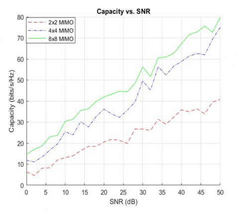
Figure 4 provides three different transmitter and receiver of 2×2, 4×4, and 8×8 MIMO. The capacity of each configuration is measured and plotted against varying SNR values. As the SNR increases, the capacity of all MIMO configurations also increases. This is expected since higher SNR implies better signal quality and less interference from noise. The 2×2 MIMO configuration has the lowest capacity among the three configurations throughout the SNR range, resulting in a less spatial multiplexing gain. The 4×4 MIMO configuration exhibits higher capacity than the 2×2 configuration. It can exploit spatial diversity and multiplexing gain, leading to improved capacity. The 8×8 MIMO demonstrates the highest capacity among the three configurations. Increasing the number of antennas improves capacity, but there are diminishing returns with each additional antenna led depends on cost, size, power consumption, and implementation complexity.
Figure 4. Capacity vs. SNR of many different MIMO
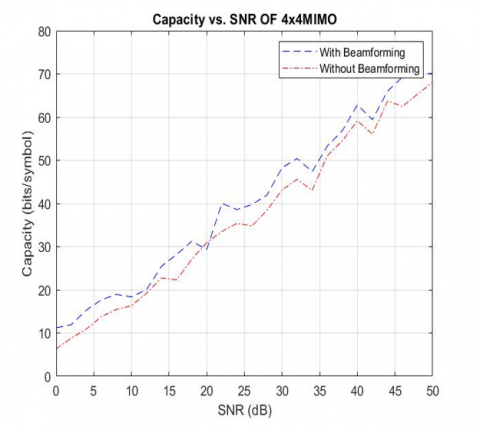
Figure 5 illustrates the communication capacity versus SNR for a 4×4 MIMO system. Two scenarios are compared: one with beamforming (depicted by the blue dashed line) and the other without beamforming (depicted by the red dash-dot line). As the SNR increases, the capacity improves in both cases, but the capacity is notably higher with beamforming. This visual representation highlights the effectiveness of beamforming in enhancing the communication system's capacity under varying SNR conditions. this indicates that beamforming effectively enhances capacity of direct D2D connection systems.
Figure 5. Capacity vs. SNR with/without beamforming
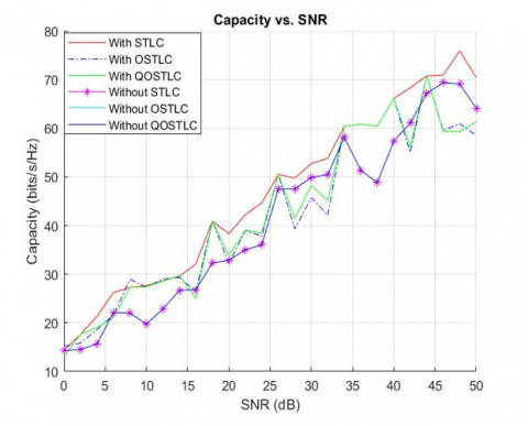
In Figure 6, with STLC, OSTLC, and QOSTLC, the capacity increases with increasing SNR. At higher SNR values, the capacities of all three beamforming techniques tend to saturate. Without STLC, OSTLC, and QOSTLC: The capacity without any beamforming also increases with increasing SNR, but the capacity is lower than those with beamforming techniques. QOSTLC yields the highest capacity, followed by OSTLC and STLC. The choice of beamforming technique can substantially impact the achievable capacity of a wireless communication system. It's worth noting that the capacity calculations assume ideal CSI at the transmitter (CSIT) and perfect channel estimation at the receiver. Additionally, the simulations assume a specific configuration with 4 transmitters and 4 receivers. The results may vary for different system configurations and channel conditions.
Figure 6. Capacity vs. SNR using STLC, OSTLC, and QOSTLC
In Figure 7, the channel capacity experiences an augmentation with rising SNR; however, this escalation occurs at a comparatively gradual pace compared to other methodologies. This phenomenon can be attributed to the utilization of a limited number of MIMO configurations. Capacity with 4×4 STLC increases with SNR and generally outperforms the 2×2 STLC. Capacity with 2×2 OSTLC increases with SNR and generally performs better than the 2×2 STLC. Capacity with 4×4 OSTLC increases with SNR and exhibits better performance than 2×2 and 4×4 STLC. Capacity with a 2×2 QOSTLC curve was added in the code, and it exhibits similar performance to the 2×2 OSTLC Capacity with 4×4 QOSTLC increases with SNR and shows improvement over the 4×4 OSTLC. The results indicate that increasing SNR for all beamforming techniques improves the system's capacity. The curves show that higher-dimensional codes, such as 4×4 OSTLC and QOSTLC, achieve higher capacity than lower-dimensional codes. Additionally, orthogonal codes generally outperform traditional codes, demonstrating the effectiveness of exploiting orthogonality in MIMO systems.
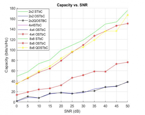
Figure 7. Capacity vs. SNR at use STLC, OSTLC, and QOSTLC of 2×2, 4×4, and 8×8 MIMO
Figure 8. Capacity vs. SNR at use of STBC, OSTBC, and QOSTBC with/without 2×2 and 4×4MIMO
Also, in Figure 8, different transmitting and receiving system, where it uses 2×2, 4×4, and 8×8 MIMO. Despite increased capacity with increasing SNR, there will be clear differences between the amount of capacity for the different model in the number of transmitters and receivers. Through our simulation of the above techniques, we have gained valuable insights into the benefits and challenges of this approach. First, we noticed that STLC-STBC encoding in a dual-hop FSO system greatly enhanced the overall performance. Implementing STLC and STBC technologies has effectively reduced fading and improved communication link reliability. This has increased the system's robustness against channel failures and through the use of orthogonal STLC-STBC also quasi-orthogonal STLC-STBC.
FSO communication is very important in 5G especially on the D2D link, minimal processing in ORD to reduce power consumption/delay is necessary when dual-hop. STLC - STBC with MIMO, improve the diversity of transmutation data in both hops, that lads decreased power consumption and delay processing. The utilize of OSTLC-OSTBC and QOSTLC-QOSTBC achieves the main purpose of this paper by balance between performance processing and reducing power consumption in the ORD. Radiation formation in the ORD also plays a role in achieving the largest amount of SNR. MATLAB simulations yielded satisfactory results. Beamforming improves system capacity, which compensates for optical signal losses, and OSTLC-OSTBC effectively achieves communication reliability, achieves minimum processing in RD, and increases system capacity. key proposals in our future work, include making communication full duplex, increasing the number of LEDs and PDs in each hop to enhance reliability, and introducing an additional RD for connectivity in case of LOS or main RD communication interruption. These actions aim to create a more robust and efficient FSO system. and further research is needed for dual-hop FSO communication techniques to meet modern communication requirements.
[1] Singh, H., Mittal, N., Miglani, R., Singh, H., Gaba, G.S., Hedabou, M. (2021). Design and analysis of high-speed free space optical (FSO) communication system for supporting fifth generation (5G) data services in diverse geographical locations of India. IEEE Photonics Journal, 13(5): 1-12. https://doi.org/10.1109/JPHOT.2021.3113650
[2] Al-Dujaili, M., Al-dulaimi, M. (2023). Fifth-generation telecommunications technologies: Features, architecture, challenges and solutions. Wireless Personal Communications, 128: 447-469. https://doi.org/10.1007/s11277-022-09962-x
[3] Sachan, A., Sarma, S.S., Hazra, R., Talukdar, F.A. (2022). Device-to-device communication in an uplink channel for a 5G mm-Wave cellular network. Preprint Research Square. https://doi.org/10.21203/rs.3.rs-1780213/v1
[4] Yaseen, M.A., Abass, A., Abdulsatar, S. (2021). Improving of wavelength division multiplexing based on free space optical communication via power comparative system. Wireless Personal Communications, 119: 1-11. https://doi.org/10.1007/s11277-021-08216-6
[5] Weng, H., Wang, W., Chen, Z., Zhu, B., Li, F. (2024). A review of indoor optical wireless communication. Photonics, 11(8): 722. https://doi.org/10.3390/photonics11080722
[6] Aboelala, O., Lee, I.E., Chung, G.C. (2022). A survey of hybrid free space optics (FSO) communication networks to achieve 5G connectivity for backhauling. Entropy, 24(11): 1573. https://doi.org/10.3390/e24111573
[7] Atiyah, M.A., Abdulameer, L.F., Narkhedel, G. (2023). PDF comparison based on various FSO channel models under different atmospheric turbulence. Al-Khwarizmi Engineering Journal, 19(4): 78-89. https://doi.org/10.22153/kej.2023.09.004
[8] Hario, F., Maulana, E., Pramono, S.H., Sari, S.N., Al Junaedi, A.M. (2019). Design of OFDM-FSO communication system on high data rate for tropical climate region. In 2019 International Conference on Advanced Technologies for Communications (ATC), Hanoi, Vietnam, pp. 74-78. https://doi.org/10.1109/ATC.2019.8924543
[9] Khattabi, Y.M., Matalgah, M.M. (2018). Alamouti-OSTBC wireless cooperative networks with mobile nodes and imperfect CSI estimation. IEEE Transactions on Vehicular Technology, 67(4): 3447-3456. https://doi.org/10.1109/TVT.2017.2786471
[10] Amodu, O.A., Othman, M., Noordin, N.K., Ahmad, I. (2021). Transmission capacity analysis of relay-assisted D2D cellular networks with interference cancellation. Ad Hoc Networks, 117: 102400. https://doi.org/10.1016/j.adhoc.2020.102400
[11] Zhu, Y., Wang, G. (2018). Research on retro-reflecting modulation in space optical communication system. IOP Conference Series: Earth and Environmental Science, 108(3): 032060. https://doi.org/10.1088/1755-1315/108/3/032060
[12] Zhong, B., Zhang, J., Zeng, Q., Dai, X. (2016). Coverage probability analysis for full-duplex relay aided device-to-device communications networks. China Communications, 13: 60-67. https://doi.org/10.1109/CC.2016.7781718
[13] Plank, T., Leitgeb, E., Pezzei, P., Ghassemlooy, Z. (2012). Wavelength-selection for high data rate Free Space Optics (FSO) in next generation wireless communications. In Proceedings of the 2012 17th European Conference on Networks and Optical Communications, Vilanova i la Geltru, Spain, pp. 1-5. https://doi.org/10.1109/NOC.2012.6249909
[14] Bagal, S., Hayagreev, V., Nazare, S., Raikar, T., Hegde, P. (2021). Energy efficient beamforming for 5G. In Proceedings of the 2021 International Conference on Recent Trends on Electronics, Information, Communication & Technology (RTEICT), Bangalore, India, pp. 928-933. https://doi.org/10.1109/RTEICT52294.2021.9573748
[15] Abdulkafi, A.A., Hardan, S.M., Bayat, O., Ucan, O.N. (2019). Multilayered optical OFDM for high spectral efficiency in visible light communication system. Photonic Network Communications, 38(3): 299-313. https://doi.org/10.1007/s11107-019-00863-x
[16] Ali, E., Ismail, M., Nordin, R., Abdulah, N.F. (2017). Beamforming techniques for massive MIMO systems in 5G: Overview, classification, and trends for future research. Frontiers of Information Technology & Electronic Engineering, 18: 753-772. https://doi.org/10.1631/FITEE.1601817
[17] Tarokh, V., Seshadri, N., Calderbank, A.R. (1998). Space-time codes for high data rate wireless communication: Performance criterion and code construction. IEEE Transactions on Information Theory, 44(2): 744-765. https://doi.org/10.1109/18.661517
[18] Sandhu, S., Heath, R., Paulraj, A. (2001). Space - time block codes versus space - time trellis codes. In Proceedings of the IEEE International Conference on Communications (ICC) (Cat. No.01CH37240), Helsinki, Finland, pp. 1132-1136. https://doi.org/10.1109/ICC.2001.936837
[19] Hacioglu, G. (2015). Space - time - frequency diversity for OFDM - based indoor power line communication. Radioengineering, 24(4): 948-955. https://doi.org/10.13164/re.2015.0948
[20] Naser, S., Bariah, L., Muhaidat, S., Al-Qutayri, M., Uysal, M., Sofotasios, P.C. (2021). Space - time block coded spatial modulation for indoor visible light communications. IEEE Photonics Journal, 13(1): 1-14. http://doi.org/10.1109/JPHOT.2021.3126873
[21] Tubail, M.A., Abu-Hudrouss, A.M., El Astal, M.T.O. (2020). Super-orthogonal double space–time trellis code. Physical Communication, 41: 101110. http://doi.org/10.1016/j.phycom.2020.101110
[22] Li, L., Fang, Z., Zhu, Y., Wang, Z. (2008). Generalized differential transmission for STBC systems. In Proceedings of the 2008 IEEE Global Telecommunications Conference (IEEE GLOBECOM 2008), New Orleans, LA, USA, pp. 1-5. https://doi.org/10.1109/GLOCOM.2008.ECP.836
[23] Celebi, M.E., Sahin, S., Aygolu, U. (2007). Full rate full diversity space-time block code selection for more than two transmit antennas. IEEE Transactions on Wireless Communications, 6(1): 16-19. http://doi.org/10.1109/TWC.2006.05005
[24] Granados, O., Andrian, J. (2011). Space-time block coding with symbol-wise decoding for polynomial phase modulated signals. In Proceedings of the 2011 Wireless Telecommunications Symposium (WTS), New York, NY, USA, pp. 1-7. https://doi.org/10.1109/WTS.2011.5960851
[25] Yang, L., Guo, W., Ansari, I.S. (2020). Mixed dual-hop FSO-RF communication systems through reconfigurable intelligent surface. IEEE Communications Letters. http://doi.org/10.1109/LCOMM.2020.2986002
[26] Urosevic, U. (2023). Low-complexity dual-hop D2D design. IEEE Transactions on Consumer Electronics, 69(3): 548-555. https://doi.org/10.1109/TCE.2023.3278628
[27] Youn, J., Yeom, J.S., Joung, J., Jung, B.C. (2023). Cooperative space-time line code for relay-assisted Internet of Things. ICT Express, 9(2): 253-257. http://doi.org/10.1016/j.icte.2022.07.004
[28] Khalid, A., Suksompong, P. (2024). Application of maximum rank distance codes in designing of STBC-OFDM system for next-generation wireless communications. Digital Communications and Networks, 10(4): 1048-1056. https://doi.org/10.1016/j.dcan.2022.12.022
[29] Alathwary, W.A., Altubaishi, E.S. (2023). Performance analysis of dual-hop DF multi-relay FSO system with adaptive modulation. Applied Sciences, 13(19): 11035. https://doi.org/10.3390/app131911035
[30] Ansari, I.S., Yilmaz, F., Alouini, M.S. (2015). Performance analysis of FSO links over unified gamma-gamma turbulence channels. In 2015 IEEE 81st Vehicular Technology Conference (VTC Spring), Glasgow, UK, pp. 1-5. http://doi.org/10.1109/VTCSpring.2015.7145999