Python Simulations for Engineering Education: Resultant and Equilibrium in Coplanar Non-Concurrent Forces

Learning forces and their effects on physical systems is a fundamental thing in the field of engineering and physics. Coplanar and non-concurrent forces (which are the specific class of forces) are the focus of this article. These forces share the property of acting in the same plane but do not intersect at a common point [2]. Understanding the calculation principles behind the resultant forces and their equilibrium is central in numerous engineering applications, such as structural analysis and mechanical design. In the context of structural engineering and the analysis of beams, the principles related to coplanar and non-concurrent forces take on particular significance. Beams, whether cantilevered or simply supported, are critical components of various structures, and understanding how forces act on them is necessary for confirming structural stability and performance [27]. This section will elaborate on the theoretical concepts of coplanar non-concurrent forces, providing a deeper insight into the mathematical principles underpinning their analysis.

The concept of the resultant force is important to understand the net effect of multiple forces acting on a system. For a system the resultant force is the single force that produces the same effect as the original forces combined when applied at the appropriate point [28]. To determine the resultant force, vector addition is employed, a mathematical method that considers both the magnitude and direction of forces.

In this article (in Python formulation), forces are treated as vectors, which are mathematical entities that have both magnitude and direction. An arrow usually represents a vector and can be expressed in the form: F=[HV], where, H represents the horizontal component and V represents the vertical component of the forece F.

For a system of non-concurrent forces, each force is represented as a vector, and all vectors are considered in the same plane, simplifying the analysis. The vector addition allows us to find the resultant force vector, which, when clubbed with the following steps, will lead to support reactions and moments [1, 3, 6]:

• Resolve external forces into components, i.e., each force in the system is resolved into its horizontal and vertical components. This step involves breaking down each force vector into its constituent parts based on the system's geometry.
• Sum up all the horizontal components and equate them to zero for the equilibrium condition.
• Sum up all the vertical components and equate them to zero for the equilibrium condition.
• If the end is fixed, then the moment will be the sum of all the moments. Whereas, if it is hinge, the sum of the moments will be equal to zero.

2.1 Common type of loadings

In structural engineering, various types of loads come upon, each of which exerts different forces on a structure. Understanding and analysing these loads is necessary for designing safe and efficient structures. Here are some commonly seen loadings [4, 6, 27]:

• Concentrated loads: Concentrated loads are the point loads that act at specific location/point on a structure. These loads are usually represented by forces applied at a single point or distributed over a small area. Examples of concentrated loads include the weight of a person standing on a floor or the force applied by a vehicle's tire on a bridge.
• Uniformly distributed loads (UDL): UDL, often called as uniform loads, are the one which are distributed evenly along a specific span of a structure. These loads are usually represented by a force per unit length (e.g., N/m). Common examples of UDLs include the self-weight of beams, uniform snow loads on a roof, or wind pressures acting along the building height.
• Uniformly varying loads (UVL): Uniformly varying loads are distributed loads that change linearly along the length of a structural element. A triangular distribution of force often represents these types of loads. An example of a uniformly varying load is the hydrostatic pressure on the side of a dam, which increases with depth.
• External moments: External moments, also known as applied moments, are twisting forces applied to a structure. These moments can occur at specific points or along the length of a beam or other structural element. For instance, a door on hinges applies an external moment to its frame.

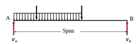
Figure 1 shows these loads from the point of view of a simply supported beam (the same holds for the cantilever as well). Engineers must consider the effects of these various loadings during the design and analysis of buildings, bridges, and other structures to ensure they can safely support the forces they encounter. By understanding and appropriately accounting for these loads, engineers can create safe, efficient and durable structures.

1.png

Figure 1. Different types of loads acting on a simply supported beam

2.2 Commonly used beams

• Cantilever beams: A cantilever beam is a structural element supported at one end while the other remains free. This type of beam is common in constructions like balconies and diving boards. Understanding how to calculate the resultant of coplanar non-concurrent forces is essential for assessing the stability and strength of cantilever beams. When multiple forces are applied to a cantilever beam, they may not intersect at a single point. Each force must be broken down into horizontal and vertical components to find the resultant support forces. The summation of these components provides the resultant horizontal and vertical reaction forces. The net moment of all the vertical force at the support has to be evaluated for the support moment. In practical terms, calculating the resultant force is essential to assess a cantilever beam's bending moment, shear forces, and deflections. This analysis ensures that the beam can withstand the loads applied to it, safeguarding against structural failure and ensuring the safety of occupants. In this beam, there are three reaction components at the fixed end, and at the free end, no reaction is there. A typical cantilever beam is shown in Figure 2.
• Simply supported beams: A simply supported beam is another common structural element. It is supported at both ends (both ends hinged or one end hinged and the other having a roller), allowing it to rest on external supports, such as walls or columns. This type of beam can be found in floor systems, bridges, and roof trusses. Analysing the resultant of coplanar non-concurrent forces is essential for designing and evaluating the performance of simply supported beams. Similar to cantilever beams, multiple forces can act on simply supported beams. The process of finding the support reactions remains the same, but as the supports are either hinged or have rollers, the moment will be zero there. Assessing the beam's reaction forces at its supports is vital for structural design and ensuring equilibrium. Engineers must determine whether the beam is under tension or compression and evaluate its deformation under the applied loads. A typical simply supported beam having both ends hinged, and one hinged and the other on rollers is shown in Figures 3(a) and (b), respectively.

• Overhanging beams: This type of beam is projected beyond the supports. The overhang can be on either side of the supports, as shown in Figure 4.

In this article, the statically determinate beams are considered as these beams are the ones in which all reaction components can be obtained with the help of above-mentioned equilibrium conditions.

2.png

Figure 2. A typical cantilever beam

31.png

(a) Simply supported beam

32.png

(b) One end fixed and the other on roller

Figure 3. Typical simply supported beams

33.png

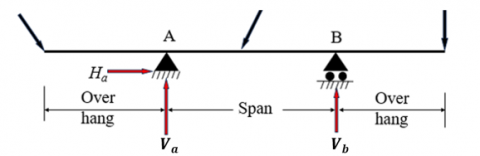
(a) Single overhang

34.png

(b) Double overhang

Figure 4. Typical schematic of overhanging beams

2.3 Reaction calculations

Cantilever beams

1. Point loads: For the point loading shown in Figure 5, the reactions and moments at the fixed end ($H_a, V_a$, and $M_a$) are evaluated as:

5.png

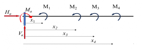
Figure 5. Point loads acting on the cantilever

$V_a=\sum_{i=1}^{i=n} F_i \sin \left(\theta_i\right)$          (1)

$H_a=\sum_{i=1}^{i=n} F_i \cos \left(\theta_i\right)$             (2)

$M_a=\sum_{i=1}^{i=n}\left(F_i \sin \left(\theta_i\right) \times x_i\right)$          (3)

2. UDL: For UDL’s shown in Figure 6, the reactions and moments at the fixed end are evaluated as:

6.png

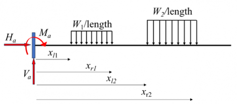
Figure 6. UDL acting on cantilever

$V_a=\sum_{i=1}^{i=n} W_i\left(x_{r i}-x_{l i}\right)$           (4)

$H_a=0$            (5)

$M_a=\sum_{i=1}^{i=n} W_i\left(x_{r i}-x_{l i}\right)\left(x_{r i}+x_{l i}\right) / 2$            (6)

3. UVL: For UVL, as shown in Figure 7, the reactions are evaluated as shown in Eqs. (7) and (8), but the lever arm for the moment at the fixed end are evaluated considering two cases viz. case-I and case-II.

7.png

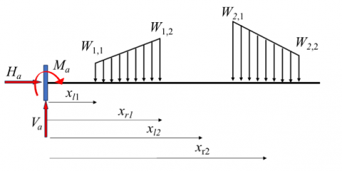
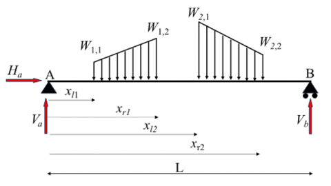
Figure 7. UVL acting on the cantilever

$V_a=\sum_{i=1}^{i=n}\left(\frac{1}{2}\right)\left(W_{i, 1}+W_{i, 2}\right)\left(x_{r i}-x_{l i}\right)$        (7)

$H_a=0$            (8)

$M_a=\sum_{i=1}^{i=n}\left(\frac{1}{2}\right)\left(W_{i, 1}+W_{i, 2}\right)\left(x_{r i}-x_{l i}\right) \times \ell_i$           (9)

Case-I: The left end load of UVL is lower than the right load

$\ell_i=\left(x_{l i}+\left(x_{r i}-x_{l i}\right)\left(1-\frac{W_{i, 2}+2 W_{i, 1}}{W_{i, 1}+W_{i, 2}} \times \frac{1}{3}\right)\right)$        (10)

Case-II: The right end load of UVL is lower than left load

$\ell_i=\left(x_{l i}+\frac{\left(x_{r i}-x_{l i}\right)}{3}\left(\frac{W_{i, 1}+2 W_{i, 2}}{W_{i, 1}+W_{i, 2}}\right)\right)$           (11)

8.png

Figure 8. External moments acting on cantilever

4. External moments: For external moments shown in Figure 8, the reactions at the support are evaluated as:

$V_a=0$       (12)

$H_a=0$       (13)

$M_a=\sum_{i=1}^{i=n} M_i$         (14)

Simply supported beam

In case of simply supported beam as the moment at the reactions is zeros so in the calculations they are not been taken into account.

1. Point loads: For the point loading shown in Figure 9 the reactions at the supports ($H_a, V_a, V_b$, and $M_a$) are evaluated as:

$V_b=\frac{1}{L} \sum_{i=1}^{i=n}\left(F_i \sin \left(\theta_i\right) \times x_i\right)$            (15)

$H_a=\sum_{i=1}^{i=n} F_i \cos \left(\theta_i\right)$        (16)

$V_a=\sum_{i=1}^{i=n} F_i \sin \left(\theta_i\right)-V_b$          (17)

9.png

Figure 9. Point loads acting on simply supported beam

2. UVL: For UVL’s shown in Figure 10, the reactions at the supports are evaluated as:

10.png

Figure 10. UVL acting on simply supported beam

$V_b=\left(\frac{1}{2 L}\right) \sum_{i=1}^{i=n}\left(W_{i, 1}+W_{i, 2}\right)\left(x_{r i}-x_{l i}\right) \times \ell_i$        (18)

$H_a=0$           (19)

$V_a=\left(\frac{1}{2}\right) \sum^{i=n}\left(W_{i, 1}+W_{i, 2}\right)\left(x_{r i}-x_{l i}\right)-V_b$          (20)

For $\ell_i$, Eqs. (10) and (11) will be used.

3. UDL: For UDL’s shown in Figure 11, the reactions at the supports are evaluated as:

11.png

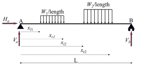
Figure 11. UDL acting on simply supported beam

$V_b=\left(\frac{1}{2 L}\right) \sum_{i=1}^{i=n} W_i\left(x_{r i}-x_{l i}\right)\left(x_{r i}+x_{l i}\right)$         (21)

$H_a=0$        (22)

$V_a=\sum_{i=1}^{i=n} W_i\left(x_{r i}-x_{l i}\right)-V_b$           (23)

4. External moments: For external moments shown in Figure 12, the reactions at the support are evaluated as:

12.png

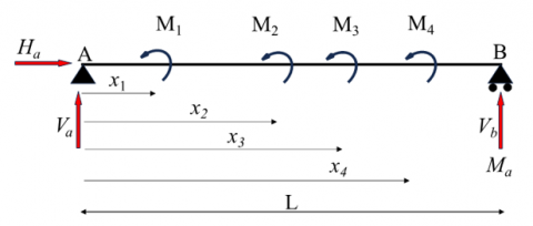
Figure 12. External moments acting on simply supported beam

$V_b=\left(\frac{1}{L}\right) \sum_{i=1}^{i=n} M_i$        (24)

$H_a=0$             (25)

$V_a=-V_b$          (26)

Point to be noted in all the above calculations is that downward loading is considered as positive. All the angles are measured counter-clock wise. For cantilever the x coordinate starts at fixed end whereas, for simply supported beam it will start from left support.

In this section all the Python functions developed above are tested against different types of loadings on cantilever and simply supported beams.

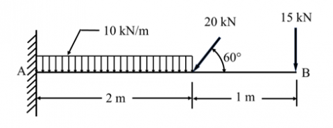
Example 1: For the cantilever beam shown below in Figure 13, evaluate the fixed end reactions:

13.png

Figure 13. Cantilever beam with UDL and point load

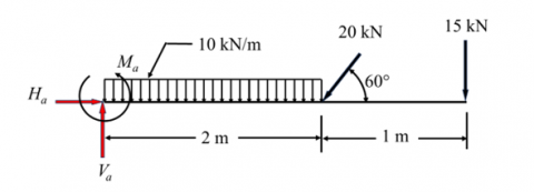
Solution: Figure 14 represents the forces, reactions and moments acting on the beam shown in Figure 13.

14.png

Figure 14. FBD

This problem has two types of loads viz. point load and udl. The functions used are: canti_pl (w,θ,x) and canti_udl (w,θ,x). The program to call the functions and its output is as follows:

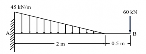
Example 2: For the cantilever beam shown below in Figure 15, evaluate the fixed end reactions:

15.png

Figure 15. Cantiler beam with UVL and point load

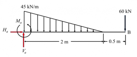
Solution: Figure 16 represents the forces, reactions and moments acting on the beam shown in Figure 15.

16.png

Figure 16. FBD

This problem has two types of loads viz. point load and uvl. The functions used are: canti_pl (w,θ,x) and canti_uvl (w,θ,x). The program to call the functions and its output is as follows:

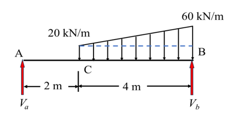
Example 3: For the simply supported beam shown below in Figure 17, evaluate the reactions at the end:

17.png

Figure 17. Cantilever beam with UVL

Solution: Figure 18 represents the forces and reactions acting on the beam shown in Figure 17.

18.png

Figure 18. FBD

This problem has only uvl. The functions used is: ssb_uvl (w,x,L). The program to call the functions and its output is as follows:

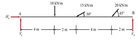
Example 4: For the simply supported beam and its FBD shown below in Figure 19, evaluate the reactions at the end:

19.png

Figure 19. Simply supported beam with point loads

Solution: Figure 20 represents the forces and reactions acting on the beam shown in Figure 19.

20.png

Figure 20. FBD

This problem has only point loads. The functions used is: ssb_pl(w,θ,x,L). The program to call the functions and its output is as follows:

Example 5: For the simply supported beam shown below in Figure 21, evaluate the reactions at the end:

21.png

Figure 21. Simply supported beam with UVL and point loads

Solution: This problem has point loads and udl. The functions used are: ssb_pl (w,θ,x,L) and ssb_udl (w,x,L). The program to call the functions and its output is as follows:

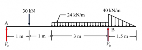
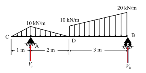
Example 6: For the simply supported beam shown below in Figure 22, evaluate the reactions at the end:

22.png

Figure 22. FBD of an over hanging beam

Solution: This problem has point load, uvl, and udl. The functions used are: ssb_pl(w,θ,x,L) , ssb_udl(w,x,L), and ssb_uvl(w,x,L). The program to call the functions and its output is as follows:

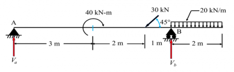
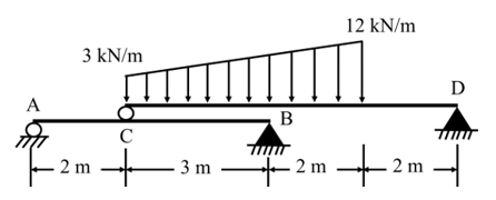
Example 7: For the overhanging beam shown below in Figure 23, evaluate the reactions at the end:

23.png

Figure 23. Overhanging beam with moment, point load, and UDL

Solution: This problem has point load, external moment, and udl. The functions used are: ssb_pl(w,θ,x,L), ssb_udl(w,x,L), and ssb_mom(w,x,L). The program to call the functions and its output is as follows:

Example 8: For the simply supported beam shown below in Figure 24, evaluate the reactions at the end:

24.png

Figure 24. Overhanging beam with UVL

Solution: This problem has two uvl’s. The function used is: ssb_uvl(w,x,L). The program to call the functions and its output is as follows:

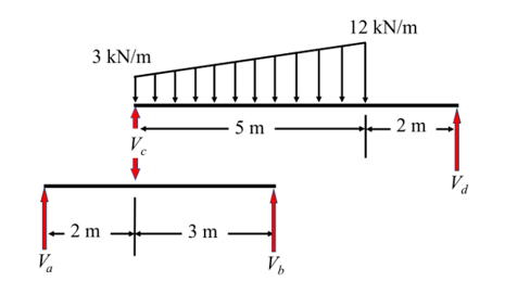
Example 9: For the simply supported beam shown below in Figure 25, evaluate the reactions at the end:

25.png

Figure 25. A complex beam

Solution: Free body diagrams of beams AB and CD are shown below in Figure 26.

26.png

Figure 26. FBD

This problem has one uvl but if looked closely, then the problem can be divided into two. First, the top beam has to be solved with uvl, which will result in a reaction at roller and D. Then the reaction at C will act as a point load for the bottom beam, which now can be solved for the reactions at A and B. The function used is: ssb_udl(w,x,L), and ssb_pl(w,x,L). The program to call the functions and its output is as follows:

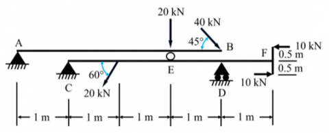
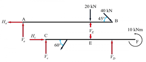
Example 10: For the simply supported beam shown below in Figure 27, evaluate the reactions at the end:

27.png

Figure 27. Arrangements of overhanging beams

28.png

Figure 28. FBD

Solution: The free body diagram of beams shown in Figure 26 is shown in Figure 28.

This problem also has two beams to solve. First, the top beam has to be solved with two-point loads, resulting in reaction at E and A. Then, the reaction at E will act as a point load for the bottom beam, which now can be solved for the reactions at C and D. Also, there is one moment acting at F of magnitude 10 N-m. The function used is: ssb_pl (w,θ,x,L), and ssb_mom (w,x,L). The program to call the functions and its output is as follows:

While this study largely focuses on theoretical examples, the developed Python functions can be readily applied to a variety of real-world engineering situations as well. For instance, they can be used in structural analysis for designing safe and stable buildings, bridges, and mechanical systems subjected to multiple forces and moments. These functions can also serve as an educational tool to help the students understand the principles of statics and equilibrium in a more collaborative and practical way.