Ayoub El Yousfi*![]() | Yaser Alawi
| Yaser Alawi![]()
© 2025 The authors. This article is published by IIETA and is licensed under the CC BY 4.0 license (http://creativecommons.org/licenses/by/4.0/).
OPEN ACCESS
Unmanned aerial vehicles (UAVs), also known as drones, are increasingly used for various purposes such as photography, surveillance, mapping, inspection, and agriculture. This research specifically focuses on agricultural drones, which have the potential to address challenges encountered by farmers, ultimately positively affecting crop yields. Their ability to apply pesticides accurately and autonomously, without direct human involvement, is crucial for modern farming practices. This study aims to design and simulate a quadcopter specifically tailored for pesticide spraying. The design process involves careful selection of components and simulation using both SolidWorks and MATLAB Simulink. In SolidWorks, design the frame and components, while MATLAB Simulink is used to simulate trajectory tracking using PID controllers. The key finding is the integration of a multispectral camera to capture images and analyze data using Pix4Dfields and Agremo software. This analysis helps pinpoint specific areas requiring treatment, thereby minimizing pesticide and water usage while maximizing profitability. By targeting exact locations in the field based on data analysis, this approach improves efficiency. The research focuses on evaluating the quadcopter's performance and trajectory accuracy, offering valuable insights into its potential agricultural impact, and assisting farmers in enhancing their profits through improved spraying techniques and resource management.
quadcopter, unmanned aerial vehicles, PID controller, agricultural, trajectory tracking
UAVs are aircraft that operate without a human pilot, using inertial sensors and navigation technology to fly either remotely or autonomously [1]. UAVs are categorized based on the number of rotors in their platforms [2], with the main types being fixed-wing [3], helicopter, and multi-copter [4]. These UAVs have revolutionized various sectors, including agriculture, where they hold significant promise for improving farming practices [5].
Traditional spraying systems often lack precision, leading to overuse of pesticides and causing health risks to humans, harm to beneficial organisms, and soil degradation [6]. The World Health Organization (WHO) predicts that up to one million people could be adversely affected by pesticide exposure in crop fields [7]. UAVs offer better, targeted spraying solutions [8]. Multi-copter UAVs, especially quadcopters, balance coverage and maneuverability, making them perfect for precision agriculture [9]. With multispectral cameras and software like Pix4Dfields and Agremo, they improve pesticide accuracy, reduce chemical use, and increase crop yield. These benefits highlight the importance of UAVs in modern agriculture to address the problems of traditional methods.
This research aims to design and simulate a quadcopter specifically tailored for agricultural pesticide spraying. By utilizing advanced imaging and data analysis tools, such as multispectral cameras, Pix4Dfields, and Agremo software, the proposed solution seeks to optimize pesticide application. This approach addresses the inefficiencies and environmental concerns of current technologies, providing a more precise and efficient method for modern farming practices.
Control systems such as the Linear Quadratic Gaussian (LQG), Linear Quadratic Regulator (LQR), and the Proportional-Integral-Derivative (PID) controller [10, 11] play a pivotal role in managing both the position and orientation of quadcopters. Central to these systems is the Plant block, which encompasses a detailed mathematical model of the entire system, including motor mixing [12].
Quadrotors have attracted considerable interest from the research community due to their adaptability and potential applications in various sectors. These drones are increasingly used in fields such as surveillance, mapping, and agriculture, where they perform tasks like pesticide spraying and crop monitoring [13]. This study specifically investigates a quadcopter designed for agricultural spraying, focusing on the selection of components and testing the durability of the frame under various forces. Additionally, simulation experiments will be conducted in MATLAB to control the drone’s flight trajectory using PID controllers. Through this research, we aim to enhance our understanding of how quadcopters can be effectively utilized in agriculture, thereby contributing to technological advancements in this area.
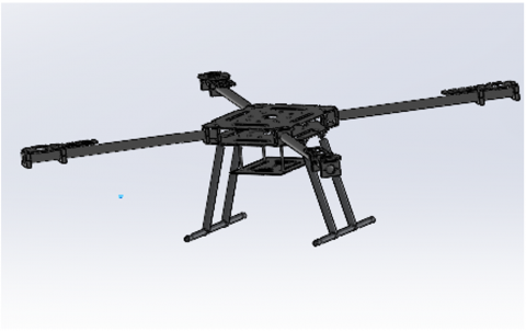
Drones have transformed transportation, photography, surveillance, and agriculture. This study uses a carbon fiber frame like the Tarot Ironman with diagonal 685, ideal for lightweight missions. Figure 1 highlights the quadcopter design, emphasizing efficiency. All components were designed in SolidWorks. Advances in sensor technology have enabled the creation of smaller UAVs like this quadcopter [14].
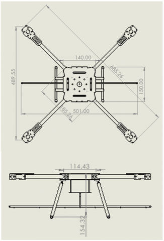
Figure 2 shows that the frame of the drone has 685 ± 1 mm diagonal distance between motors in the drone frame significantly impacts its size, stability, agility, and payload capacity, potentially enabling larger payloads or specialized equipment.
The selection of drone components is crucial for estimating our payload and ensuring mission success. The motor plays a vital role in this type of mission. Drones use propellers, motors, and ESCs for various tasks. The optimal setup depends on the drone's intended functions. Estimating the weight and dimensions of the payload is the first step in determining the ideal setup for a drone.
Figure 1. Drone frame designed
Figure 2. Drone dimensions
Figure 3. Payload dimensions
The payload is designed to hold the multispectral camera and the spraying tube. It is engineered for easy implementation. Figure 3 shows the dimensions of the holder for the tube and camera, which are made from carbon fiber.
2.1 Payload estimation
To ensure the success of the payload mission, it is crucial to accurately calculate the drone's total weight, including the water, to make informed decisions about its capabilities. The payload consists of components like the tube and sprayer for pesticide application. Specifically, for a 20-meter tube with a 12-millimeter inner diameter, calculations are required to determine the payload's weight by first calculating the cross-sectional area of the tube.
$A=\pi \times\left(R_o^2-R_i^2\right)$ (1)
$R_o=\frac{Outer diameter}{2}=\frac{15.4}{2}=7.7 \mathrm{~mm}$
$R_i=\frac{inner diameter}{2}=\frac{12}{2}=6 \mathrm{~mm}$
where, $R_0$ is the outer radius and $R_i$ is the inner radius.
Now we can find the cross-sectional area $A$.
$A=\pi \times\left(7.7^2-6^2\right)=73.161 \mathrm{~mm}^2$
The volume of water passing through the tube:
Volume $=A \times$ Lengh (2)
Volume = 73.161×20000 mm = 1.456.220 mm3
The estimated weight of water, assuming a density of approximately 1 kg/L, would be approximately 1.463 kg for a length of 20 meters passing through the tube.
The total weight (WT) of the tube is determined based on a specified tube length of 20 meters.
WT = Weight of the tube + Weight of water =3.263 kg
This calculation assumes the tube is filled with water, and the weight is an approximation based on the volume of water considering its density. The total estimation of the drone after defining the payload estimation will be.
For the quadcopter designed for mission spraying and carrying out large payload capacity, a motor with a high throttle is needed to carry the weight of the drone. Determination of the suitable motors and propellers for your drone, needs to calculate the thrust generated at 100% RPM based on the total weight carried. This calculation is crucial for selecting components that can handle your specific payload requirements and the demands of your mission as shown in Table 1.
Thrust $=\frac{\text { The total weigh } \times 2}{\text { The numebr of rotors }}$ (3)
To achieve the desired weight parameters, it's crucial to calculate the thrust required for each motor and propeller combination at 100% RPM, ensuring the propulsion system can effectively support and lift the drone, for our drone the weight should left per motor after dividing the total thrust generated is 14,465 grams, indicating that each motor needs to produce an additional 3,615.5 grams of thrust to meet the required total thrust. The motor selection will be determined based on the derived results indicating the required thrust specifications.
Table 1. Main dimensions and geometry parameters of the model
|
Components |
Mass (g) |
|
Tube + the mass of water pass through it |
3263 |
|
Frame (body of drone) |
500 |
|
4×Motors |
1000 |
|
4×Propellers 15×5 |
164 |
|
Battery |
max1600 |
|
ECS |
104 |
|
Other components (cables-screw) |
100 |
|
Pump and nozzle |
500 |
|
Total |
7231-MAX 8000 |
2.2 The motor and propeller selection
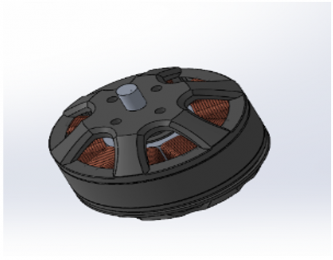
Brushless DC motors are preferred for drones due to their limited maintenance, high efficiency, and reduced noise [15]. They feature a permanent magnet rotor and electronic commutation, offering accurate control and longer flight times. With an added weight of 7231 g, doubling the initial weight to about 14462 g, the chosen T-MOTOR MN5212 (420 KV) motors as shown in Figure 4, paired with a 381 mm by 127 mm propeller, generate a theoretical lifting force of 4157 g per motor.
The drone's performance is optimized with a 15-inch diameter propeller and 5-inch pitch, paired with the T-MOTOR MN5212, which reaches over 9000 RPM. This setup meets the thrust requirements for the drone's intended use. The ECS AIR 40A ESC ensures optimal performance for this motor and propeller combination. The system also includes Pixhawk, GPS, and a 12000mAh LiPo battery (4-6s) to meet operational needs efficiently.
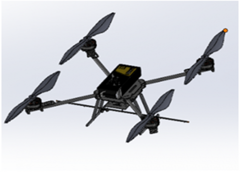
The final assembly of the spraying quadcopter drone includes motors, propeller, and ECS, along with a Flight controller that manages and controls the vehicle's flight dynamics, ensuring stability, responsiveness, and control throughout the flight as shown in Figure 5. Additionally, the inclusion of the "Blue tube" within this setup is critical, serving a specific purpose that justifies its placement within the overall system. The ECS AIR 40A ESC ensures optimal performance and stability in the drone's intended application, such as aerial platforms or drones.
Multispectral imaging is essential for precision agriculture, identifying areas needing pesticide application [16]. Using a Parrot Sequoia+ multispectral camera, a drone captures images at various wavelengths, including near-infrared, red-edge, and visible light bands, providing a detailed view of vegetation and its environment [17].
Figure 4. T-motor MN5212 420 KV
Figure 5. The final assembly of quadcopter drone
Figure 6. Parrot Sequoia +
The Parrot Sequoia + is a high-precision camera that captures multispectral imagery, enabling detailed analysis of vegetation health, stress levels, and growth patterns as shown in Figure 6. Its unique characteristics provide valuable insights into the composition and condition of vegetation.
Our research integrates the Parrot Sequoia + multispectral camera into the drone, enhancing our understanding of vegetation and ecosystem health. This technology will help advance precision agriculture, environmental monitoring, and land management.
2.3 Data analysis
Healthy plants reflect 10% green light and nearly 50% of near-infrared (NIR) wavelengths. This study uses Normalized Difference Vegetation Index (NDVI) to assess green density by measuring light at 660 nm (dark red) and 740 nm (red edge). NDVI helps detect plant diseases, with data collected by drones and analyzed using computer vision and machine learning software [18].
Pix4Dfields is an agricultural software that uses multispectral and RGB drone imagery to analyze vegetation, monitor crops, and map fields, aiding informed decision-making and improving field health.
Figure 7. Pix4Dfield for image processing and analysis
Figure 8. Argemo interface overview
Pix4Dfields is a drone-based software for agricultural mapping and analysis, ideal for crop health monitoring and yield estimation but requires time and knowledge to tailor solutions as shown in Figure 7. Agremo uses advanced algorithms and AI to process multispectral and RGB imagery, offering actionable insights and valuable statistics on crop and vegetation health as shown in Figure 8.
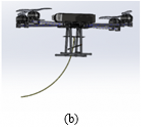
Drones are revolutionizing agriculture with advanced crop spraying but face challenges in stability and payload management. Stability is crucial for pesticide spraying, requiring powerful motors to handle heavy loads and spray tubes for even distribution. Effective design must balance payload capacity, energy efficiency, and aerodynamics to ensure precision and stability, optimizing crop yield for large-scale farming as shown in Figure 9.
A 2.5-meter support system has been added to drones for large-area crop spraying to enhance precision and stability. It holds the water tube, ensuring steadiness and uniform spray distribution. This innovation improves payload management and stability, allowing drones to operate efficiently over larger fields with reduced risk of drift or instability.
Figure 9. (a) Drone equipped with tubing for spraying operations; (b) The implementation of support system
Mathematical modeling is essential for understanding dynamic reactions, governing equations, and controller design, while also providing useful non-linear equations for understanding physical systems [19].
To simplify our mathematical modeling, we assume the drone and its propellers are rigid bodies with symmetry across all axes. We also neglect complex fluid dynamic effects, focusing on thrust, pitch, yaw, and roll control. These assumptions help approximate real-world conditions without adding excessive complexity.
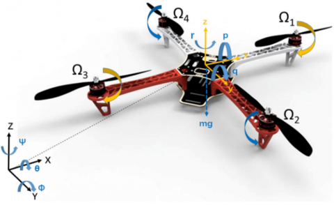
The quadrotor structure is presented in Figure 10 including the corresponding angular velocities, torques and forces created by the four rotors (numbered from 1 to 4).
Figure 10. Body axis and inertial axis system
The absolute linear position of the quadrotor is defined in the inertial frame $x, y, z$ axes with $\boldsymbol{\lambda}$. The angular position is defined in the inertial frame with three Euler angles $\eta$. Pitch angle $\theta$ determines the rotation of the quadrotor around the $y$ axis. Roll angle $\varphi$ determines the rotation around the x -axis and yaw angle $\psi$ around the $z$-axis [20].
The origine of the body frame is in the center of mass of the quadrotor. The linear velocities in the body frame are determined by $V_B$ and the angular velocities by $\omega_{\mathrm{B}}$ :
$$
V_I=\left[\begin{array}{c}
\dot{x} \\
\dot{y} \\
\dot{z}
\end{array}\right], \omega_E=\left[\begin{array}{c}
\dot{\varphi} \\
\dot{\theta} \\
\dot{\psi}
\end{array}\right], V_B=\left[\begin{array}{c}
u \\
v \\
w
\end{array}\right], \omega_B=\left[\begin{array}{l}
p \\
q \\
r
\end{array}\right], \lambda=\left[\begin{array}{c}
X \\
Y \\
Z
\end{array}\right], \eta=\left[\begin{array}{c}
\varphi \\
\theta \\
\psi
\end{array}\right]
$$
where, $V_I$ represents the linear velocities and $\omega_E$ represents the Euler angle rates in the inertial frame. $V_B$ is the linear and $\omega_{\mathrm{B}}$ is the angular velocity vector in the body frame.
The rotation matrix for rotation about Z-Axis, Y-Axis and X-Axis [21].
$\begin{gathered}R_z(\psi)=\left[\begin{array}{ccc}c \psi & s \psi & 0 \\ -s \psi & c \psi & 0 \\ 0 & 0 & 1\end{array}\right], R_y(\theta)=\left[\begin{array}{ccc}c \theta & 0 & -s \theta \\ 0 & 1 & 0 \\ s \theta & 0 & c \theta\end{array}\right], \\ R_x(\varphi)=\left[\begin{array}{ccc}1 & 0 & 0 \\ 0 & c \varphi & s \varphi \\ 0 & -s \varphi & c \varphi\end{array}\right]\end{gathered}$
The transformation from Inertial to body and body to inertial frame becomes $(R)$, not that $\mathrm{c}=\cos , \mathrm{s}=\sin$
$\begin{aligned}
& R_I^B=R(\varphi) R(\theta) R(\psi) =\left[\begin{array}{ccc}
c \theta c \psi & -c \theta s \psi & -s \theta \\
s \theta s \varphi c \psi+s \psi c \phi & s \psi s \theta s \varphi+c \psi c \varphi & s \varphi c \theta \\
s \theta c \varphi c \psi+s \psi s \phi & s \psi s \theta c \varphi-c \psi s \varphi & c \varphi c \theta
\end{array}\right]
\end{aligned}$ (4)
The transformation from body to inertial frame becomes:
$R_B^I=\left[\begin{array}{ccc}c \psi c \theta & s \theta c \psi s \varphi-s \psi c \varphi & c \theta s \psi c \varphi-s \psi s \varphi \\ s \psi c \theta & s \theta s \psi s \varphi+c \psi c \varphi & s \theta s \psi c \varphi-c \psi s \varphi \\ -s \theta & c \theta s \varphi & c \theta s \varphi\end{array}\right]$
4.1 Translation motion
$\begin{gathered}{\left[\begin{array}{c}\dot{x} \\ \dot{y} \\ \dot{z}\end{array}\right]=\left[R_B^I\right]\left[\begin{array}{c}u \\ v \\ w\end{array}\right]} =\left[\begin{array}{ccc}c \psi c \theta & s \theta c \psi s \varphi-s \psi c \varphi & c \theta s \psi c \varphi-s \psi s \varphi \\ s \psi c \theta & s \theta s \psi s \varphi+c \psi c \varphi & s \theta s \psi c \varphi-c \psi s \varphi \\ -s \theta & c \theta s \varphi & c \theta s \varphi\end{array}\right]\left[\begin{array}{c}u \\ v \\ w\end{array}\right]\end{gathered}$ (5)
The linear velocity equations in the inertial frame are:
$\begin{gathered}\dot{x}=(c \psi c \theta) u+(s \theta c \psi s \varphi-s \psi c \varphi) \\ +(c \theta s \psi c \varphi-s \psi s \varphi)\end{gathered}$ (6)
$\begin{gathered}\dot{y}=(s \psi c \theta) u+(s \theta s \psi s \varphi+c \psi c \varphi) v \\ +(s \theta s \psi c \varphi-c \psi s \varphi) w\end{gathered}$ (7)
$\dot{z}=-(s \theta) u+(c \theta s \varphi) v+(c \theta s \varphi) w$ (8)
4.2 Rotational motion
$\begin{gathered}\omega_B=T_E^B \times \omega_E \\ {\left[\begin{array}{l}p \\ q \\ r\end{array}\right]=\left[\begin{array}{ccc}1 & 0 & -\sin \theta \\ 0 & \cos \psi & \sin \psi \cos \theta \\ 0 & -\sin \psi & \cos \psi \cos \theta\end{array}\right] \times\left[\begin{array}{c}\dot{\varphi} \\ \dot{\theta} \\ \dot{\psi}\end{array}\right]}\end{gathered}$ (9)
Euler angle rates in body frame can be expressed as $(p q r)$ and inertial frame can be expressed as $\{\dot{\varphi}, \dot{\theta}, \dot{\psi}\}$. The set of angular equations of motion in the inertial frame can be written as:
$\left[\begin{array}{c}\dot{\varphi} \\ \dot{\theta} \\ \dot{\psi}\end{array}\right]=\left[\begin{array}{c}p+q(\sin \varphi \tan \theta)+r(\cos \varphi \tan \theta) \\ q(\cos \varphi-r \times \sin \varphi) \\ q(\sin \varphi / \cos \theta+r * \cos \varphi / \cos \theta\end{array}\right]$
4.3 Newton – Euler equations
The Newton-Euler equations are mathematically represented in the body frame as follows:
$m \dot{V}_B+m \omega_B \times V_B=\sum F_B$ (10)
$I \dot{\omega}_B+\omega_B \times I \omega_B=\sum M_B$ (11)
$m$: The mass of rigid body.
$I$: The inertia matrix.
$\sum F_B$: The external Forces.
$\sum M_B$: The external moments.
$\sum \mathrm{F}_{\mathrm{B}}=\left[\begin{array}{c}F_x \\ F_y \\ F_z\end{array}\right], \sum M_B=\left[\begin{array}{l}\mathrm{M}_{\mathrm{x}} \\ \mathrm{M}_{\mathrm{y}} \\ \mathrm{M}_{\mathrm{z}}\end{array}\right]$
4.4 Forces equations
The forces are described with the help of Eq. (10).
$\left[\begin{array}{c}F_x \\ F_y \\ F_z\end{array}\right]=m \times\left[\begin{array}{c}\dot{u} \\ \dot{v} \\ \dot{w}\end{array}\right]+\left[\begin{array}{c}p \\ q \\ r\end{array}\right] \times m\left[\begin{array}{c}u \\ v \\ w\end{array}\right]$
The linear motion equations can be expressed in terms of linear accelerations in the body frame by rearranging the dynamical equations, focusing on the accelerations along the x, y, and z axes and their relation to forces, resulting in Eq. (12).
$\left[\begin{array}{c}\dot{u} \\ \dot{v} \\ \dot{w}\end{array}\right]=\left[\begin{array}{c}\frac{F_x}{m}+r v-q w \\ \frac{F_y}{m}+(p w-r u) \\ \frac{F_z}{m}+(q u-p u)\end{array}\right]$ (12)
4.5 Moment equations
Simplified:
$\left[\begin{array}{l}M_x \\ M_y \\ M_z\end{array}\right]=\left[\begin{array}{c}L \\ M \\ N\end{array}\right]=\left[\begin{array}{l}I_{x x} \dot{p}+\left(I_{z z}-I_{y y}\right) q r \\ I_{y y} \dot{q}+\left(I_{x x}-I_{z z}\right) r p \\ I_{z z} \dot{r}+\left(I_{y y}-I_{x x}\right) p q\end{array}\right]$ (13)
To express the equations with a focus on angular accelerations, it is essential to isolate the angular accelerations on the left side of the equation. This approach yields the equations, as illustrated in the equations provided below:
$\dot{p}=\frac{1}{I_{x x}}\left[\left(I_{y y}-I_{z z}\right) q r+M_x\right]$ (14)
$\dot{q}=\frac{1}{I_{y y}}\left[\left(I_{z z}-I_{x x}\right) r p+M_y\right]$ (15)
$\dot{r}=\frac{1}{I_{z z}}\left[\left(I_{x x}-I_{y y}\right) q p+M_z\right]$ (16)
4.6 External forces
Various external forces impact the flight dynamics of a quadrotor. The collective effect of these forces determines the overall net force exerted on the quadrotor. Eq. (17) outlines the components that make up the total external forces acting on the quadrotor.
$\sum F_B=F_M+F_G+F_w$ (17)
where, $F_G$ is the gravitational force, and $F_M$ represents the force generated by the motors, and $F_w$ denotes the force exerted by the wind.
$F_M$ represents:
$F_M=\left[\begin{array}{c}0 \\ 0 \\ f_m\end{array}\right]$ (18)
where, the $f_m$ is the sum of generated by the four motors:
$f_m=f_{m 1}+f_{m 2}+f_{m 3}+f_{m 4}$ (19)
And $F_G, F_w$ are represented by the matrix below:
$F_G=R_I^B\left[\begin{array}{c}0 \\ 0 \\ m g\end{array}\right]$ (20)
$F_w=\left[\begin{array}{l}f_{w x} \\ f_{w y} \\ f_{w z}\end{array}\right]$ (21)
The external forces can be simplified by removing wind force and applying the rotation matrix to the gravity vector, as shown in Eq. (22).
$\left[\begin{array}{c}F_x \\ F_y \\ F_z\end{array}\right]=\left[\begin{array}{c}-m g(\sin \theta) \\ m g(\sin \varphi \cos \theta) \\ m(\cos \varphi \cos \theta)-f_m\end{array}\right]$ (22)
4.7 State equations
State-space representation is a robust method for describing dynamical systems, particularly beneficial for multiple input-multiple output (MIMO) systems. It consists of two main equations [22, 23]:
The state-space representation is composed of two primary equations.
$\dot{x}=A x+B u$ (23)
$y=C x+D u$ (24)
where, $u$: Control input vector, $x$: State victor, $y$: Output victor, $A$: System matrix, $B$: Input matrix, $C$: Output matrix, $D$: Feed forward matrix.
Typically, a quadcopter system encompasses twelve state variables and four control inputs. both the state variables and the control inputs can be described using the following representation.
$x$ vector and $u$ are the input vector can be written as:
$x=[\dot{x} \dot{y} \dot{z} \ddot{x} \ddot{y} \ddot{z} \dot{\psi} \dot{\theta} \dot{\varphi} \dot{p} \dot{q} \dot{r}]^T, U=\left[\begin{array}{c}U_1 \\ U_2 \\ U_3 \\ U_4\end{array}\right]$
4.8 Newton's equations of motion
Newton's equation of motion, originally formulated in the body frame, can be transposed to the inertial frame:
$m \dot{V}_I=T_B^I \sum F_I$ (25)
Forces include thrust $F_M$ and gravity $F_G$
$m \dot{V}_I=T_B^I\left[\begin{array}{c}0 \\ 0 \\ -\mathrm{U}_1\end{array}\right]+T_B^I T_I^B\left[\begin{array}{c}0 \\ 0 \\ m g\end{array}\right]=T_B^I\left[\begin{array}{c}0 \\ 0 \\ -\mathrm{U}_1\end{array}\right]+\left[\begin{array}{c}0 \\ 0 \\ m g\end{array}\right]$
4.9 Linear and angular velocities
The derivatives of the linear and angular velocities can be simplified:
$\dot{V}_I=\left[\begin{array}{c}\ddot{x} \\ \ddot{y} \\ \ddot{z}\end{array}\right]=\left[\begin{array}{c}\frac{-U_1}{m}(\cos \varphi \sin \theta \cos \psi+\sin \varphi \sin \psi) \\ \frac{-U_1}{m}(\cos \varphi \sin \theta \sin \psi-\sin \varphi \cos \psi) \\ g-\frac{U_1}{m}(\cos \varphi \cos \theta)\end{array}\right]$ (26)
Assuming small tilt angles close to zero:
$\omega_B=\omega_E$
Taking the derivative of both sides’ yields:
$\begin{aligned} & \dot{\omega}_{\mathrm{E}}=\dot{\omega}_{\mathrm{B}} \\ & {\left[\begin{array}{c}\ddot{\varphi} \\ \ddot{\theta} \\ \ddot{\psi}\end{array}\right]=\left[\begin{array}{c}\dot{\mathrm{p}} \\ \dot{\mathrm{q}} \\ \dot{\mathrm{r}}\end{array}\right]}\end{aligned}$
We can construct the final form of the derivative of the Euler rates vector, $\dot{\omega}_E$.
$\left[\begin{array}{c}\ddot{\varphi} \\ \ddot{\theta} \\ \ddot{\psi}\end{array}\right]=\left[\begin{array}{l}\frac{1}{I_{x x}}\left[\left(I_{x x}-I_{z z}\right) q r+M_x\right] \\ \frac{1}{I_{y y}}\left[\left(I_{z z}-I_{x x}\right) r p+M_y\right] \\ \frac{1}{I_{z z}}\left[\left(I_{x x}-I_{y y}\right) q p+M_z\right]\end{array}\right]$ (27)
The equations derived from the modelling of a quadrotor include twelve state variables:
$\begin{gathered}\dot{x}=(c \psi c \theta) u+(s \theta c \psi s \varphi-s \psi c \varphi) v+(c \theta s \psi c \varphi-s \psi s \varphi) w \\ \dot{y}=(c \theta) u+(s \theta s \psi s \varphi+c \psi c \varphi) v+(s \theta s \psi c \varphi-c \psi s \varphi) w \\ \dot{y}=(c \theta) u+(s \theta s \psi s \varphi+c \psi c \varphi) v+(s \theta s \psi c \varphi-c \psi s \varphi) w\end{gathered}$
$\begin{gathered}\ddot{x}=\frac{-U_1}{m}(c \varphi s \theta c \psi+s \varphi s \psi) \\ \ddot{y}=\frac{-U_1}{m}(c \varphi s \theta s \psi-s \varphi c \psi) \\ \ddot{z}=g-\frac{U_1}{m}(c \varphi c \theta) \\ \dot{\psi}=p+t \theta(q s \varphi+r c \varphi) \\ \dot{\theta}=q c \varphi-r s \varphi \\ \dot{\varphi}=1 / c \theta(q s \varphi+r c \varphi) \\ \dot{p}=\frac{1}{I_{x x}}\left[\left(I_{x x}-I_{z z}\right) q r+M_x\right] \\ \dot{q}=\frac{1}{I_{y y}}\left[\left(I_{z z}-I_{x x}\right) r p+M_y\right] \\ \dot{r}=\frac{1}{I_{z z}}\left[\left(I_{x x}-I_{y y}\right) q p+M_z\right]\end{gathered}$
4.10 Linearization
Linearization simplifies system dynamics for control design. Using small angle approximations:
$\begin{gathered}\sin (\varphi, \theta, \Psi) \cong(\emptyset, \theta, \Psi), \cos (\varphi, \theta, \Psi) \cong(1,1,1) \\ \varphi \psi \cong 0, \theta \psi \cong 0\end{gathered}$
This assumption will replace the nonlinear expressed probability in the Eq. (12) and give the result that these equations are linear
Resulting linear equations:
$\begin{gathered}\dot{x}=u, \quad \dot{y}=v, \quad \dot{z}=w \\ \ddot{x}=-g \theta, \quad \ddot{y}=g \theta, \ddot{z}=-\frac{U_1}{m} \\ \dot{\psi}=p, \quad \dot{\theta}=q, \quad \dot{\varphi}=r \\ \dot{p}=\frac{1}{I_{x x}} U_2, \quad \dot{q}=\frac{1}{I_{y y}} U_3, \quad \dot{r}=\frac{1}{I_{z z}} U_4\end{gathered}$
State space model
$x=\left[\begin{array}{lll}x \ y \ z \ u \ v \ u \ p \ q \ r \ \varphi \ \theta \ \Psi\end{array}\right]^T$
And input vector can be defined as:
$u=\left[F M_x M_y M_z\right]^T$
And finally, from previous equations, A and B matrices can be constructed as in equations, the state space matrices for A and B can be states as:
$A=\left.\frac{\partial f(x, u)}{\partial x}\right|_{\frac{x=x}{u=\bar{u}}}=\left[\begin{array}{llll}0001000 & 0 & 0000 \\ 0000100 & 0 & 0000 \\ 0000010 & 0 & 0000 \\ 0000000 & -g & 0000 \\ 000000 g & 0 & 0000 \\ 0000000 & 0 & 0000 \\ 0000000 & 0 & 0100 \\ 0000000 & 0 & 0010 \\ 0000000 & 0 & 0001 \\ 0000000 & 0 & 0000 \\ 0000000 & 0 & 0000 \\ 0000000 & 0 & 0000\end{array}\right]$ (28)
$B=\left.\frac{\partial f(x, u)}{\partial u}\right|_{\frac{x=x}{u=\bar{u}}}=\left[\begin{array}{cccc}0 & 0 & 0 & 0 \\ 0 & 0 & 0 & 0 \\ 0 & 0 & 0 & 0 \\ 0 & 0 & 0 & 0 \\ 0 & 0 & 0 & 0 \\ -1 / m & 0 & 0 & 0 \\ 0 & 0 & 0 & 0 \\ 0 & 0 & 0 & 0 \\ 0 & 0 & 0 & 0 \\ 0 & 1 / I_{x x} & 0 & 0 \\ 0 & 0 & 1 / I_{y y} & 0 \\ 0 & 0 & 0 & 1 / I_{z z}\end{array}\right]$ (29)
The linearized quadcopter dynamics are expressed in state-space form Eq. (23).
$\dot{x}=A x+B u$
where, A and B are system and input matrices, respectively.
4.11 Controller design
The proposed model uses six PID controllers to enhance flight control, ensuring accurate regulation and stable flight path [24]. These controllers, including altitude, orientation, and position, are central to the model, allowing for easy implementation and tuning, making them an advantageous choice for quadrotor simulations.
$u(t)=K_p e(t)+K_I \int_0^t e(\tau) d \tau+K_D \frac{d}{d t} e(t)$ (30)
$K_p$: Proportional gain. $K_I$: Integral gain. $K_D$: Derivative gain. $e(\mathrm{t})$: The error term. $u(t)$: The control input.
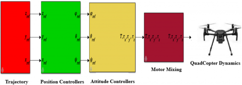
Simulink diagram
First, define the diagram of the quadcopter designed in Simulink (Table 2), providing an overview of each cascade in this diagram.
Table 2. Parameters of the quadcopter designed
|
Parameters |
Value |
|
Ixx |
0.09 $\mathrm{kg} / \mathrm{m}^2$ |
|
Iyy |
0.09 $\mathrm{kg} / \mathrm{m}^2$ |
|
Izz |
0.15 $\mathrm{kg} / \mathrm{m}^2$ |
|
m |
8 kg |
|
K |
0.0191 |
|
Ts |
0.01 s |
The Simulink diagram in Figure 11 illustrates a quadrotor design with six PID controllers for stability and responsiveness. These controllers manage position and altitude, ensuring the quadrotor follows a predefined trajectory and maintains a steady height. The position controller handles lateral movement, while the altitude controller adjusts vertical position. This setup allows for detailed analysis and optimization of the quadrotor's performance.
Figure 11. Schema of Simulink diagram
Trajectory
The trajectory is essential for simulating a drone's performance in agricultural missions. It involves the drone ascending to 5 meters and following a predefined path, moving 30 meters along the x-axis and 100 meters along the y-axis. This path provides clear guidance for evaluating the drone's real-world effectiveness as shown in Figure 12.
Figure 12. Trajectory given to follow
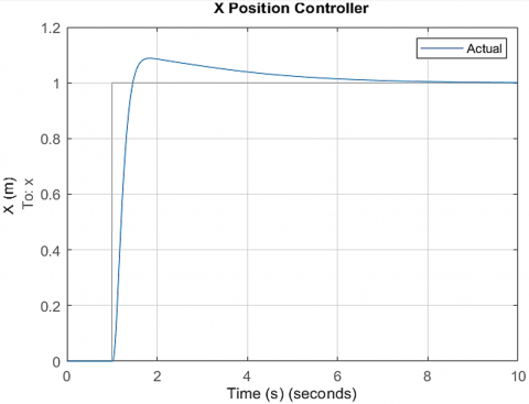
Position controllers
The position controller in a drone is crucial for maintaining precise positioning in three dimensions (Z Y X). It receives reference inputs for desired positions and calculates errors to adjust the drone's actuators, ensuring it maneuvers effectively to achieve the desired positions as shown in Figure 13.
Figure 13. Schema position controller
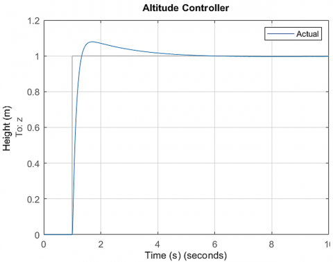
Altitude controller
To calculate errors between desired positions and actual measurements, adjusting actuators to achieve desired altitude and ensuring stability during flight as shown in Figures 14.
Figure 14. Schema altitude controller
4.12 Motor mixing
Motor mixing is a crucial process in multi-rotor drone control, determining power distribution among motors to achieve desired flight behavior as shown in Figure 15. It ensures stability by adjusting motor speeds based on control inputs like roll, pitch, and yaw angles.
Figure 15. Schema motor mixing
4.13 Quadcopter dynamics
In this section, the dynamics of a quadcopter are examined, with particular attention paid to input processing, output processing, and the six degrees of freedom (6DOF). It draws attention to the relationship that exists between the quadcopter's dynamics and the mathematical model and explains the importance that relationship is to understand and controlling flight behavior.
4.14 Result of simulation
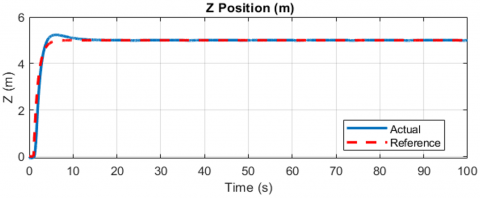
The initial section presents trajectory tracking results for the quadrotor along the X, Y, and Z axes. This analysis compares the actual and reference trajectories to evaluate the control system's accuracy and effectiveness. Figure 16 is a visual representation of the system's behavior in each dimension.
This examination evaluates the quadrotor system's performance in following a prescribed trajectory and maintaining stable flight. The chosen trajectory, shown in Figures 16 and 17, was simulated using MATLAB. Figure 16 compares the desired path (in blue) with the actual path followed by the drone (in red).
Figure 16. Quadcopter dynamics
Figure 17. The drone's trajectory along the X, Y, and Z axes and trajectory followed by drone
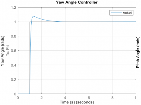
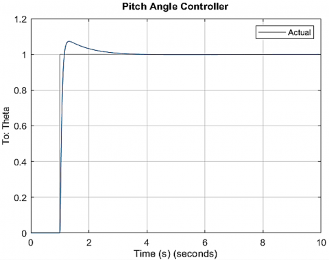
Figure 17 illustrates the comparison between the reference (in red) and actual (in blue) positions of X, Y, and Z, as well as the yaw pitch and roll angle Figure 16, when employing a PID controller.
4.15 PID controller response analysis
This section assesses the effectiveness of PID controllers in quadrotor system trajectory tracking, focusing on their contribution to accuracy and maintaining the desired path. Visual demonstrations and simulation results are provided in Table 3 and Figure 18.
Table 3. PID controller gain values
|
Gain |
$\boldsymbol{K}_p$ |
$\boldsymbol{K}_I$ |
$\boldsymbol{K}_D$ |
|
X |
-0.2 |
-0.01 |
-0.4 |
|
Y |
0.2 |
0.01 |
0.4 |
|
Z |
45 |
10 |
60 |
|
$\varphi$ |
5 |
1.5 |
3.5 |
|
$\theta$ |
5 |
1.5 |
3.5 |
|
$\psi$ |
3.5 |
1.5 |
2.5 |
(a)
(b)
Figure 18. Angle step input results and, position step input results and position step input results
Tuning the six parameters—X, Y, and Z for position control, and yaw, pitch, and roll for orientation control—ensures drone stability during flight. By adjusting these parameters within the PID controllers, the system effectively regulates the drone's position and orientation, minimizing oscillations and deviations from the desired trajectory.
Finally, the six PID controllers stabilize the drone, as evidenced by its ability to follow the prescribed path, simulating real-world conditions for spraying a square field. The 3D and 2D trajectory plots demonstrate how the drone accurately follows the given trajectory around the X, Y, and Z axes. The tuning of the PID controllers effectively regulates the drone's position and orientation, minimizing oscillations and deviations during flight.
The study aims to reduce the cost of spraying fields for farmers by using drones with multispectral cameras to detect plant diseases. Data is then analyzed using Pix4Dfields and Agremo software to assess crop yields and identify potential solutions. The research aims to achieve precision in spraying without excessive resource utilization.
5.1 Pix4Dfields analyzing
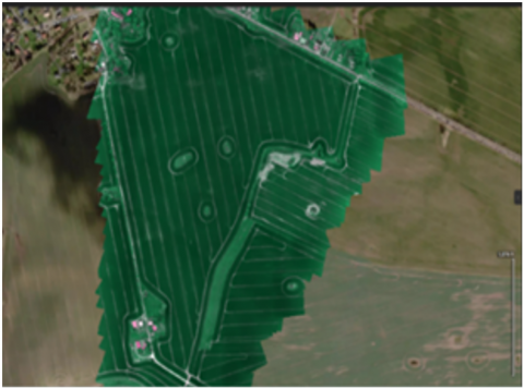
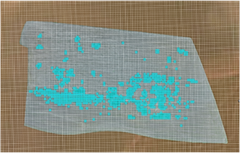
Pix4Dfields is a powerful agricultural mapping platform that, while effective, requires manual input for data analysis. The research involves an in-depth field examination using multispectral imagery to identify areas needing treatment and assess crop health. This analysis helps in pinpointing specific issues and determining the precise application of herbicides. The Figure 19 below illustrates a field used for practicing weed detection and targeting herbicide application, offering a comparison to traditional, less precise spraying methods.
The weed detection process using Pix4Dfields relies on sophisticated tools that allows users to identify weeds and automatically select all instances of them within the imagery. This tool facilitates the identification of areas requiring herbicide application to maintain crop health and optimize yield.
Using the magic tool from Pix4Dfield, we can measure the areas needing herbicide application and identify where weeds are present. Figure 19 shows the areas requiring spraying, marked by blue squares, indicating the locations where weeds have been detected.
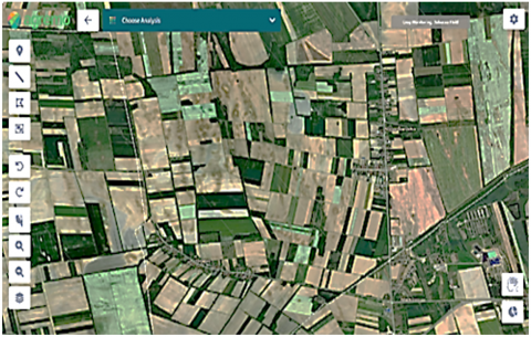
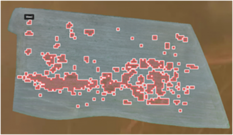
The Figure 20 illustrates weed detection and herbicide application in specific areas. Pix4Dfields aids in precise spot spraying by loading files directly onto the drone's interface, ensuring precision in agricultural operations, allowing seamless transfer to the drone's SD card.
Figure 19. Areas requiring herbicide application
Figure 20. Example field under examination
5.2 Analysis field in Agremo
Agremo is an AI-powered website that uses aerial imagery to create precise spraying maps, aiding in pesticide application and crop management strategies, particularly in monitoring sugar beet fields (Figure 21).
The analysis identifies stressed plants, assesses vigor, and detects waterlogging, providing crucial insights into crop health. This proactive approach enables targeted interventions for watering or pesticide application, optimizing crop yield. One key result from the analysis using advanced software is the stand count, offering valuable insights into crop density in the field. Figure 21 illustrates the results of this analysis.
Figure 21. Agremo result of field analysis using
The Agremo tool optimizes field spraying by analyzing variability, stress, and creating management zones, allowing drones to spray only areas needing treatment, minimizing herbicide use.
5.3 Impact of drones in agriculture
The impact of drones in agriculture can be evaluated by comparing budget costs, spraying area, and herbicide or pesticide costs, as shown in Table 4.
Figure 22 compares conventional flat spraying methods with drone spraying integrated with AI for analysis, highlighting the need for drones in fields with unhealthy crops.
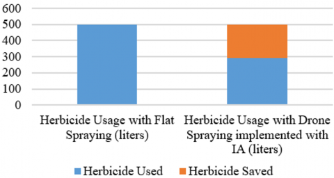
As farmers I have 500 litter of herbicide need to use it for spraying the field the diagram below shows the usage od herbicides for each case as shown in Figure 23.
After employing a total of 500 liters of herbicide sprayed using drones integrated with IA technology, there is a reduction of 210 liters compared to the standard herbicide pesticides usage with traditional flat spraying methods as shown in Figure 23.
Drones and advanced tools for weed detection can significantly reduce farmers' costs, with the cost per acre decreasing from $22 to $4.05. This is due to precision targeting, minimizing herbicide use, and optimizing resource allocation as shown in Figure 24.
Table 4. Cost comparison: flat spraying vs. AI and drone spraying
|
Coste of Spraying |
||
|
|
Flat Spraying |
DronePix4dfield Agremo |
|
Area sprayed(acres) |
65 |
|
|
Herbicide used per acre |
100% |
58% |
|
Herbicide cost per acre |
7.00$ |
4.06$ |
|
Total herbicide cost |
455.00$ |
263.00$ |
|
Yield losses from driving through the field per acre |
15.00$ |
0.00$ |
|
Total yield losses from driving through the field |
975.00$ |
0.00$ |
|
Total cost |
1430.00$ |
263.00$ |
Figure 22. Comparison of the area required for spraying
Figure 23. Usage of pesticides
Figure 24. Cost per acre
The drone employs an Arduino and pump system to precisely apply chemicals or water to specific locations, ensuring targeted and efficient application without waste.
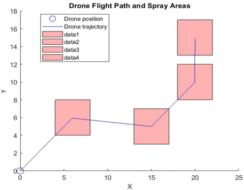
Finally, the research on drone-based pesticide spraying systems presents significant practical implications for agriculture. Equipping drones with a ground-connected tube allows for an unlimited pesticide supply, improving payload management and enabling continuous spraying without frequent recharges. This setup enhances operational efficiency and stability, with a support system mitigating the impact of the tube's weight. The integration of a multispectral camera for data collection further refines precision in pesticide application, targeting specific areas and reducing costs from \$22 to \$4.05. Additionally, this approach mitigates the adverse effects of traditional farming methods, such as human health risks from pesticide exposure and soil degradation [25]. UAVs help minimize these risks by applying pesticides more accurately, thereby reducing overall chemical use. However, challenges such as deployment reliability, equipment maintenance, and data management must be addressed to optimize UAV technology in agriculture and promote sustainable, cost-effective farming practices (Figure 25).
Figure 25. Drone flight path and spray areas
This study shows the value of quadcopter technology in agriculture and how it may effectively address the problems faced by farmers. A quadcopter with a sturdy structure for carrying heavy loads and an assortment of parts including the TM5212 engine and 15*5CF propeller was designed with SolidWorks 2022 to spray water and pesticides over wide areas. SolidWorks simulations validated the drone's robustness and capacity to do agricultural tasks. MATLAB Simulink simulations evaluated component response and trajectory tracking, offering important information into the drone's performance and the efficacy of the chosen parts.
These simulations provide valuable insights into the drone's capabilities and the effectiveness of the selected components for agricultural missions. Additionally, to further optimize pesticide usage and boost farmers' profits, the drone will utilize a multispectral camera for mapping purposes. This camera will capture data during flight, which will then be analyzed using software like PIX4D and Agremo. These advanced tools enable precise analysis of the collected data, allowing us to identify specific areas in the field that require spraying. By integrating this technology with the drone's capabilities, we can ensure targeted and efficient pesticide application, minimizing waste while maximizing crop health and profitability for farmers.
Despite promising results, challenges in deployment, maintenance, and operation in real agricultural settings remain. The next phase involves creating a drone that can continually access pesticides through a tube from a ground-based source, eliminating the need for refilling. This aims to maximize the drone's utility and impact in agriculture by balancing an endless supply of pesticides with longer flight durations, allowing the drone to cover wide areas for spraying missions without interruption. Additionally, research into more efficient battery technologies or alternative power sources, such as solar panels, can extend drone flight times and reduce the frequency of recharging. Enabling multiple drones to operate in a coordinated swarm can increase coverage area and efficiency, particularly for large-scale farming operations. Furthermore, designing drones with improved weather resistance can ensure reliable operation in various environmental conditions, enhancing their utility in diverse agricultural settings.
|
$R_z(\psi)$ |
Rotation Matrix for Rotation about Z-Axis |
|
$R_y(\psi)$ |
Rotation Matrix for Rotation about Y-Axis |
|
$R_x(\psi)$ |
Rotation Matrix for Rotation about X-Axis |
|
$T_I^B$ |
Rotation from a Body-Fixed B Frame to an Inertial Frame I |
|
$V 1$ |
Linear Velocities in the Inertial Frame, m/s |
|
$m$ |
The Mass of Rigid Body, g |
|
$F_B$ |
External Force, N |
|
$M_B$ |
External Moment, N/m |
|
$I$ |
Moment, kg.s-2 |
|
$F_M$ |
Force Generated by Motors, N |
|
$F_G$ |
Force Gravitational, N |
|
$F_W$ |
Force Exerted by Wind, N |
|
$M_M$ |
Moment Generated by Motors, N.m |
|
$M_G$ |
Moment Gravitational, N.m |
|
$M_W$ |
Moment Exerted by Wind, N.m |
|
$K_p$ |
Proportional Gain |
|
$K_D$ |
Derivative Gain, s |
|
$K_I$ |
Integral Gain s-1 |
|
$e(t)$ |
The Error Term |
|
$u(t)$ |
The Control Input |
|
Greek symbols |
|
|
$\lambda$ |
Linear Position, m |
|
$\eta$ |
Euler Angles, rad |
|
$\omega_E$ |
Euler Angle Rates in the Inertial Frame, rad/s |
[1] Lai, J., Ford, J.J., Mejias, L., O'Shea, P., Walker, R. (2012). See and avoid using onboard computer vision. Sense and Avoid in UAS: Research and Applications, 265-294. https://doi.org/10.1002/9781119964049.ch10
[2] Chamola, V., Kotesh, P., Agarwal, A., Gupta, N., Guizani, M. (2021). A comprehensive review of unmanned aerial vehicle attacks and neutralization techniques. Ad Hoc Networks, 111: 102324. https://doi.org/10.1016/j.adhoc.2020.102324
[3] Ma, L., Li, M., Tong, L., Wang, Y., Cheng, L. (2013). Using unmanned aerial vehicle for remote sensing application. In 2013 21st International Conference on Geoinformatics, Kaifeng, China, pp. 1-5. https://doi.org/10.1109/Geoinformatics.2013.6626078
[4] Mogili, U.R., Deepak, B.B.V.L. (2018). Review on application of drone systems in precision agriculture. Procedia Computer Science, 133: 502-509. https://doi.org/10.1016/j.procs.2018.07.063
[5] Mohsan, S.A.H., Othman, N.Q.H., Li, Y., Alsharif, M.H., Khan, M.A. (2023). Unmanned aerial vehicles (UAVs): Practical aspects, applications, open challenges, security issues, and future trends. Intelligent Service Robotics, 16(1): 109-137. https://doi.org/10.1007/s11370-022-00452-4
[6] Matthews, G. (2015). Pesticides: Health, Safety and the Environment. John Wiley & Sons.
[7] Pathak, V.M., Verma, V.K., Rawat, B.S., Kaur, B., et al. (2022). Current status of pesticide effects on environment, human health and it’s eco-friendly management as bioremediation: A comprehensive review. Frontiers in Microbiology, 13: 962619. https://doi.org/10.3389/fmicb.2022.962619
[8] Hanif, A.S., Han, X., Yu, S.H. (2022). Independent control spraying system for UAV-based precise variable sprayer: A review. Drones, 6(12): 383. https://doi.org/10.3390/drones6120383
[9] Ju, C., Son, H.I. (2018). Multiple UAV systems for agricultural applications: Control, implementation, and evaluation. Electronics, 7(9): 162. https://doi.org/10.3390/electronics7090162
[10] Bouabdallah, S., Noth, A., Siegwart, R. (2004). PID vs LQ control techniques applied to an indoor micro quadrotor. In 2004 IEEE/RSJ International Conference on Intelligent Robots and Systems (IROS) (IEEE Cat. No.04CH37566), Sendai, Japan, pp. 2451-2456https://doi.org/10.1109/IROS.2004.1389776
[11] Oersted, H., Ma, Y. (2023). Review of PID controller applications for UAVs. arXiv preprint arXiv:2311.06809. https://doi.org/10.48550/arXiv.2311.06809
[12] Salim, N.D., Derawi, D., Abdullah, S.S., Mazlan, S.A., Zamzuri, H. (2014). PID plus LQR attitude control for hexarotor MAV in indoor environments. In 2014 IEEE International Conference on Industrial Technology (ICIT): Busan, Korea (South), pp. 85-90. https://doi.org/10.1109/ICIT.2014.6894977
[13] Suprapto, B.Y., Heryanto, M.A., Suprijono, H., Muliadi, J., Kusumoputro, B. (2017). Design and development of heavy-lift hexacopter for heavy payload. In 2017 International Seminar on Application for Technology of Information and Communication (iSemantic), Semarang, Indonesia, pp. 242-247. https://doi.org/10.1109/ISEMANTIC.2017.8251877
[14] Phang, S.K., Cai, C., Chen, B.M., Lee, T.H. (2012). Design and mathematical modeling of a 4-standard-propeller (4SP) quadrotor. In Proceedings of the 10th World Congress on Intelligent Control and Automation, Beijing, China, pp. 3270-3275. https://doi.org/10.1109/WCICA.2012.6358437
[15] Carev, V., Roháč, J., Šipoš, M., Schmirler, M. (2021). A multilayer brushless DC motor for heavy lift drones. Energies, 14(9): 2504. https://doi.org/10.3390/en14092504
[16] Assmann, J.J., Kerby, J.T., Cunliffe, A.M., Myers-Smith, I.H. (2018). Vegetation monitoring using multispectral sensors—best practices and lessons learned from high latitudes. Journal of Unmanned Vehicle Systems, 7(1): 54-75. https://doi.org/10.1139/juvs-2018-0018
[17] Kopačková-Strnadová, V., Koucká, L., Jelének, J., Lhotáková, Z., Oulehle, F. (2021). Canopy top, height and photosynthetic pigment estimation using parrot sequoia multispectral imagery and the unmanned aerial vehicle (UAV). Remote Sensing, 13(4): 705. https://doi.org/10.3390/rs13040705
[18] Akkoyun, F. (2019). Design and development of an unmanned aerial and ground vehicles for precision pesticide spraying. Doctoral thesis, Adnan Menderes Üniversitesi Fen Bilimleri Enstitüsü.
[19] Suresh, H., Sulficar, A., Desai, V. (2018). Hovering control of a quadcopter using linear and nonlinear techniques. International Journal of Mechatronics and Automation, 6(2-3): 120-129. https://doi.org/10.1504/IJMA.2018.094488
[20] Junkins, J.L., Shuster, M.D. (1993). The geometry of the Euler angles. Journal of the Astronautical Sciences, 41(4): 531-543.
[21] Depriester, D. (2020). Computing Euler angles with Bunge convention from rotation matrix. https://www.researchgate.net/profile/Dorian-Depriester/publication/324088567_Computing_Euler_angles_with_Bunge_convention_from_rotation_matrix/links/5faa9190458515157bfc2650/Computing-Euler-angles-with-Bunge-convention-from-rotation-matrix.pdf.
[22] Mohamed, K.S. (2018). Machine Learning for Model Order Reduction (Vol. 664). Berlin, Germany: Springer.
[23] Covic, N., Salihbegovic, A. (2023). The state-space representation of MIMO LTI systems using the future inputs elimination approach. In 2023 9th International Conference on Control, Decision and Information Technologies (CoDIT), Rome, Italy, pp. 1589-1594. https://doi.org/10.1109/CoDIT58514.2023.10284180
[24] Altalabani, W., Alaiwi, Y. (2022). Optimized adaptive PID controller design for trajectory tracking of a quadcopter. Mathematical Modelling of Engineering Problems, 9(6): 1490-1496. https://doi.org/10.18280/mmep.090607
[25] Ahmad, M. F., Ahmad, FA., Alsayegh, A.A., Zeyaullah, M., et al. (2024). Pesticides impacts on human health and the environment with their mechanisms of action and possible countermeasures. Heliyon, 10(7): e29128. https://doi.org/10.1016/j.heliyon.2024.e29128