Sushma Parihar![]() | Pritesh Shah*
| Pritesh Shah*![]() | Ravi Sekhar
| Ravi Sekhar![]() | Kalyani Bhole
| Kalyani Bhole![]()
© 2025 The authors. This article is published by IIETA and is licensed under the CC BY 4.0 license (http://creativecommons.org/licenses/by/4.0/).
OPEN ACCESS
Healthcare jobs are facing large shortages. It is imperative to explore feasible technological solutions to ease the burden of healthcare professionals. This paper presents a model predictive control (MPC) design to suggest a suitable anesthetic drug delivery rate to attain the desired level of sedation prescribed by an anesthesiologist for patients undergoing surgical procedures. This controller was designed on a detailed pharmacokinetics model that accounted for anesthetic drug inhalation, exhalation, excretion, as well as absorption and circulation through different tissue groups such as brain, lungs, heart, kidneys, liver, muscles, and fats. The proposed MPC controller was tuned under different conditions such as constant setpoint, temporally varying setpoints, and noise signal disturbances to simulate real-world scenarios. A proportional integral derivative (PID) controller was also tuned for all above-mentioned conditions for performance comparisons. Primary results of output signals (resultant drug concentration in the patient body) showed that the PID controller achieved lower settling times, whereas MPC minimized overshoots more effectively in all conditions. The difference between the settling times of MPC and PID was less than 1.5 seconds in all cases except for noise disturbances, wherein the maximum settling time was about 18 seconds for the best performing MPC architecture. A delay of 18 seconds in achieving the required anesthetic drug concentration in the patient body is not as detrimental compared to the risks of suggesting a drug delivery rate that leads to anesthetic overdosage. Hence, this study shows that suggestive MPC controllers can be considered in surgical anesthetic drug delivery applications for assisting anesthesiologists.
model predictive control, PID, anesthesia, pharmacokinetics, surgery, suggestive controller, drug delivery
Strong inadequate demand for healthcare professionals is not new in the health system. The scarcity of healthcare human capital has been a well-established problem for many developed and developing countries for several years [1]. Several techniques have been reported to address the current and future global healthcare workforce demands [2]. Scientists also have sought to find different approaches and methods of combining the traditional modeling-based automated solutions to certain trends related to bio-medical fields [3]. The aim of these researchers was to develop improved statistical models with a view of aiding clinical diagnosis and therapeutic management. Biological processes are nonlinear and time varying in nature, this makes the process of studying and controlling the related biology very difficult. However, the positive closed loop architectures can be designed to recommend appropriate actions for achieving the intended treatment regulation. The fractional order models are far better in system identification and control precision than the integer order models and for that these have been found more suitable for the anesthesia management [4, 5]. The MPC approach is implemented as an LMI-based predictive control method to regulate a single-chamber microbial fuel cell (MFC) system with the primary goals to shorten the time to reach steady-state, minimize system error, and ensure closed-loop stability [6]. MPC techniques are well-suited for applications requiring robust control of constrained, multivariable processes [7]. Likewise, system identification and control systems can also be employed for the support of medical operations as well. More researchers are implementing the concepts of biomedical control engineering [8]. Closed-loop controls in biomedicines can be translated into useful and reproducible systems. Recent studies on event-based model predictive control (MPC) for anesthesia control show diminished control signal variations and propofol usage, at the cost of slightly lower control performance. These systems have been found to be resistant to patient variability and noise to satisfactory clinical standards as have been noted [9, 10]. Also, integrating MPC with event-based PID controllers for Depth-of-Hypnosis (DoH) for total intravenous anesthesia (TIVA) may stand to enhance mimic the behaviour of the anesthetist, enabling faster induction and enhanced control [11].
The healthcare sensor systems in the modern world can be utilized to transform the clinical health results into quantitative control parameters. The receding horizon control techniques of MPCs are well suited for the control of medicine distribution. MPCs have been sighted to achieve stable performance in medical applications [12]. This work provides MPC controller formulations for recommending appropriate anesthetic drug dosing rates to achieve the level of sedation that is required for patients under surgical procedures.
The exact regulation of anesthesia depth while reducing the risk of overdose persists as a challenge, even with the developments in anesthetic drug delivery systems. The fluctuating physiological state of patients are frequently not accommodated by current approaches. To address these issues, this work presents a model predictive control (MPC) system built on a thorough pharmacokinetics model. The goal of the study is to demonstrate the benefits and distinctive contributions of the suggested method by including noise disturbances and contrasting the MPC with a conventional PID controller.
PID control benefits medical systems in a number of ways. First off, it's a flexible option for controlling intricate physiological indicators like mean arterial pressure (MAP) due to its broad application and ease of use. Furthermore, as shown in the example of fractional-order PID controllers for MAP regulation, PID controllers can be optimized using methods like genetic algorithms, leading to better performance metrics in comparison to alternative control schemes [13]. Moreover, PID controllers' versatility enables efficient regulation in changing medical settings, as demonstrated by their excellent application in closed-loop drug delivery systems to reduce persistent nonlinear oscillations in the neuromuscular blockade (NMB) system [14]. PID control does, however, have several drawbacks when used in medical settings. EEG-based propofol dosage control illustrates how the inherent linearity assumption might make it challenging to achieve optimal control performance and dose accuracy [15]. PID parameters are hard to tune, especially in nonlinear systems like magnetic nanofluid hyperthermia for cancer treatment [16], emphasizing the need for more complex control techniques to solve these constraints and increase patient safety.
Based on MPC, the paper offers a method that implies the optimal rate of anesthetic medication delivery. Predicting behavior based on a dynamic model of the system helps MPC, an advanced control technique, maximize control operations across a restricted time horizon. Over standard control methods, the new use of MPC to anesthetic medication delivery in real-time surgical environments shows possible advantages. The design of the MPC controller is derived from a pharmacokinetic model including the rates of drug exhalation and excretion as well as the rates of drug transmission amongst several tissue groups in the human body. This whole model, which captures the complex dynamics of medication distribution and elimination over the body, enhances the precision of control decisions. The MPC controllers are tuned to lower overshoots and undershoots in the drug concentration levels of the patient. When the system is fine-tuned, safe and stable drug amounts are kept even when setpoints are disrupted or changed. Compared to an auto-tuned PID controller, the study investigates how well MPC controllers’ function in several situations. As this comparison study reveals, MPC should limit output overshoots if we are to lower the likelihood of anesthetic overdosage. Research indicates that for guiding the delivery of anesthetic medications in real-world clinical environments, MPC systems could be a safer alternative than PID controllers. The paper underlines how adding MPC-based control systems into anesthetic delivery systems might improve surgical performance and patient results. The study enhances the field of anesthetic control generally by offering a novel approach using pharmacokinetic modeling and MPC to maximize drug distribution and enhance patient safety during surgery. MPC and its function in anesthetic operations are briefly introduced in the section that follows.
1.1 Model predictive control
MPC is a group of computer control approaches that are used to develop explicit models of plant processes in order to accurately predict the relevant responses. It is an effective method for dealing with plants involving multivariable control. MPC was initially developed for controlling nonlinear dynamic systems having multiple constrained inputs and outputs in the chemical processing industries [17]. MPC can regulate plant outputs while permitting online input-output process exchanges. MPC can also handle complex plants involving conflicting regulations. MPC can preemptively analyze information and respond appropriately to the actual plant outputs. In the early 1960s, MPC pioneers worked on few isolated industry applications [18]. De Keyser et al. [19] studied self-adaptive long-range predictive control (LRPC) approaches in 1988, whereas Garcia et al. [18] reviewed linear quadratic MPC control architectures. Scattolini and Bittanti [20] explored the impulse/plant step prediction horizons. Clarke and Scattolini [21] stabilized general linear plants using quadratic function optimization over a costing horizon. Qin and Badgwell [22] reviewed commercial MPC technologies. Jalali and Nadimi [23] investigated MPC robustness, constraints-handling, stability and performance aspects. Warren and Marlin [24] designed an MPC architecture that assessed closed-loop uncertainty of input constraints to ensure resilient process outputs. Others evaluated MPC performance and disturbance uncertainties [25].
1.1.1 MPC implementation
MPC implementation requires current process data, dynamic parameters, output setpoint targets, and tolerances [26]. The model constraints for the dependent and independent variables are used to regulate the MPC parameters. In an MPC-controlled system, independent variables affect dependent variables and MPCs can be linear or nonlinear and explicit or robust [27]. Linear MPCs can predict dependent variable responses by integrating the effects of many independent factors. The control problem is thus reduced to a series of quick and dependable linear matrix algebra calculations. After developing the linear MPC model, several process variables can be corrected for nonlinear system behaviors. Nonlinear MPC models can directly control such systems. Nonlinear MPC models could be built on energy and mass balance fundamentals or empirical relations based on data (e.g., artificial neural networks). Linearizing a nonlinear model produces a linear MPC or Kalman filter [28]. Nonlinear model predictive control (NMPC) uses a nonlinear dynamic model and nonlinear constraints. Both linear and nonlinear MPCs require several iterations within the prediction horizon to find the optimal control parameters [29, 30]. Industrial processes with slow sample rates or scattered parameter systems generally use NMPC models. Recent advances in computing methods and controller technology have enabled large-scale implementations of NMPCs in high-sampling-rate applications like automobile manufacturing and aeronautical applications [31]. Unlike online MPCs, explicit MPCs (eMPCs) provide faster control rule evaluations [32]. Piecewise affine functions represent this offline pre-computed solution (PWA). The eMPC controller preserves piecewise affine function coefficients for constant state spaces and stores the state space parametric coefficients for further processing.
1.1.2 MPC merits
Due to the advancements in computing technologies, MPCs are now capable of being applied to processes that are more dynamic, whereas earlier they could only be used for slow and steady processes. An MPC is able to handle restrictions in an effective manner. It is also relatively simpler to adapt and tailor to one’s specific needs. In MPC, it is possible to establish limitations not only on the output of controlled processes (the control variable), but also on the control signals that are inputs to the controlled processes.
Input restrictions can take the form of rate constraints such as in the case of valves and other actuators. MPC also performs better than traditional controllers in situations where the process has a large number of linear/nonlinear constraints. MPCs are ideally suited for systems involving structural changes, unstable processes and non-minimal phases. The next section introduces anesthesia and the related role of MPC.
1.2 Anesthesia and MPC
Anesthesia is required in surgeries, dental procedures and intensive care. Anesthesia puts patients under se- dation to make operations painless. Anesthesia comprises of three phases: induction, maintenance, and emergence. Anesthetic drugs include propofol, remifentanil, sevoflurane, isoflurane, desflurane among others. Anesthetic underdosage causes patient awareness of the operation, whereas overmedication can also potentially harm the patient’s body. Thus, one of the most difficult medical duties is maintaining the optimal degree of sedation during and after anesthetic induction. Suggestive regulation of total intravenous anesthesia is crucial due to the high number of procedures performed daily worldwide [33]. Challenges such as increased clinical burden, diverse infusion methods and repetitive use of a consistent infusion rate can be overcome by using controller based suggestive drug delivery rates.
Anesthesia control necessitates robustness to disturbances and avoidance of overdosage to minimize adverse pharmacokinetic and pharmacodynamic interactions. Computer-controlled automatic perfusion syringes can administer intravenous anesthesia and painkillers. Parameters such as BIS index and EEG signal entropy are used to measure the depth of anesthesia [34]. Researchers used an in situ model to build a control loop to distribute remifentanil and propofol in patient body using a pharmacokinetic-dynamic model that replicated patients’ in situ bio-responses such as heart rate and arterial pressure. Another study used a single input (propofol infusion rate) and single output (bispectral index) model to study the relationship between anesthetic dose and the resultant hypnotic effects [35]. The authors used MPC to control BIS index subjected to the bio-medical parameter constraints and restrictions. In another study, researchers devised an MPC-based feedback controller with a time-delay-handling feature to improve anesthesia [36]. Researchers agree that computer-controlled/suggested infusion systems help maintain the positive balance between underdosage and over infusion of anesthetic drugs [37]. Computer-controlled/suggested drug delivery handles routine chores like anesthetic and hemodynamic maintenance so that medical personnel can spare attention to other critical tasks. Suggestive clinical anesthetic automation is driven by patient safety and offers many benefits:
·Prevention of under/overdosage.
·Cost savings through optimal drug delivery.
·Decision support in the form of a suggested drug infusion rate.
·Reduced dependency on highly skilled/experienced anesthesiologists for general cases.
In the conventional medication regime, an anesthesiologist sets the initial dosage set point targets and adjusts them based on the patients’ depth of anesthesia and bio-responses. Generally, anesthesiologists estimate pharmaceutical responses based on the available monitoring equipment, clinical judgment and experience. However, closed-loop automated control systems can promptly suggest suitable medication infusion rates based on the pharmacokinetic models of anesthetic drug concentrations actually absorbed by the patient body. The following section provides details of the pharmacokinetic modeling adopted in the present study.
This section firstly introduces pharmacokinetics, pharmacodynamics and the anesthetic drug considered in the present work: sevoflurane. Secondly, it presents the human body compartmentalization and pharmacokinetics based anesthetic modelling procedure. Thirdly, it explains how this model was implemented in the present work.
2.1 Pharmacokinetics, pharmacodynamics and sevoflurane
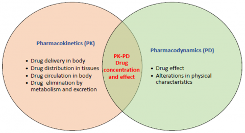
Pharmacokinetics refers to a modeling approach that depicts how man-made or naturally occurring chemical compounds are absorbed, distributed, metabolized, and eliminated by human beings and/or animal species. On the other hand, in pharmacodynamic investigations, a medication is administered, and the effect is assessed by drawing blood at various times to estimate the amount of drug that was present in the blood at the time that the effect was observed. Body parameters such as blood pressure, heart rate, and other parameters alter because of the action of the medicine. Parameters of pharmacokinetics and pharmacodynamics characterize the behavior of the hypnotic medication. Distribution of the drug, metabolism, absorption of the drug and elimination are some of the time-dependent physiologic processes that are controlled by the pharmacokinetic parameters after infusion [38]. On the other hand, the pharmacodynamic parameters control blood concentration of the drug and its effect at the intended site [39]. Both the pharmacokinetics and the pharmacodynamics are related to one another, as shown in Figure 1.
In pharmacokinetics, an anesthetic drug is introduced into the patient’s body by an injection or inhalation. The injected/inhaled drug is absorbed by lungs and circulated throughout the body tissues. Subsequently, the anesthetic drug passes through metabolism before it is finally eliminated from the body (excretion). In accordance with the principles of pharmacodynamics, the anesthetic drug will not begin to exert its effects until after it has altered metabolic processes within the body, such as the pace at which the heart beats and the blood pressure. The sevoflurane anesthetic drug is a transparent, colorless and volatile liquid that can be vaporized and inhaled. Sevoflurane stands out from other inhalational agents because it is barely soluble in blood. A combination of nitrous oxide and oxygen is commonly used for delivering this anesthetic to patients undergoing surgery. Sevoflurane, being almost insoluble and biodegradable, is eliminated from the body more rapidly as compared to other anesthetic drugs [11].
Anesthesia modelling based on human body compartmentalization and pharmacokinetics: Medical researchers separate the human body into several sections based on the blood circulation to different compartments [40]. This compartmental model is a simple kinetics framework for describing drug absorption, distribution, excretion and is widely utilized in many different biomedical contexts due to its adaptability and ease of use in relating pharmacokinetic drug levels to pharmacodynamic markers [41]. As shown in Figure 2 [42], the drug is distributed according to a pharmacokinetic model having five compartments.
Figure 1. Pharmacokinetics/pharmacodynamics interactions
Figure 2. Five compartmental model of pharmacokinetics
When the anesthetic drug is inhaled by the patient, it is firstly absorbed by the lungs, labelled as the compartment (C1). The absorbed drug in the blood stream is circulated to different tissue groups such as the brain, lungs, heart, kidneys and liver (C2), the muscle groups (C3), the fats that surround the vessel rich organs (C4) and the fat groups in general (C5). The drug is eliminated from the body via lungs and kidneys, whereas drug-response metabolic processes take place in the C2, C3, C4, and C5 compartments. k12, k13, k14 and k15 represent the intercompartmental drug transfer s from C1 (lungs) to all other compartments. Conversely, k21, k31, k41 and k51 represent the intercompartmental drug transfer rate constants from all compartments to C1. k10 and k20 represent the drug excretion rate constants from compartments C1 and C2 respectively. These constants are also known as the mammalian rate constants. The present study builds upon the pharmacokinetics and human body compartmentalization-based anesthesia model developed by Dhandore et al. [11] for the Sevoflurane drug, wherein they did not consider the effect of drug exchanges between the C4 and C5 compartments with the C1 compartment to determine the rate of change of drug concentration at C1. The present study factored in the drug interactions between C4-C1 and C5-C1 as well. Furthermore, the said authors only specified drug delivery at C1, whereas the present work specified the rate of drug delivery at C1 for a better correlation against the expected output of the rate of change of drug concentration in C1. Following is the resultant anesthesia model based on the pharmacokinetic interactions occurring in the human body compartments (Figure 2).
$\begin{gathered}\frac{d x_1}{d t}=\frac{d}{d t}( { inSev })-\left[\left(k_{10}+k_{12}+k_{13}+k_{14}+k_{15}\right) *\right. x_1+\left[k_{21} * x_2+k_{31} * x_3+k_{41} * x_4+k_{51} * x_5\right]\end{gathered}$ (1)
where, inSev indicates drug delivery, i.e., the Sevoflurane drug concentration (volume percentage) administered to the patient. xi indicates the volume percentage of Sevoflurane drug present in the ithcompartment. dx1/dt is the rate of change of Sevoflurane volume percentage in compartment C1 (lungs), which also indicates the net Sevoflurane drug concentration absorbed by the body. It is equal to total drug delivered to the patient (inSev), minus the total drug transmitted from lungs to other compartments, plus the total drug re-transmitted from those compartments back to the lungs. The rate of change of Sevoflurane volume percentages present in compartments C2, C3, C4 and C5, or in other words, the net Sevoflurane drug concentration absorbed by compartments C2, C3, C4 and C5 are expressed as follows:
$\begin{gathered}\frac{d x_2}{d t}=k_{12} * x_1-\left(k_{20}+k_{21}\right) * x_2 \\ \frac{d x_3}{d t}=k_{13} * x_1-k_{31} * x_3 \\ \frac{d x_4}{d t}=k_{14} * x_1-k_{41} * x_4 \\ \frac{d x_5}{d t}=k_{15} * x_1-k_{51} * x_5\end{gathered}$ (2)
2.2 Implementation
The tuning process for a model predictive controller (MPC) begins with selecting the sampling time and response speed metrics. The system is then discretized using the chosen sampling time, and constraints are defined for the inputs and manipulated variables. Next, MPC parameters are selected, and the model response is generated based on the plant input data and the specified output setpoint. The model estimation error is calculated as the cost function, and iterative adjustments are made to minimize this error. If the estimation error remains high after a significant number of iterations, the initial parameters—sampling time, response speed, and variable constraint are adjusted accordingly [7].
The MPC implements the following linear model for control [43]:
$\dot{a}(t)=K X(t)+L U(t)$ (3)
$b(t)=M X(t)+N U(t)$ (4)
where, X(t) represents the system's state, B(t) denotes the system's output, and U(t) is the system's input. The matrices K, L, M, and N are associated with the state-space model. For a control horizon of C steps, the optimal function at time t is expressed as [2]:
$H_{\min }=\sum_{\tau=t+1}^{t+C}(b(\tau))^2+r(u(\tau)-u(\tau-1))^2$ (5)
Subjected to $|u(\tau)| \leq u_0$ (6)
where, C represents the control horizon. The above equation provides the optimal control signal adjustments for the system's plant. The MPC controller predicts the system's output over (i-step), as shown in the following equation:
$B_i(t)=P X(t)+Q U_i(t)+G u(t)$ (7)
where, u(t) is computed based on the previous state, with the predicted output (Bi(t)) and the future control signal (Ui(t)) expressed as:
$b_i(t)=\left[\begin{array}{c}b(t+1) \\ b(t+2) \\ \vdots \\ b(t+i)\end{array}\right] ; U_i(t)=\left[\begin{array}{c}U(t+1) \\ U(t+2) \\ \vdots \\ U(t+i)\end{array}\right]$ (8)
The matrices P, Q and G are given by:
$P=\left[\begin{array}{c}M K \\ M K^2 \\ \vdots \\ M K^i\end{array}\right]$
$Q=\left[\begin{array}{cccc}0 & 0 & \ldots & 0 \\ C B & 0 & \ldots & 0 \\ \vdots & \vdots & \ddots & \vdots \\ M K^{i-2} L & M K^{i-3} L & \ldots & 0\end{array}\right]=\left[\begin{array}{cccc}j(1) & 0 & \ldots & 0 \\ j(2) & j(1) & \ldots & 0 \\ \vdots & \vdots & \ddots & \vdots \\ j(p) & j(i-1) & \ldots & j(1)\end{array}\right]$ (9)
$G=\left[\begin{array}{c}j(2) \\ j(3) \\ \vdots \\ j(i+1)\end{array}\right]$
Table 1 shows the mammillary rate constant.
MPC and its tuning were implemented on the model across various conditions. The tuning process involved adjusting several control parameters, including timestep, control and prediction horizons, as well as input and output constraints. The result of the tuning process revealed several findings. Notably, MPC crashed when the lower bound of the input was set to zero. Additionally, altering the upper bound of the input to infinity and the lower bound of the output to negative infinity did not yield any evident changes in the results. Similarly, there were no significant changes in the outcomes when the prediction and control horizons were varied by plus minus 50 percent.; however, the MPC encountered crashes if the horizons were adjusted beyond that range. Furthermore, the MPC malfunctioned when the timestep was set at 0.01 or below. Finally, the following bounds were selected as shown in the Table 2.
Out of all the controller designs that are currently accessible, the PID controllers are the ones that are most used.
$C(s)=K_p+K_I\left(\frac{1}{s}\right)+K_D\left(\frac{N}{1+N\left(\frac{1}{s}\right)}\right)$ (10)
where, $K_p$ represents the proportional gain, $K_I$ is the integral gain, $K_D$ is the derivative gain, and N is the filter coefficient for the derivative. The PID controller was auto-tuned using the time-domain methodology within the Simulink block (MATLAB) [44]. The auto-tuning process involved iterative adjustments of the PID parameters to achieve optimal controller performance. Table 3 presents the design parameters for the PID controller.
Table 1. Mammillary rate constant (min-1) [45]
|
Rate Constant |
Sevoflurane |
|
k10 |
1.78 ± 0.17a |
|
k12 |
0.709 ± 0.145a |
|
k13 |
0.223± 0.035a |
|
k14 |
0.125± 0.056a |
|
k15 |
0.0310± 0.0196a |
|
k21 |
0.194±0.092 |
|
k31 |
0.0231±0.0198 |
|
k41 |
0.00313±0.00180 |
|
k51 |
0.000502±0.000117 |
|
k20 |
0.0094±0.0171 |
Table 2. MPC controller designed parameters
|
Prediction horizon |
10 |
|
Control horizon |
2 |
|
Input constraint |
- infinity to 99.9 |
|
Output constraint |
0 to infinity |
Table 3. PID controller parameters
|
KP |
-25.51225205 |
|
KI |
-10.0025518 |
|
KD |
-5.952322713 |
|
N |
81.38036922 |
This model was implemented in MATLAB Simulink to be controlled by the MPC and PID controllers at prescribed set points for suggesting the required drug delivery rates. The mammalian rate constants for the Sevoflurane drug transfer were obtained from the study conducted by Yasuda et al. [42] wherein the authors administered 1% inhaled Sevoflurane with 34% oxygen and 65% nitrous oxide to a group of male patients aged 20-26 years, heights 175 to 189 cms and weighing 63 to 81 kg. The control system experiments were carried out in three categories: constant setpoint, constant setpoint with noise disturbances and varying setpoint conditions. The constant setpoint was selected at 1.6 volume percentage of net Sevoflurane drug concentration in lungs, as prescribed in literature [46]. In the second category, disturbances of 0.01 and 0.001 magnitudes were added to the closed loop with the same constant setpoint of 1.6, in order to test the controllers against possible signal disturbances occurring in actual application scenarios. The third category included three kinds of set- point variations, to test the controllers for scenarios wherein the anesthesiologist may change her/his decision of selecting the appropriate drug concentration required for a particular patient. Firstly, the setpoint was varied from 1.6 (0 to 4 seconds), 1.85 (4 to 6 seconds) to 1.7 (6 to 20 seconds). Second variation of setpoint was designed as 1.6 (0 to 6 seconds), 1.85 (6 to 16 seconds) and 1.7 (16 to 20 seconds). The third setpoint variation was designed as 1.6 (0 to 2 seconds), 1.85 (2 to 3 seconds) and 1.7 (3 to 20 seconds). Hence, the MPC and PID controllers were thoroughly tested under different conditions to investigate and validate their ability to control the given anesthetic model with desired accuracy and suggest the required drug delivery rates in every case. Figure 3 shows the generalized Simulink block diagram for the MPC/PID anesthetic drug flow rate suggestive controllers and Figure 4 shows the anesthesia sub system diagram. The PID controller was auto tuned in every case. The MPC controllers were tuned manually in terms of their lower/upper bounds, prediction/control horizons, and solution timesteps.
Figure 3. Block diagram
Figure 4. Anesthesia subsystem diagram
The objective of manual MPC tuning was to obtain the best controller parameters that allowed minimal settling time and under/overshoots. Minimal settling time of control signal would ensure quick response from the controller to the anesthesiologist regarding the suggested drug delivery rate for the desired drug concentration set point specified by her/him. Minimal settling time of output signal would ensure quick sedation of the patient with the required concentration of anesthetic in patient body. Minimal over and undershoots in the control signal would ensure minimal excess or insufficient delivery of Sevoflurane to the patient. Correspondingly, minimization of over and undershoots in output signal would ensure minimal excess or insufficient concentration of Sevoflurane actually absorbed by the patient body after the anesthesiologist administers it to the patient at the delivery rate prescribed by the settled control signal.
This section presents the control results viz. the output/control responses and time domain characteristics of MPC and PID controllers for the pharmacokinetic anesthetic model adopted and modified in the current study. The controller results are discussed with regards to their suitability in anesthesia of patients undergoing surgery, with an emphasis on the prescribed drug delivery rates and the resultant drug concentration levels in the patient body. The results are presented in separate subsections under constant setpoint, varying setpoints and constant setpoint with disturbance categories.
3.1 MPC tuning
During tuning, it was found that the MPC was unable to control the plant when the input lower bound was set to zero, and there was no significant improvement in control results if the input higher bound was allowed to vary till positive infinity. In case of outputs, there was no significant improvement in results if the lower and upper bounds were allowed to vary till negative and positive infinity respectively. In case of prediction and control horizons, no significant improvements resulted by tuning them up to 50% of their default settings. The controller was unable to control the plant if these horizons were tuned any more than 50% of these default settings. Regarding solution timesteps, meaningful results were obtained in the range of 0.1 to 1.75 seconds. MPC performance was not improved at timesteps below 0.1 till 0.01, and it was unable to control the plant when the timesteps were explored below 0.01.
Hence, the best MPC tuning results were obtained at input constraints of negative infinity to 99.9 and the output constraints 0 to positive infinity. The prediction and control horizons facilitated the best results at their default settings of 10 and 2 respectively. The MPC was primarily tuned in terms of timestep variations at the above-mentioned input/output constraints and prediction/control horizons. The best tuning results were obtained at an overall timestep range of 0.1 to 1.75 seconds for the MPCs that minimized the output settling time and/or overshoots. Different optimal timestep sub-ranges were obtained (within the above-mentioned overall range) for MPCs designed under different control conditions.
3.2 Constant setpoint
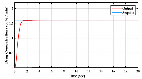
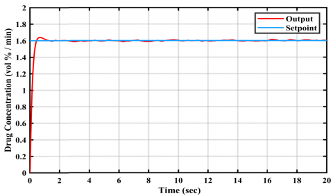
Table 4 depicts the output signal time domain specifications of MPC architectures and the auto-tuned PID. The best MPC results were obtained in the timestep range 0.2 to 0.4 seconds. These results show that the PID controller achieved the lowest rise time, settling time, peak time and minimum settling value. In case of MPC, as the timesteps increased from 0.2 to 0.4 seconds, there was a gradual increase in the rise time and settling time, whereas the peak time recorded a steep rise. Conversely, the minimum/maximum settling values as well as the peak values decreased with increasing timestep durations. However, the overshoot % decreased during timestep increment from 0.2 to 0.35 and again increased at the subsequent 0.4 timestep. Lowest overshoot % was obtained by the 0.35 seconds timestep MPC.
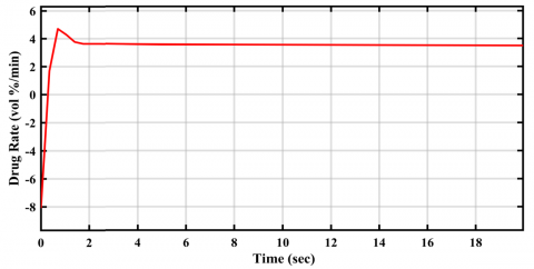
All controllers achieved zero undershoots in output signals. From the perspective of minimum settling time, the PID controller outperformed all explored MPC configurations. However, its response suffered from the highest overshoot % among all. On the other hand, the MPC designed with 0.35 seconds timestep completely eliminated overshoot %. and the elimination of over and undershoots ensures safe and intended drug concentration levels in the patient body, the 0.35 timestep MPC may be preferred for the suggestive anesthetic drug delivery rate application at constant setpoints specified by the anesthesiologists. Figures 5 and 6 show the constant setpoint time domain response plots of the 0.35 seconds timestep MPC output and control signals respectively. Figures 7 and 8 show the corresponding plots for the PID controller. The drug delivery rate suggested by the control signal settling value of the 0.35 timestep MPC is 3.63227% volume per minute. The control signal settling time indicates the time taken by the controller to suggest the optimal anesthetic drug delivery rate to the anesthesiologist, based on the setpoint selected by her/him. In case of constant setpoint, the MPC with 0.35 timestep can provide this suggestive output in just 2 seconds.
Table 4. Output signal time domain specifications of MPC and PID controllers for constant setpoint (1.6)
|
Controller/Parameters |
MPC |
PID |
||||
|
Timestep (s) |
0.2 |
0.25 |
0.3 |
0.35 |
0.4 |
|
|
Rise Time (s) |
0.6013 |
0.6164 |
0.6833 |
0.7252 |
0.7706 |
0.2638 |
|
Settling Time (s) |
1.2616 |
0.9506 |
1.1132 |
1.2419 |
1.368 |
0.8364 |
|
Settling Min (vol %/min) |
1.4512 |
1.4625 |
1.4714 |
1.4502 |
1.457 |
1.4411 |
|
Settling Max (vol %/min) |
1.6345 |
1.62 |
1.5992 |
1.5989 |
1.5985 |
1.6442 |
|
Overshoot (%) |
2.1689 |
1.2701 |
9E-04 |
0 |
7.25E-05 |
2.7961 |
|
Undershoot (%) |
0 |
0 |
0 |
0 |
0 |
0 |
|
Peak (vol %/min) |
1.6345 |
1.62 |
1.5992 |
1.5989 |
1.5985 |
1.6442 |
|
Peak Time (s) |
1.2 |
1.2204 |
19.3283 |
20 |
19.8021 |
0.6544 |
Figure 5. MPC-output signal plot for anesthesia for constant setpoint
Figure 6. MPC-control signal plot for anesthesia for constant setpoint
Figure 7. PID-output signal plot for anesthesia for constant setpoint
Figure 8. PID-control signal plot for anesthesia for constant setpoint
3.3 Constant setpoint with disturbances
This section discusses the control results obtained for cases wherein signal disturbances were considered along with constant setpoint specified by the anesthesiologist.
3.3.1 Disturbance 0.01
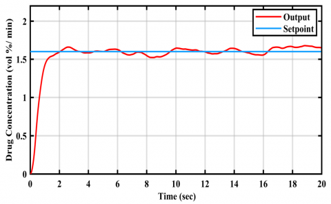
Table 5 depicts the output signal time domain specifications of MPC timestep variations and those of the auto- tuned PID. The best MPC results were obtained in the timestep range 0.5 to 1.75 seconds. These results show that the PID controller achieved the lowest rise time, settling time, peak time and peak/maximum settling value. In case of MPC, as the timesteps increased from 0.5 to 1.75 seconds, there was a gradual increase in settling time. Conversely, the minimum settling value decreased with increasing timestep durations. Rise time, maximum settling value, peak value and peak time increased during timestep increments 0.5 to 1.5, but dropped in the subsequent timestep of 1.75 seconds. Overshoot % did not exhibit any specific trend with increasing timesteps. Lowest overshoot % was obtained by the 1.5 seconds timestep MPC. All controllers achieved zero undershoots in output signals except for the 1.75 seconds timestep MPC. From the perspective of minimum settling time, the PID controller outperformed all explored MPC configurations.
Table 5. Time domain specification of MPC and PID controllers for setpoint 1.6 and noise 0.01
|
Controller/Parameters |
MPC |
PID |
||||
|
Timestep (s) |
0.5 |
0.75 |
5 |
1.5 |
1.75 |
|
|
Rise Time (s) |
1.0851 |
1.4024 |
1.9146 |
2.3165 |
0.5078 |
0.2695 |
|
Settling Time (s) |
16.4783 |
18.9713 |
19.4208 |
18.8438 |
19.2435 |
0.8056 |
|
Settling Min (vol %/min) |
1.5003 |
1.4911 |
1.3494 |
1.1948 |
-0.24 |
1.4472 |
|
Settling Max (vol %/min) |
1.6833 |
1.7194 |
1.819 |
1.8852 |
1.7333 |
1.6398 |
|
Overshoot (%) |
1.3019 |
2.3671 |
3.2504 |
0.0908 |
844.2987 |
2.3114 |
|
Undershoot (%) |
0 |
0 |
0 |
0 |
13.7728 |
0 |
|
Peak (vol %/min) |
1.6833 |
1.7194 |
1.819 |
1.8852 |
1.7333 |
1.6398 |
|
Peak Time (s) |
18.8516 |
18.8 |
18.8 |
19.8499 |
3.7 |
0.7 |
Figure 9. MPC-output signal plot for anesthesia for disturbance 0.01
Figure 10. MPC-control signal plot for anesthesia for disturbance 0.01
Figure 11. PID-output signal plot for anesthesia for disturbance 0.01
Figure 12. PID-control signal plot for anesthesia for disturbance 0.01
However, its response suffered from an overshoot of 2.3114%. On the other hand, the MPC designed with 1.5 seconds timestep minimized overshoot % to 0.0908%. However, its settling time was 18.0382 seconds longer than that of the PID. In fact, settling times of all MPCs were significantly larger than that of PID. This result shows that PID handles noise disturbance much better than MPC with regards to the output settling time for the pharmacokinetic model considered in the present work. However, its overshoot in the concentration of drug absorbed by the body is highly undesirable considering patient safety. On the other hand, the best performing MPC with lowest overshoot (1.5 seconds timestep) took 18 seconds to settle, which is not detrimental since it implies that the patient body would achieve the required drug concentration after 18 seconds of anesthetic drug delivery commencement. Figures 9 and 10 show the constant setpoint/disturbance 0.01 time domain response plots of the 1.5 seconds timestep MPC output and control signals respectively.
Figures 11 and 12 show the corresponding plots for the PID controller. Although the control signal of this MPC did not settle properly, an average of its settling value (after rise time) could be considered as an effective drug delivery rate suggestion to the anesthesiologist. This average settling value for the said MPC is 3.52033, which is quite close to the drug delivery rate suggested by MPC for the same setpoint without any disturbance (3.63227% volume per minute). The control signal settling time, which indicates the time taken by the controller to suggest the optimal anesthetic drug delivery rate to the anesthesiologist, should be at least 10 seconds for the MPC with 1.5 timestep to deliver a reasonable average suggestive value.
3.3.2 Disturbance 0.001
Table 6 depicts the output signal time domain specifications of MPC timestep variations and those of the autotuned PID. The best MPC results were obtained in the timestep range 0.2 to 0.4 seconds. These results shows that the PID controller achieved the lowest rise time, settling time, peak time, and minimum settling value. In case of MPC, as the timesteps increased from 0.2 to 0.4 seconds, there was an increase in rise time, settling time and peak time. Conversely, the minimum/maximum settling and peak values firstly decreased with increasing timestep duration 0.2 to 0.3, and then started increasing at further timestep increments. Overshoot % did not exhibit any specific trend with increasing timesteps. Lowest overshoot % was obtained by the 0.4 seconds timestep MPC.
Table 6. Time domain specification of MPC and PID controllers for setpoint 1.6 and noise 0.001
|
Controller/Parameters |
MPC |
PID |
||||
|
Timestep (s) |
0.2 |
0.25 |
0.3 |
0.35 |
0.4 |
|
|
Rise Time (s) |
0.6185 |
0.6566 |
0.7083 |
0.7583 |
0.8107 |
0.2658 |
|
Settling Time (s) |
8.5832 |
8.5963 |
9.0728 |
9.1532 |
9.2201 |
0.8287 |
|
Settling Min (vol %/min) |
1.4643 |
1.4627 |
1.4563 |
1.4821 |
1.4606 |
1.4523 |
|
Settling Max (vol %/min) |
1.6271 |
1.6221 |
1.6228 |
1.6233 |
1.6239 |
1.6416 |
|
Overshoot (%) |
0.8605 |
0.5341 |
0.5248 |
0.5254 |
0.5232 |
2.5665 |
|
Undershoot (%) |
0 |
0 |
0 |
0 |
0 |
0 |
|
Peak (vol %/min) |
1.6271 |
1.6221 |
1.6228 |
1.6233 |
1.6239 |
1.6416 |
|
Peak Time (s) |
1.1676 |
18.85 |
18.8511 |
18.5 |
18.852 |
0.6501 |
All controllers achieved zero undershoots in output signals. From the perspective of minimum settling time, the PID controller outperformed all explored MPC configurations. However, its response suffered from the highest overshoot (2.5665%) among all explored controllers. On the other hand, the MPC designed with 0.4 seconds timestep minimized overshoot to 0.5232%. However, its settling time was 8.3914 seconds longer than that of the PID. In fact, settling times of all MPCs were significantly larger than that of PID. This result again shows that PID handles noise disturbance much better than MPC with regards to the output settling time for the pharmacokinetic model considered in the present work. However, its overshoot in the concentration of drug absorbed by the body is highly undesirable considering patient safety. On the other hand, the best performing MPC with lowest overshoot (0.4 seconds timestep) took more than 9 seconds to settle, which is not detrimental since it implies that the patient body would achieve the required drug concentration after just 9 seconds of anesthetic drug delivery commencement. Figures 13 and 14 show the constant setpoint/disturbance 0.001-time domain response plots of the 0.4 seconds timestep MPC output and control signals respectively.
Figure 13. MPC-output signal plot for anesthesia for disturbance 0.001
Figure 14. MPC-control signal plot for anesthesia for disturbance 0.001
Figures 15 and 16 show the corresponding plots for the PID controller. Although the control signal of this MPC did not settle properly, an average of its settling value (after rise time) could be considered as an effective drug delivery rate suggestion to the anesthesiologist. This average settling value for the said MPC is 3.57572, which is quite close to the drug delivery rate suggested by MPC for the same setpoint without any disturbance (3.63227% volume per minute). The control signal settling time, which indicates the time taken by the controller to suggest the optimal anesthetic drug delivery rate to the anesthesiologist, should be at least 5 seconds for the MPC with 0.4 seconds timestep to deliver a reasonable average suggestive value.
Figure 15. PID-output signal plot for anesthesia for disturbance 0.001
Figure 16. PID-control signal plot for anesthesia for disturbance 0.001
3.4 Varying setpoint
This section discusses the control results obtained for cases wherein rapid setpoint changes made by the anesthesiologist were considered.
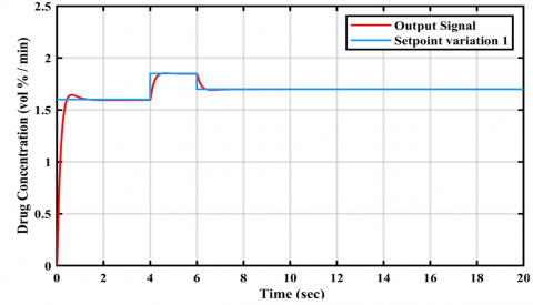
3.4.1 Setpoint variation 1
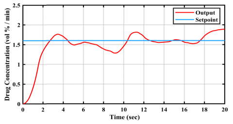
The first setpoint variation included 1.6 (0 to 4 seconds), 1.85 (4 to 6 seconds) and 1.7 (6 to 20 seconds). Table 7 depicts the output signal time domain specifications of MPC architectures and the auto-tuned PID. The best MPC results were obtained in the timestep range 0.25 to 1.5 seconds. These results show that the PID controller achieved the lowest rise time, settling time and peak time. In case of MPC, as the timesteps increased from 0.2 to 1.5 seconds, there was a gradual increase in the rise time, settling time and peak time. Conversely, the maximum settling values, peak values and overshoot % decreased with increasing timestep durations. However, the minimum settling time increased during timestep increment from 0.25 to 0.5 and then increased during the following timestep increments. Lowest overshoot % was obtained by the 1.5 seconds timestep MPC.
Table 7. Time domain specification of MPC and PID controllers for setpoint variation 1
|
Controller/Parameters |
MPC |
PID |
||||
|
Timestep (s) |
0.25 |
0.5 |
0.75 |
1.25 |
1.5 |
|
|
Rise Time (s) |
0.7451 |
1.0721 |
1.3161 |
1.6054 |
1.724 |
0.3236 |
|
Settling Time (s) |
6.6425 |
6.8091 |
6.9757 |
7.6078 |
13.9241 |
6.2038 |
|
Settling Min (vol %/min) |
1.5465 |
1.5502 |
1.5369 |
1.5225 |
1.4173 |
1.5421 |
|
Settling Max (vol %/min) |
1.8507 |
1.8431 |
1.829 |
1.8012 |
1.7895 |
1.8531 |
|
Overshoot (%) |
8.8996 |
8.569 |
7.8803 |
6.5374 |
6.0316 |
9.0439 |
|
Undershoot (%) |
0 |
0 |
0 |
0 |
0 |
0 |
|
Peak (vol %/min) |
1.8507 |
1.8431 |
1.829 |
1.8012 |
1.7895 |
1.8531 |
|
Peak Time (s) |
5.25 |
6 |
6.0625 |
6.7142 |
6.3905 |
4.6129 |
All controllers achieved zero undershoots in output signals. From the perspective of minimum settling time, the PID controller outperformed all explored MPC configurations. However, its response suffered from the highest overshoot % among all. On the other hand, the MPC designed with 1.5 seconds timestep minimized overshoot to 6.0316%. However, its settling time was 7.7203 seconds longer than that of the PID. In fact, settling times of all MPCs were larger than that of PID. This result shows that PID handles the above mentioned setpoint variation much better than MPC with regards to the output settling time for the pharmacokinetic model considered in the present work. However, the overshoots of all controllers in the concentration of drug absorbed by the body are highly undesirable considering patient safety. On the other hand, the best performing MPC with lowest overshoot (1.5 seconds timestep) took more than 13 seconds to settle, which is not detrimental since it implies that the patient body would achieve the required drug concentration after just 13 seconds of anesthetic drug delivery commencement. However, the MPC architectures could not minimise overshoot % as well as they did in the above discussed cases of constant setpoint with and without disturbances. This result shows that extremely quick changes in setpoint selections would result in unavoidable spikes in the resultant drug concentration in the patient body, if the anesthesiologist changes the corresponding drug delivery rates at the short intervals.
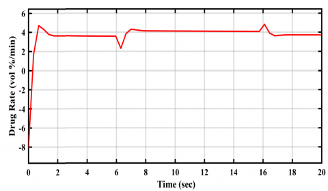
In such cases, the concerned anesthesiologist should wait for the final drug delivery suggestion by the controller based on her/his final setpoint selection before beginning actual drug administration to the patient. Figures 17 and 18 show the time domain response plots of the 1.5 seconds timestep-MPC output and control signals respectively. Figures 19 and 20 show the corresponding plots for the PID controller. Although the control signal of this MPC did not settle properly, the individual averages of its settling values (after rise time) in the respective time periods of the three setpoints could be considered as effective drug delivery rate suggestions to the anesthesiologist. These average settling values for the said MPC were 3.54975, 3.70691 and 3.51985 (% volume per minute). The control signal settling times for the MPC (with 1.5 seconds timestep), which indicate the time taken by the controller to suggest the optimal anesthetic drug delivery rates to the anesthesiologist, would be 4, 6 and 20 seconds for the three setpoints consecutively.
Figure 17. MPC-output signal plot for anesthesia for setpoint variation-1
Figure 18. MPC-control signal plot for anesthesia for setpoint variation-1
Figure 19. PID-output signal plot for anesthesia for setpoint variation-1
Figure 20. PID-control signal plot for anesthesia for setpoint variation-1
3.4.2 Setpoint variation 2
The second setpoint variation included 1.6 (0 to 6 seconds), 1.85 (6 to 16 seconds) and 1.7 (16 to 20 seconds). Table 8 depicts the output signal time domain specifications of MPC architectures and the auto-tuned PID. The best MPC results were obtained in the timestep range 0.20 to 0.4 seconds. These results show that the PID controller achieved the lowest rise time, settling time and peak time. In case of MPC, as the timesteps increased from 0.2 to 0.4 seconds, there was a gradual increase in the rise time. Conversely, the maximum/minimum settling values and peak values decreased with increasing timestep durations. However, the settling time increased during timestep increment from 0.2 to 0.35 seconds and then decreased during the following timestep increment. Overshoot % followed the exactly opposite trend as that of settling time. Lowest overshoot % was obtained by the 0.35 seconds timestep MPC.
Table 8. Time domain specification of MPC and PID controllers for setpoint variation 2
|
Controller/Parameters |
MPC |
PID |
||||
|
Timestep (s) |
0.2 |
0.25 |
0.3 |
0.35 |
0.4 |
|
|
Rise Time (s) |
0.6876 |
0.7454 |
0.82 |
0.893 |
0.9554 |
0.3238 |
|
Settling Time (s) |
16.6279 |
16.65 |
16.8777 |
16.8145 |
16.7611 |
16.2301 |
|
Settling Min (vol %/min) |
1.5316 |
1.5465 |
1.5397 |
1.5349 |
1.5385 |
1.5421 |
|
Settling Max (vol %/min) |
1.8545 |
1.8509 |
1.849 |
1.8486 |
1.8481 |
1.855 |
|
Overshoot (%) |
9.0739 |
8.845 |
8.7991 |
8.7834 |
8.805 |
9.1279 |
|
Undershoot (%) |
0 |
0 |
0 |
0 |
0 |
0 |
|
Peak (vol %/min) |
1.8545 |
1.8509 |
1.849 |
1.8486 |
1.8481 |
1.855 |
|
Peak Time (s) |
7.2 |
7.25 |
16.2 |
16.1 |
15.98 |
6.6367 |
All controllers achieved zero undershoots in output signals. From the perspective of minimum settling time, the PID controller outperformed all explored MPC configurations. However, its response suffered from the highest overshoot % among all. On the other hand, the MPC designed with 0.35 seconds timestep minimized overshoot to 8.7834%. Its settling time was just 0.5844 seconds longer than that of the PID. In fact, settling times of all MPCs were minimally larger than that of PID. This result shows that PID handled the above mentioned setpoint variation only marginally better than MPC with regards to the output settling time for the pharmacokinetic model considered in the present work. However, overshoots of all controllers in the concentration of drug absorbed by the body are highly undesirable considering patient safety. On the other hand, the best performing MPC with lowest overshoot (0.35 seconds timestep) took more than 16 seconds to settle, which is not detrimental since it implies that the patient body would achieve the required drug concentration after only 16 seconds of anesthetic drug delivery commencement. However, the MPC architectures could not minimize overshoot % as well as they did in the above discussed cases of constant setpoint with and without disturbances. This result shows that extremely quick changes in setpoint selections would result in unavoidable spikes in the resultant drug concentration in the patient body, if the anesthesiologist changes the corresponding drug delivery rates at short intervals. In such cases, the concerned anesthesiologist should wait for the final drug delivery suggestion by the controller based on her/his final setpoint selection before beginning actual drug administration to the patient. Figures 21 and 22 show the time domain response plots of the 0.35 seconds timestep MPC output and control signals respectively. Figures 23 and 24 show the corresponding plots for the PID controller. Although the control signal of this MPC did not settle properly, the individual averages of its settling values (after rise time) in the respective time periods of the three setpoints could be considered as effective drug delivery rate suggestions to the anesthesiologist. These average settling values for the said MPC were 3.72556, 4.04702 and 3.71857 (% volume per minute). The control signal settling times for the MPC (with 1.5 seconds timestep), which indicate the time taken by the controller to suggest the optimal anesthetic drug delivery rates to the anesthesiologist, would be 6, 16 and 20 seconds for the three setpoints consecutively.
Figure 21. MPC-output signal plot for anesthesia for setpoint variation-2
Figure 22. MPC-control signal plot for anesthesia for setpoint variation-2
Figure 23. PID-output signal plot for anesthesia for setpoint variation-2
Figure 24. PID-control signal plot for anesthesia for setpoint variation-2
Table 9. Time domain specification of MPC and PID controllers for setpoint variation 3
|
Controller/Parameters |
MPC |
PID |
||||
|
Timestep (s) |
0.25 |
0.5 |
0.75 |
0.1 |
1.25 |
|
|
Rise Time (s) |
0.7451 |
1.0719 |
1.3161 |
1.4804 |
1.6089 |
0.3236 |
|
Settling Time (s) |
3.6444 |
3.7658 |
3.8843 |
4.0992 |
5.0921 |
3.1991 |
|
Settling Min (vol %/min) |
1.5465 |
1.5502 |
1.5369 |
1.5285 |
1.5249 |
1.5421 |
|
Settling Max (vol %/min) |
1.8434 |
1.814 |
1.7729 |
1.7824 |
1.7947 |
1.8503 |
|
Overshoot (%) |
8.465 |
6.8553 |
4.5761 |
5.2882 |
6.1451 |
8.879 |
|
Undershoot (%) |
0 |
0 |
0 |
0 |
0 |
0 |
|
Peak (vol %/min) |
1.8434 |
1.814 |
1.7729 |
1.7824 |
1.7947 |
1.8503 |
|
Peak Time (s) |
3.0299 |
3.1226 |
3.4042 |
3.4409 |
4.2132 |
2.6417 |
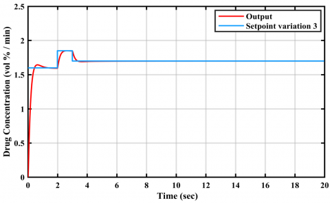
3.4.3 Setpoint variation 3
The third setpoint variation included 1.6 (0 to 2 seconds), 1.85 (2 to 3 seconds) and 1.7 (3 to 20 seconds). Table 9 depicts the output signal time domain specifications of MPC architectures and the auto-tuned PID. The best MPC results were obtained in the timestep range 0.25 to 1.25 seconds. These results show that the PID controller achieved the lowest rise time, settling time and peak time. In case of MPC, as the timesteps increased from 0.25 to 1.25 seconds, there was a gradual increase in the rise time, settling time and peak time. The minimum settling values increased during timestep increment from 0.25 to 0.5 seconds and then decreased during the following timestep increments. Conversely, max settling/peak values and overshoot % initially decreased during timestep increment from 0.25 to 0.75 seconds and then increased during the subsequent timestep increments. Lowest overshoot % was obtained by the 0.75 seconds timestep MPC.
Figure 25. MPC-output signal plot for anesthesia for constant setpoint-new mammalian rate constant
Figure 26. PID-output signal plot for anesthesia for constant setpoint-new mammalian rate constant
3.5 New mammalian rate constant
The MPC and PID controllers were employed with updated mammalian rate constants utilizing the isodamping approach. The settling time results were 3.46901 seconds for PID and 10.6297 seconds for MPC, while the overshoot percentages were 11.89% for PID and 10.2% for MPC.
While PID exhibited superior performance in settling time compared to MPC, MPC showed lower overshoot levels compared to PID which is shown in Figures 25 and 26.
The performance criteria such as integral square error as one of the performance index was calculated. The effectiveness and robustness of PID and MPC control strategies under different conditions, 1. Effectiveness: PID Control: Generally, lower ISE values indicate better control performance. From the Table 10, PID control demonstrates effectiveness in maintaining low ISE values across various conditions. For instance, under constant setpoint conditions, the ISE values for PID control range from 101.42 to 1345.60, which suggests consistent performance in minimizing error. MPC Control: MPC control also shows effectiveness in controlling the system, as indicated by generally low ISE values. However, in some cases, such as under constant setpoint with disturbance conditions, MPC performs less effectively compared to PID. For instance, under disturbance of 0.01, MPC has higher ISE values compared to PID (1764.30 vs. 111.38).
Table 10. Integral square error (ISE) of MPC and PID
|
Control Conditions |
ISE |
|
|
PID |
MPC |
|
|
Constant setpoint |
1345.60 |
1532.30 |
|
Constant setpoint with disturbance 0.01 |
111.38 |
1764.30 |
|
Constant setpoint with disturbance 0.001 |
101.42 |
407.90 |
|
Setpoint variation 1 |
34.81 |
298.85 |
|
Setpoint variation 2 |
35.73 |
226.17 |
|
Setpoint variation 3 |
32.86 |
199.91 |
PID control demonstrates robustness under different conditions, maintaining relatively consistent performance across all scenarios. While the ISE values may vary depending on the condition, they generally remain within a certain range, indicating stability and robustness of the PID control strategy. MPC Control: MPC control shows varying degrees of robustness under different conditions. While it performs well under some conditions (e.g., setpoint variation 3 with an ISE of 199.91), it shows higher sensitivity to disturbances compared to PID control. This suggests that MPC may require additional tuning or adaptation to maintain robust performance in the presence of disturbances.
Overall, while both PID and MPC control strategies demonstrate effectiveness in controlling the system, PID control appears to be more robust across different conditions, with generally lower ISE values and less sensitivity to disturbances. However, MPC control may offer advantages in certain scenarios, particularly in cases where predictive control or handling of complex dynamics is required.
All controllers achieved zero undershoots in output signals. From the perspective of minimum settling time, the PID controller outperformed all explored MPC configurations. However, its response suffered from the highest overshoot % among all. On the other hand, the MPC designed with 0.75 seconds timestep minimized overshoot to 4.5761%. Its settling time was just 0.6852 seconds longer than that of the PID. In fact, settling times of all MPCs were marginally larger than that of the PID. This result shows that PID handled the above mentioned setpoint variation only marginally better than MPC with regards to the output settling time for the pharmacokinetic model considered in the present work. However, overshoots of all controllers in the concentration of drug absorbed by the body are highly undesirable considering patient safety.
Figure 27. MPC-output signal plot for anesthesia for setpoint variation-3
Figure 28. MPC-control signal plot for anesthesia for setpoint variation-3
The best performing MPC with lowest overshoot (0.75 seconds timestep) took more than 3 seconds to settle, which is not detrimental since it implies that the patient body would achieve the required drug concentration after only 3 seconds of anesthetic drug delivery commencement. However, the MPC architectures could not minimize overshoot % as well as they did in the previously discussed cases of constant setpoint with and without disturbances. This result also shows that extremely quick changes in setpoint selections would result in unavoidable spikes in the resultant drug concentration in the patient body, if the anesthesiologist changes the corresponding drug delivery rates at short intervals. In such cases, the concerned anesthesiologist should wait for the final drug delivery suggestion by the controller based on her/his final setpoint selection before beginning actual drug administration to the patient. Figures 27 and 28 show the time domain response plots of the 0.75 seconds timestep MPC output and control signals respectively. Figures 29 and 30 show the corresponding plots for the PID controller. Although the control signal of this MPC did not settle properly, the individual averages of its settling values (after rise time) in the respective time periods of the three setpoints could be considered as effective drug delivery rate suggestions to the anesthesiologist. These average settling values for the said MPC were 3.50841, 3.80399 and 3.755623 (% volume per minute). The control signal settling times for the MPC (with 1.5 seconds timestep), which indicate the time taken by the controller to suggest the optimal anesthetic drug delivery rates to the anesthesiologist, would be 2, 3 and 20 seconds for the three setpoints consecutively.
Figure 29. PID-output signal plot for anesthesia for setpoint variation-3
Figure 30. PID-control signal plot for anesthesia for setpoint variation-3
This study proposed a model predictive control (MPC) based methodology to suggest the optimal anesthetic drug delivery rate to an anesthesiologist based on the required drug concentration level in the patient body for achieving adequate sedation during surgery. The MPC controller was designed on a pharmacokinetics model that accounted for the inhaled drug transmission rates between the lungs and four other primary tissue groups in the human body as well as the drug exhalation/excretion rate from the body. The MPC controllers were tuned for minimal over and undershoots in output signal responses (drug concentration in body) across varying conditions such as constant setpoint, setpoint with disturbances (0.1 and 0.01) and setpoint variations (three variation designs having three setpoint steps each).
The MPC control results were compared to those of an auto tuned PID controller for the same conditions. Macro results showed that: firstly, all explored controllers successfully eliminated output signal undershoots. Secondly, the auto tuned PID controller minimized output settling time in all cases. Thirdly, the MPC architectures minimized output overshoots in all cases. Considering the possible severity of output overshoot implications in terms of anesthetic overdosage in patient body, the explored MPC architectures present safer alternatives to PID for the suggestive drug delivery rate application. Moreover, the MPC with the maximum delayed settling time took about 18 seconds to settle, which is not at all detrimental since it implies that the patient body would achieve the required drug concentration after just 18 seconds of anesthetic drug delivery commencement. Considering the control signal results, the best MPC would be able to suggest the optimum drug delivery rate to the anesthesiologist within 2 seconds in case of constant setpoint. The same would be suggested by the respective best performing MPC after 5 and 10 seconds for the constant setpoint with 0.001 and 0.01 disturbances respectively. In setpoint variation cases, the respective best performing MPC can suggest drug delivery rate immediately after the setpoint is changed, or at least ten seconds after the final setpoint selection. The application of a model predictive control (MPC) system to manage anesthetic drug delivery has promising advantages and difficulties. This system is intended to improve the situation for the patient by reducing overshoot with respect to drug concentrations in the patient’s bloodstream and thus the risk of an overdose. Also, it can reduce the burden on anesthesiologists in helping the clinical decision-making process on drug dosing so that they can dedicate time and effort to other essential patient care related activities. However, there is a need for precautions when translating simulation results for their applicability in the real world. Models, no matter how realistic, do not recreate the real-life conditions of surgeries and patients, or some unpredictable and unforeseen circumstances. Possible risks are technical problems, reactions of patients towards the robots and interfacing issues with currently used equipment. The anesthesiologist’s function continues to be important, assuming responsibility for supervising the system, verifying its recommendations and manually correcting the system if needed.
The future scope of this study may include further exploration of MPC architectures to achieve better control results. Moreover, actual patients’ data may be used for system identification of the pharmacokinetics- pharmacodynamics based anesthesia system followed by its control. Also, conducting clinical trials, refining the pharmacokinetics model, robustness testing, and evaluating the system’s usability.
[1] Zurn, P., Dal Poz, M.R., Stilwell, B., Adams, O. (2004). Imbalance in the health workforce. Human Resources for Health, 2: 1-12. https://doi.org/10.1186/1478-4491-2-13
[2] Lopes, M.A., Almeida, A.S., Almada-Lobo, B. (2015). Handling healthcare workforce planning with care: Where do we stand? Human Resources for Health, 13: 1-19. https://doi.org/10.1186/s12960-015-0028-0
[3] Pannocchia, G., Laurino, M., Landi, A. (2010). A model predictive control strategy toward optimal structured treatment interruptions in anti-HIV therapy. IEEE Transactions on Biomedical Engineering, 57(5): 1040-1050. http://doi.org/10.1109/TBME.2009.2039571
[4] Shah, P., Sekhar, R. (2019). Closed loop system identification of a DC motor using fractional order model. In 2019 International Conference on Mechatronics, Robotics and Systems Engineering (MoRSE), pp. 69-74. https://doi.org/10.1109/MoRSE48060.2019.8998744
[5] Sekhar, R., Singh, T., Shah, P. (2019). ARX/ARMAX modeling and fractional order control of surface roughness in turning nano-composites. In 2019 International Conference on Mechatronics, Robotics and Systems Engineering (MoRSE), pp. 97-102. https://doi.org/10.1109/MoRSE48060.2019.8998654
[6] Gao, J., Gu, H., Yang, Y.W., Yuan, P., Poloei, H. (2022). Improve microbial fuel cell efficiency using receding horizon predictive control. Journal of New Materials for Electrochemical Systems, 25(1): 72-78. https://doi.org/10.14447/jnmes.v25i1.a10
[7] Khather, S.I., Ibrahim, M.A., Abdullah, A.I. (2023). Review and performance analysis of nonlinear model predictive control—current prospects, challenges and future directions. Journal Européen des Systèmes Automatisés, 56(4): 593-603. https://doi.org/10.18280/jesa.560409
[8] Azar, A.T. (2020). Control Applications for Biomedical Engineering Systems. Academic Press.
[9] Pawłowski, A., Schiavo, M., Latronico, N., Paltenghi, M., Visioli, A. (2024). Drug co‐administration in anesthesia using event‐based MPC. International Journal of Robust and Nonlinear Control. https://doi.org/10.1002/rnc.7080
[10] Milanesi, M., Consolini, L., Di Credico, G., Latronico, N., Laurini, M., Paltenghi, M., Schiavo, M., Visioli, A. (2024). Human-imitating control of depth of hypnosis combining MPC and event-based PID strategies. IEEE Control Systems Letters, 8: 580-585. https://doi.org/10.1109/LCSYS.2024.3399093
[11] Dhandore, A., Mhatre, P., Bhole, K. (2022). Prediction of drug events using machine learning. In the 2022 4th International Conference on Advances in Computing, Communication Control and Networking (ICAC3N), Greater Noida, India, pp. 577-582. https://doi.org/10.1109/ICAC3N56670.2022.10074327
[12] Pannocchia, G., Rawlings, J.B. (2003). Disturbance models for offset-free model-predictive control. AIChE Journal, 49(2): 426-437. https://doi.org/10.1002/aic.690490213
[13] Krishna, P.S., Rao, P.G.K. (2024). Fractional-order PID controller for blood pressure regulation using genetic algorithm. Biomedical Signal Processing and Control, 88: 105564. https://doi.org/10.1016/j.bspc.2023.105564
[14] Medvedev, A., Zhusubaliyev, Z.T., Rosén, O., Silva, M.M. (2019). Oscillations-free PID control of anesthetic drug delivery in neuromuscular blockade. Computer Methods and Programs in Biomedicine, 171: 119-131. https://doi.org/10.1016/j.cmpb.2016.07.025
[15] Hosseinzadeh, M. (2020). Robust control applications in biomedical engineering: Control of depth of hypnosis. In Control Applications for Biomedical Engineering Systems, pp. 89-125. https://doi.org/10.1016/B978-0-12-817461-6.00004-4
[16] Ramesh, N.H.A.R., Ghazali, M.R., Ahmad, M.A. (2021). Sigmoid PID based adaptive safe experimentation dynamics algorithm of portable Duodopa pump for Parkinson’s disease patients. Bulletin of Electrical Engineering and Informatics, 10(2): 632-639. https://doi.org/10.11591/eei.v10i2.2542
[17] Sekhar, R., Singh, T.P., Shah, P. (2022). Machine learning based predictive modeling and control of surface roughness generation while machining micro boron carbide and carbon nanotube particle reinforced Al-Mg matrix composites. Particulate Science and Technology, 40(3): 355-372. https://doi.org/10.1080/02726351.2021.1933282
[18] Garcia, C.E., Prett, D.M., Morari, M. (1989). Model predictive control: Theory and practice—A survey. Automatica, 25(3): 335-348. https://doi.org/10.1016/0005-1098(89)90002-2
[19] De Keyser, R.M., Van de Velde, P.G., Dumortier, F. (1988). A comparative study of self-adaptive long-range predictive control methods. Automatica, 24(2): 149-163. https://doi.org/10.1016/0005-1098(88)90024-6
[20] Scattolini, R., Bittanti, S. (1990). On the choice of the horizon in long-range predictive control—Some simple criteria. Automatica, 26(5): 915-917. https://doi.org/10.1016/0005-1098(90)90009-7
[21] Clarke, D., Scattolini, R. (1991). Constrained receding-horizon predictive control. IEE Proceedings D (Control Theory and Applications), 138(4): 347-354. https://doi.org/10.1049/ip-d.1991.0047
[22] Qin, S.J., Badgwell, T.A. (2003). A survey of industrial model predictive control technology. Control Engineering Practice, 11(7): 733-764. https://doi.org/10.1016/S0967-0661(02)00186-7
[23] Jalali, A.A., Nadimi, V. (2006). A survey on robust model predictive control from 1999-2006. In 2006 International Conference on Computational Intelligence for Modelling Control and Automation and International Conference on Intelligent Agents Web Technologies and International Commerce (CIMCA’06), pp. 207-207. https://doi.org/10.1109/CIMCA.2006.29
[24] Warren, A.L., Marlin, T.E. (2004). Constrained MPC under closed-loop uncertainty. In Proceedings of the 2004 American Control Conference, pp. 4607-4612. https://doi.org/10.23919/ACC.2004.1384037
[25] Abu-Ayyad, M., Dubay, R. (2007). Real-time comparison of a number of predictive controllers. ISA Transactions, 46(3): 411-418. https://doi.org/10.1016/j.isatra.2007.02.005
[26] Mesbah, A. (2016). Stochastic model predictive control: An overview and perspectives for future research. IEEE Control Systems Magazine, 36(6): 30-44. https://doi.org/10.1109/MCS.2016.2602087
[27] Orukpe, P. (2012). Model predictive control fundamentals. Nigerian Journal of Technology, 31(2): 139-148. https://doi.org/10.1007/978-3-030-24570-2_2
[28] Al-Gherwi, W., Budman, H., Elkamel, A. (2013). A robust distributed model predictive control based on a dual-mode approach. Computers & Chemical Engineering, 50: 130-138. https://doi.org/10.1016/j.compchemeng.2012.11.002
[29] Allgöwer, F., Zheng, A. (2012). Nonlinear Model Predictive Control. Birkhäuser.
[30] Findeisen, R., Allgöwer, F., Biegler, L.T. (2007). Assessment and Future Directions of Nonlinear Model Predictive Control. Springer. https://doi.org/10.1007/978-3-540-72699-9
[31] Knyazev, A., Malyshev, A. (2016). Sparse preconditioning for model predictive control. In 2016 American Control Conference (ACC), pp. 4494-4499. https://doi.org/10.1109/ACC.2016.7526060
[32] Bemporad, A., Morari, M., Dua, V., Pistikopoulos, E.N. (2002). The explicit linear quadratic regulator for constrained systems. Automatica, 38(1): 3-20. https://doi.org/10.1016/S0005-1098(01)00174-1
[33] Ammirati, E., Wang, D.W. (2020). SARS-CoV-2 inflames the heart. The importance of awareness of myocardial injury in COVID-19 patients. International Journal of Cardiology, 311: 122. https://doi.org/10.1016%2Fj.ijcard.2020.03.086
[34] Savoca, A., Barazzetta, J., Pesenti, G., Manca, D. (2018). Model predictive control for automated anesthesia. Computer Aided Chemical Engineering, 43: 1631-1636. https://doi.org/10.1016/B978-0-444-64235-6.50284-9
[35] Ingole, D.D., Sonawane, D.N., Naik, V.V., Ginoya, D.L., Patki, V.V. (2013). Linear model predictive controller for closed-loop control of intravenous anesthesia with time delay. International Journal on Control System and Instrumentation, 4(1): 8. https://doi.org/01.IJCSI.4.1.1063
[36] Sawaguchi, Y., Furutani, E., Shirakami, G., Araki, M., Fukuda, K. (2008). A model-predictive hypnosis control system under total intravenous anesthesia. IEEE Transactions on Biomedical Engineering, 55(3): 874-887. https://doi.org/10.1109/TBME.2008.915670
[37] Ghita, M., Neckebroek, M., Muresan, C., Copot, D. (2020). Closed-loop control of anesthesia: Survey on actual trends, challenges and perspectives. IEEE Access, 8: 206264-206279. https://doi.org/10.1109/ACCESS.2020.3037725
[38] Ilyas, M., Khaqan, A., Iqbal, J., Riaz, R.A. (2017). Regulation of hypnosis in propofol anesthesia administration based on non-linear control strategy. Revista Brasileira de Anestesiologia, 67: 122-130. https://doi.org/10.1016/j.bjane.2015.08.011
[39] van Heusden, K., Ansermino, J.M., Soltesz, K., Khosravi, S., West, N., Dumont, G.A. (2013). Quantification of the variability in response to propofol administration in children. IEEE Transactions on Biomedical Engineering, 60(9): 2521-2529. https://doi.org/10.1109/TBME.2013.2259592
[40] Coppens, M.J., Eleveld, D.J., Proost, J.H., Marks, L.A., Van Bocxlaer, J.F., Vereecke, H., Struys, M.M. (2011). An evaluation of using population pharmacokinetic models to estimate pharmacodynamic parameters for propofol and bispectral index in children. The Journal of the American Society of Anesthesiologists, 115(1): 83-93. https://doi.org/10.1097/ALN.0b013e31821a8d80
[41] Bibian, S., Ries, C.R., Huzmezan, M., Dumont, G. (2005). Introduction to automated drug delivery in clinical anesthesia. European Journal of Control, 11(6): 535-557. https://doi.org/10.3166/ejc.11.535-557
[42] Yasuda, N., Lockhart, S.H., Eger, E.I., Weiskopf, R.B., Liu, J., Laster, M., Taheri, S., Peterson, N.A. (1991). Comparison of kinetics of sevoflurane and isoflurane in humans. Anesthesia & Analgesia, 72(3): 316-324. http://doi.org/10.1213/00000539-199103000-00007
[43] Gorinevsky. (2005). Lecture notes. https://web.stanford.edu/class/archive/ee/ee392m/ee392m.1056/ Lecture14 MPC.pdf, accessed on 12 Jun. 2020.
[44] MATHWORK. (n.d.). Simulink control design documentation. https://www.mathworks.com/help/slcontrol/, accessed on 12 Jan. 2020.
[45] Pawłowski, A., Schiavo, M., Latronico, N., Paltenghi, M., Visioli, A. (2023). Event-based MPC for propofol administration in anesthesia. Computer Methods and Programs in Biomedicine, 229: 107289. https://doi.org/10.1016/j.cmpb.2022.107289
[46] Delgado-Herrera, L., Ostroff, R.D., Rogers, S.A. (2001). Sevoflurane: Approaching the ideal inhalational anesthetic a pharmacologic, pharmacoeconomic, and clinical review. CNS Drug Reviews, 7(1): 48-120. https://doi.org/10.1111/j.1527-3458.2001.tb00190.x