Pankaj Dumka*![]() | Rishika Chauhan
| Rishika Chauhan![]() | Rohit Mishra
| Rohit Mishra![]() | Darshana Dave
| Darshana Dave![]() | Chandrakant Sonawane
| Chandrakant Sonawane![]() | Anand Pandey
| Anand Pandey![]() | Ghanshyam Tejani
| Ghanshyam Tejani![]()
© 2025 The authors. This article is published by IIETA and is licensed under the CC BY 4.0 license (http://creativecommons.org/licenses/by/4.0/).
OPEN ACCESS
This article explores the application of Monte Carlo simulation to model the two-dimensional Laplace equation which is commonly used in the steady-state heat conduction problems. By using statistical random walk principles, the study develops a Python-based algorithm to approximate solutions for the Laplace equation having fixed boundary (Dirichlet) conditions. The methodology involves formulating probability-based steps, discretizing the equation, and simulating particle paths to estimate temperatures at each grid point. A Python program has been developed to automate this process which has been tested using a sample problem. The results showed excellent agreement with analytical solutions, achieving 98% accuracy with 2000 random walks per node. The findings highlight the trade-off between increased accuracy and computational effort, as accuracy improves with a higher number of random walks. This approach and the provided Python code offer researchers a framework for applying Monte Carlo methods to similar problems and thus illustrate the adaptability of Python for complex simulations.
heat conduction, two-dimensional heat conduction, Monte Carlo simulation, random walk, Python programming, Laplace equation
Often, in many heat transfer studies, steady state solutions are required, and to understand them, the two - dimensional (2D) Laplace equation is solved [1]. Modelling 2D heat conduction is important for understanding steady-state temperature distributions in various engineering applications, such as thermal insulation, electronics cooling, and material processing. Conventional methods, including analytical solutions and deterministic numerical procedures like finite difference or finite element methods, are well-established for solving such problems. However, these approaches often require complex mathematical formulations and boundary condition handling, especially in cases with irregular geometries or variable material properties. Monte Carlo simulations (MC) provide a valuable choice by approaching the problem statistically rather than analytically. This statistical view offers flexibility in handling the diverse boundary conditions and geometries thereby making it particularly useful in applications where deterministic methods may be difficult to implement. Many studies on various facets of 2D heat transport provide both analytical and numerical data [2, 3]. Yet, there is a dearth of literature that not only approaches the heat transfer problem statistically but also explains and illustrates the solution in a way that is simple to reproduce [4]. The MC method for heat conduction relies on simulating random particle movements or "walks" to guess the temperature distribution, making it an intuitive and adaptable approach. This method by-passes the need for detailed analytical formulations by forming probabilistic rules for particle movement, which ultimately approximate the heat conduction process. Regardless of its advantages, MC methods are less frequently applied to heat transfer problems, especially in two-dimensional contexts, due to a lack of straightforward, reproducible implementation workflows. This study addresses this gap by developing a clear, replicable framework for using MC in 2D heat conduction scenarios, explaining its applicability through a practical Python implementation.
Previous studies that have used MC methods in heat transfer which generally focus on complex systems, often at three-dimensional scales, or utilize stochastic approaches within deterministic frameworks to solve specific boundary or material uncertainties. However, literature is sparse on using the MC simulation exclusively for solving the 2D Laplace equation in steady-state heat conduction, mainly with a focus on accessibility for researchers and practitioners who may lack extensive programming or analytical expertise. This paper seeks to address these limitations by creating a simple, replicable model that showcases MC simulation as a primary method for 2D heat conduction, which could be especially valuable for educational and preliminary research purposes. As a result, the authors of this research study felt the necessity to develop a piece that would concentrate on the use of MC simulation in a situation involving 2D heat conduction. This simulation is similar to playing a game [5, 6]. The solution can be found without delving into the problem's analytical nature if the game's rules are established for a certain kind of problem. In order to write the temperature at any node in terms of its surrounding nodes and their respective uncertainties, the differential equations in the heat transfer problem are first discretized, as is done in the finite difference techniques. Random walks are obtained from that node, and they are used to predict the node's temperature. The method's strongest feature is that, with the exception of boundary nodes, it can tell the value at discrete locations without knowing about other points if one has to know the temperature at any particular point [7].
The quantity of randomly generated numbers (random walks) created must be sufficient to ensure the accuracy of the solutions acquired from the MC simulation. Because performing the operation by hand is not an option, computer programmes must be created instead. Python programming is a popular choice for mathematical and scientific computation because of its simple syntax and ease of use [8-15]. Additionally, highly robust and extensive are the libraries for arrays (NumPy) and data visualisation (Matplotlib) [16-20]. In addition to filling this procedural gap, the use of Python for implementing the MC simulation brings several unique benefits. Python is increasingly popular in scientific computing due to its readability, large libraries, and active user community. By using Python’s NumPy for array manipulation and Matplotlib for visualization, this study provides a user-friendly approach that enables readers to quickly adopt and familiarize the code to their own studies. The MC model and code presented in this article offer a starting point for extending the simulations to more complex heat transfer problems, where Python’s abilities can be further exploited to include additional physical factors or boundary conditions.
The differential equations are discretized in this article after a description of the heat conduction problem. Both the implementation process and the MC algorithm are described, together with Python programming. A 2D heat conduction problem is taken to check the Python program.
Ultimately, this study aims to provide a bridge between traditional heat transfer modelling techniques and statistical approaches by illustrating the practicality and effectiveness of MC simulations in solving 2D steady-state conduction problems. By demonstrating that MC simulations can achieve high accuracy (98% agreement with analytical solutions in this case) with an increase in computational resources, this study highlights the potential of MC methods as an efficient and scalable alternative. This approach not only expands the toolkit available to researchers but also offers an accessible framework for solving problems that may be difficult to approach using conventional methods, marking a significant step towards broader adoption of statistical simulation methods in heat transfer analysis.
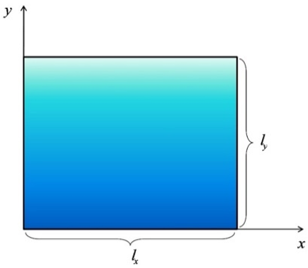
Consider a two-dimensional rectangular domain as shown in Figure 1.
Figure 1. Heat conduction in 1D slab
In this figure, the rectangular domain represents a two-dimensional surface where heat conduction is happening in a steady-state manner. Each boundary of this domain is held at some fixed temperature ($T$), simulating the thermal conditions one might encounter in a heated metal plate or a similar planar material. This arrangement will allow to focus on heat conduction within the boundaries without the need for external influences. The domain length in $x$ and $y$ directions are ${{\ell }_{x}}$ and ${{\ell }_{y}}$ respectively, and it has been assumed that the temperature variation occurs only within this plane (i.e., there is no variation normal to the plane). This assumption is often valid for thin plates where the thickness of the plate is small compared to the other dimensions. The boundary temperatures of the domain are specified. The domain length in $x$ and $y$ directions are ${{\ell }_{x}}$ and ${{\ell }_{y}}$ respectively. As there is no variation in the temperature in the directions normal to the plane of paper, the problem comes under the category of 2D conduction.
The choice of the rectangular domain is both practical and analytically suitable, as it aligns with commonly faced shapes in engineering and materials science, such as plates, walls, and panels. The rectangular geometry allows for direct application of the finite difference method on a uniform grid, enabling a systematic exploration of 2D heat conduction performance. However, the principles and approach used here can be extended to other geometries, such as circular or irregular domains. However, these would require modified discretization schemes and possibly different boundary conditions to address their unique shapes.
The governing equation for 2D steady state heat conduction is Laplace equation which is shown in Eq. (1).
${{\nabla }^{2}}T=\frac{{{\partial }^{2}}T}{\partial {{x}^{2}}}+\frac{{{\partial }^{2}}T}{\partial {{y}^{2}}}=0$ (1)
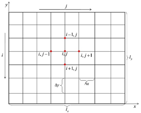
Now discretizing the Eq. (1) in the domain using a second order finite difference scheme with the help of the grid shown in Figure 2 will result in Eq. (2).
Figure 2. Computational grid
$\frac{{{T}_{i,j+1}}-2{{T}_{i,j}}+{{T}_{i,j-1}}}{\text{ }\!\!\Delta\!\!\text{ }{{x}^{2}}}+~\frac{{{T}_{i+1,j}}-2{{T}_{i,j}}+{{T}_{i-1,j}}}{\text{ }\!\!\Delta\!\!\text{ }{{y}^{2}}}=0$ (2)
On further simplification, Eq. (2) becomes:
${{T}_{i}}=\frac{1}{2\left( {{\alpha }^{2}}+1 \right)}{{T}_{i,j+1}}+\frac{1}{2\left( {{\alpha }^{2}}+1 \right)}{{T}_{i,j-1}}+\frac{{{\alpha }^{2}}}{2\left( {{\alpha }^{2}}+1 \right)}{{T}_{i-1,j}}+\frac{{{\alpha }^{2}}}{2\left( {{\alpha }^{2}}+1 \right)}{{T}_{i+1,j}}$ (3)
where, $\alpha =\frac{\text{ }\!\!\Delta\!\!\text{ }x}{\text{ }\!\!\Delta\!\!\text{ }y}$. From the point of view of MC simulation, the coefficients of neighbouring points can be written in terms of probability of random walk in the left, right, top and bottom directions as shown in Eq. (4):
${{T}_{i}}=p_{x}^{+}{{T}_{i,j+1}}+p_{x}^{-}{{T}_{i,j-1}}+p_{y}^{+}{{T}_{i+1,j}}+p_{y}^{-}{{T}_{i-1,j}}$ (4)
where,
$p_{x}^{+}=\frac{1}{2\left( {{\alpha }^{2}}+1 \right)}$; $p_{x}^{-}=\frac{1}{2\left( {{\alpha }^{2}}+1 \right)}$; $p_{y}^{+}=\frac{{{\alpha }^{2}}}{2\left( {{\alpha }^{2}}+1 \right)}$; $p_{y}^{-}=\frac{{{\alpha }^{2}}}{2\left( {{\alpha }^{2}}+1 \right)}$.
The probabilities $p_{x}^{+}$, $p_{x}^{-}$, $p_{y}^{+}$, and $p_{y}^{-}$ show the likelihood of the temperature at point $(i, j)$ being influenced by its neighbouring points in the positive and negative $x$ and $y$ directions. These probabilities are developed from the coefficients in the discretized finite difference equation, and they ensure that the influence of each neighbouring temperature is appropriately weighted in the random walk process. For example, $p_{x}^{+}$ and $p_{x}^{-}$ determine the chances of moving to the right or left (in the $x$ direction), while $p_{y}^{+}$ and $p_{y}^{-}$ correspond to the upward and downward movement (in the $y$ direction). The sum of these probabilities is unity, thereby ensuring that every step in the random walk conforms to a balanced distribution over all the possible directions.
For the sake of simplicity, if one considers $\text{ }\!\!\Delta\!\!\text{ }x=\text{ }\!\!\Delta\!\!\text{ }y$ (equal grid spacing in $x$ and $y$ direction) then all the probabilities become equal to 1/4. The important point to node here regarding the probabilities is that, all the probabilities should be positive, and their sum should be unity.
For a random walk started at point $\left( i,j \right)$ (i.e., the random number 'rn' generated) the rule to initialize the random walk is as follows:
The random walk algorithm is used here as a probabilistic method to estimate the temperature distribution in the domain. Each random walk simulates the path of the thermal energy diffusing from a given point until it reaches the boundary. By averaging the recorded boundary temperatures after a set number of walks ($N$), the steady-state temperature is estimated at the starting point. This approach captures the physical process of heat diffusion, where thermal energy spreads through a medium in various directions and thus gradually reaching equilibrium. Finish the walk when the random walk reaches a boundary point. Record the temperature and save it. Start another random walk from the point $i,j$ and the process must be repeated till the initial specified number of random walks $\left( N \right)$. To obtain the final temperature at the $\left( i,j \right)$th location, add all the recorded temperatures at the end of each walk and divide the sum by the $\left( N \right)$. Mathematically it is represented in Eq. (5).
${{T}_{i,j}}=\frac{1}{N}\underset{\text{i}=1}{\overset{\text{N}}{\mathop \sum }}\,\text{T}_{\text{w}}^{\text{i}}$ (5)
where, $T_{w}^{i}$ is the wall temperature at the end of $i$th random walk.
The algorithm to implement the above procedure is as follows:
The generalized pseudo code based on the algorithm mentioned above is as follows:
|
1). Initialize simulation parameters: - Define domain length ($\ell_x, \ell_y$). - Set number of nodes along x and y axes (nc, nr). - Calculate spacing between nodes ($\Delta$x, $\Delta$y). - Generate arrays for x and y positions. 2). Initialize temperature array T: - Set boundary conditions: - T[0, :] = Top boundary temperature. - T[-1, :] = Bottom boundary temperature. - T[:, 0] = Left boundary temperature. - T[:, -1] = Right boundary temperature. 3). Define random walk parameters: - Set probabilities for each direction (p_xp, p_xm, p_yp, p_ym). - Define the number of random walks (N). 4). For each interior node (i, j) in the temperature array T: - Initialize total temperature sum, $\Sigma$T=0. 5). For each random walk (rw) from the current node (i, j): - Set the starting position (i_node, j_node) to (i, j). 6). While the current position (i_node, j_node) is not on a boundary: - Generate a random number (rn) between 0 and 1. - Determine the direction of movement based on rn: - If rn < p_xp, move right (increase j_node by 1). - Else if p_xp ≤ rn < (p_xp + p_yp), move up (decrease i_node by 1). - Else if (p_xp + p_yp) ≤ rn < (p_xp + p_yp + p_xm), move left (decrease j_node by 1). - Else, move down (increase i_node by 1). - If a boundary is reached: - Add the boundary temperature at T[i_node, j_node] to $\Sigma$T. - Exit the while loop. 7). After all random walks are completed for node (i, j): - Calculate the average temperature at node (i, j) as T[i, j] = $\Sigma$T / N. 8). Repeat steps 4-7 for all interior nodes in T. 9). Plot the final temperature distribution T as a contour plot. 10). End of simulation. |
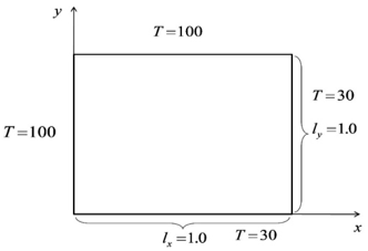
Consider the following problem (Figure 3) on which the algorithm is applied:
The example problem chosen for this implementation is a standard steady-state heat conduction case in a 2D rectangular domain with specified boundary temperatures, thus making it suitable as a test case due to its simplicity and known analytical solution for verification. The domain lengths in x and y direction are one unit each. The boundary conditions used (left and top boundaries at 100 units, right and bottom boundaries at 30 units) represent a realistic gradient commonly seen in thermal systems, where one side is hotter than the other. The grid size (20×20) and the number of random walks (N=2000 per node) were selected to balance the computational efficiency and accuracy; a finer grid or a higher number of random walks would improve the accuracy but increase the computation time. With this setup, the MC method achieves a high degree of agreement with the analytical solution, as can be seen later in this section (97% match for N=2000). This example problem serves as an effective benchmark to validate the Python code and assess solution accuracy across different grid sizes and walks.
Figure 3. Problem definition
The Python program to implement the algorithm discussed above is as follows:
|
from pylab import * from numpy import * # Defining domain $\ell_x$=1 $\ell_y$=1 # Number of nodes nc=20 nr=20 # Spacing between nodes $\Delta$x=$\ell_x$/(nc-1) $\Delta$y=$\ell_y$/(nr-1) # Array of x and y x=linspace(0,$\ell_x$,nc) y=linspace(0,$\ell_y$,nr) # Temperature array T=empty((nr,nc)) # Boundary Condition T[0,:]=100 # Top T[-1,:]=30 # Bottom T[:,0]=100 # Left T[:,-1]=30 # Right # probabilites p_xp=p_xm=p_yp=p_ym=1/4 # Number of random walks N=2000 for i in range(1,nr-1): for j in range(1,nc-1): # initializing $\Sigma$T $\Sigma$T=0 # Starting random walks for ith and jth nodes for rw in range(N): # Resetting of node at this point is must i_node=i j_node=j while True: # Generating random number rn=random.uniform(0,1) # Termination criterion if i_node==0 or i_node==nr-1 or j_node==0 or j_node==nc-1: $\Sigma$T=$\Sigma$T+T[i_node,j_node] break # Direction of random walk elif rn<p_xp: j_node=j_node+1 elif p_xp<rn<p_xp+p_yp: i_node=i_node-1 elif p_xp+p_yp<rn<p_xp+p_yp+p_xm: j_node=j_node-1 else: i_node= i_node+1 # Summing up all the tem's taking their average T[i,j]=$\Sigma$T/N # Data Plotting figure(dpi=300) X,Y=meshgrid(x,flipud(y)) cp=contourf(X,Y,T,20,cmap='jet') colorbar() cp=contour(X,Y,T,10,colors='k') clabel(cp,inline=True, fontsize=10) xlabel('x') ylabel('y') savefig('2D.jpg') |
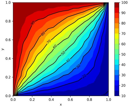
The program output is shown in Figure 4. In the program the number of random walks for each node was taken as 2000. The answer is close to the analytical results.
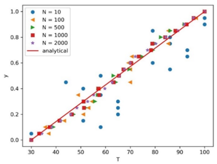
One should be aware that the simulation outcome will never always look exactly like what is depicted above, but rather, there will always be variation, albeit a little amount of variation for a lot of random walks. Figure 5 shows how the solution varies with the variation in the number of random walks, for x=0.5 units, and different y locations.
As observed in Figure 5, the accuracy of the solution improves with the number of random walks, and for N=2000, the statistical output is 97% of the analytical result. The error for 10, 100, 500, 1000, 2000 random walks is also presented in Table 1.
Figure 4. Temperature contour in the domain
Figure 5. Variation of temperature with different random walks
Table 1. Variation of % errors for different random walks
|
y |
10 |
100 |
500 |
1000 |
2000 |
|
1 |
0.00 |
0.00 |
0.00 |
0.00 |
0.00 |
|
0.9 |
7.53 |
-1.51 |
-1.20 |
-0.30 |
-1.20 |
|
0.8 |
0.00 |
-2.44 |
-4.23 |
-2.20 |
-1.99 |
|
0.7 |
17.72 |
-0.89 |
0.18 |
-0.80 |
-2.57 |
|
0.6 |
9.72 |
-3.89 |
-1.94 |
-2.33 |
-2.87 |
|
0.5 |
-10.77 |
0.00 |
-2.80 |
0.65 |
0.70 |
|
0.4 |
-12.07 |
-1.21 |
-1.69 |
-1.57 |
2.96 |
|
0.3 |
27.45 |
6.86 |
9.33 |
0.27 |
3.50 |
|
0.2 |
47.73 |
15.91 |
7.00 |
5.41 |
4.30 |
|
0.1 |
56.76 |
-3.78 |
5.30 |
1.14 |
3.50 |
|
0 |
0.00 |
0.00 |
0.00 |
0.00 |
0.00 |
Table 2. Grid size, random walk and estimated runtime
|
Grid Size |
Random Walks (N) |
Estimated Runtime (s) |
|
10×10 |
1000 |
~2 |
|
10×10 |
2000 |
~4 |
|
20×20 |
1000 |
~8 |
|
20×20 |
2000 |
~15 |
|
20×20 |
5000 |
~35 |
|
40×40 |
1000 |
~30 |
|
40×40 |
2000 |
~55 |
|
40×40 |
5000 |
~138 |
To evaluate the influence of grid refinement on accuracy, a grid convergence study has been conducted. Solutions on progressively finer grids (10×10, 20×20, and 40×40) were compared with the analytical solution, showing a notable increase in accuracy with mesh refinement. For instance, while a 10×10 grid offers an approximation, the 40×40 grid solution aligns closely with analytical values. This convergence comes at a computational cost. Table 2 summarizes the runtime which is associated with each grid size and random walk count (N). For example, with 2000 random walks per node, the runtime on a 20×20 grid is approximately 15 seconds, while the 40×40 grid requires 55 seconds. Doubling the number of random walks to 5000 further increases the runtimes to about 35 seconds and 138 seconds for 20×20 and 40×40 grids respectively. Thus, the choice of grid size and random walk count involves balancing accuracy and efficiency.
In this communication the Monte Carlo (MC) simulation has been employed to model a two-dimensional steady state conduction problem (Laplace equation) with fixed (Dirichlet) boundary constraints. The technique has been presented and is built as an algorithm which is programmed in Python. A numerical problem was used to test the Python code, and it was found that the outcomes are like those of the analytical results. With 2000 random walks, the computed temperature distribution has showed an accuracy of approximately 97% compared to the analytical solution. This has highlighted the effectiveness of the method. Key findings from the study have demonstrated that increasing the number of random walks improves the accuracy of the solution, but at the cost of bigger computational time. For instance, on a 20×20 grid with 2000 random walks per node, the runtime was approximately 15 seconds, while on a 40×40 grid with the same number of random walks, the runtime increased to about 55 seconds.
The developed Python program serves as a effective tool for researchers to understand the application of statistical methods such as MC simulations and provides a basis for developing more complex models. While the study reveals the potential of this approach for solving heat conduction problems, it is important to note that the method’s computational cost grows with grid refinement and the number of random walks, which may limit its scalability for larger problems. The technique also assumes steady-state conditions, restraining its applicability to transient heat conduction problems. Future research could focus on optimizing the random walk algorithm to enhance convergence rates, exploring parallelization strategies to reduce the runtime, and extending the method to handle more complex geometries and transient heat conduction problems. Additionally, further validation against the experimental data and comparison with other numerical methods will strengthen the robustness of this approach.
[1] Bergman, T.L., Lavine, A.S., Incropera, F.P., DeWitt, D.P. (2018). Fundamentals of Heat and Mass Transfer. John Wiley & Sons.
[2] Patankar, S.V. (1980). Numerical Heat Transfer and Fluid Flow. Hemisphere Publishing Corporation. McGraw-Hill.
[3] Deo, A., Joshi, A.R., Parashar, A., Mishra, D.R., Dumka, P. (2022). Analysing one dimensional tapered pin-fin using finite difference. Research and Applications of Thermal Engineering, 5(1): 1-6.
[4] Sizyuk, V., Hassanein, A. (2014). Efficient monte Carlo simulation of heat conduction problems for integrated multi-physics applications. Numerical Heat Transfer, Part B: Fundamentals, 66(5): 381-396. https://doi.org/10.1080/10407790.2014.922850
[5] Zio, E. (2013). Monte Carlo simulation: The method. In: The Monte Carlo Simulation Method for System Reliability and Risk Analysis. Springer Series in Reliability Engineering. Springer, London. https://doi.org/10.1007/978-1-4471-4588-2_3
[6] Harrison, R.L. (2010). Introduction to Monte Carlo simulation. AIP Conference Proceedings, 1204: 17. https://doi.org/10.1063/1.3295638
[7] Gembarovic, J. (2017). Using Monte Carlo simulation for solving heat conduction problems, ResearchGate Preprint, 1-25. https://doi.org/10.13140/RG.2.2.20591.64162
[8] Dumka, P., Gajula, K., Sharma, V., Mishra, D.R. (2022). Modelling pipe flow using Python. International Education & Research Journal, 8(10): 4-7. https://www.researchgate.net/publication/364385651_MODELLING_PIPE_FLOW_USING_PYTHON.
[9] Dumka, P., Dumka, R., Mishra, D.R. (2022). Numerical Methods Using Python. Blue Rose Publishers. https://books.google.co.in/books/about/Numerical_Methods_using_Python_For_scien.html?id=zRWdEAAAQBAJ&redir_esc=y.
[10] Joshi, A.R., Deo, A., Parashar, A., Mishra, D.R., Dumka, P. (2023). Modelling steam power cycle using Python. International Journal of Scientific Research in Computer Science, Engineering and Information Technology (IJSRCSEIT), 9(1): 152-162. https://doi.org/10.32628/CSEIT228671
[11] Dumka, P., Mishra, D.R. (2022). Understanding the TDMA/Thomas algorithm and its Implementation in Python. International Journal of All Research Education and Scientific Methods, 10(10): 998-1002.
[12] Dumka, P., Pawar, P.S., Sauda, A., Shukla, G., Mishra, D.R. (2022). Application of He's homotopy and perturbation method to solve heat transfer equations: A Python approach. Advances in Engineering Software, 170: 103160. https://doi.org/10.1016/j.advengsoft.2022.103160
[13] Backer, A. (2007). Computational physics education with Python. Computing in Science & Engineering, 9(3): 30-33. https://doi.org/10.1109/MCSE.2007.48
[14] Dumka, P., Chauhan, R., Singh, A., Singh, G., Mishra, D. (2022). Implementation of Buckingham's Pi theorem using Python. Advances in Engineering Software, 173: 103232. https://doi.org/10.1016/j.advengsoft.2022.103232
[15] Dumka, P., Rana, K., Tomar, S.P.S., Pawar, P.S., Mishra, D.R. (2022). Modelling air standard thermodynamic cycles using Python. Advances in Engineering Software, 172: 103186. https://doi.org/10.1016/j.advengsoft.2022.103186
[16] Ranjani, J., Sheela, A., Meena, K.P. (2019). Combination of NumPy, SciPy and Matplotlib/Pylab-A good alternative methodology to MATLAB-A Comparative analysis. In 2019 1st International Conference on Innovations in Information and Communication Technology (ICIICT), Chennai, India, pp. 1-5. https://doi.org/10.1109/ICIICT1.2019.8741475
[17] Bauckhage, C. (2020). NumPy/SciPy recipes for data science: Subset-constrained vector quantization via mean discrepancy minimization, 1-4.
[18] Porcu, V. (2018). Matplotlib. In: Python for Data Mining Quick Syntax Reference. Apress, Berkeley, CA. https://doi.org/10.1007/978-1-4842-4113-4_10
[19] Bisong, E., Bisong, E. (2019). Matplotlib and seaborn. In Building Machine Learning and Deep Learning Models on Google Cloud Platform: A Comprehensive Guide for Beginners, Apress, Berkeley, CA, pp. 151-165. https://doi.org/10.1007/978-1-4842-4470-8_12
[20] Dumka, P., Chauhan, R., Mishra, D.R., Shaik, F., Govindaraj, P., Kumar, A., Sonawane, C., Velkin, V.I. (2024). Development and implementation of a Python functions for automated chemical reaction balancing. Indonesian Journal of Electrical Engineering and Computer Science, 34(3): 1557-1565. https://doi.org/10.11591/ijeecs.v34.i3.pp1557-1565