Yanwen Yu![]() | Hefei Hu*
| Hefei Hu*![]()
© 2025 The authors. This article is published by IIETA and is licensed under the CC BY 4.0 license (http://creativecommons.org/licenses/by/4.0/).
OPEN ACCESS
With the rise of applications such as the Internet of Things (IoT) and Virtual Reality (VR), there is an increasing demand for stringent service latency and quality of service requirements, which has led to a shift in network service deployment from cloud to edge, giving rise to Mobile Edge Computing (MEC) architectures. In MEC environments, network infrastructure is distributed near users, allowing access to local networks in real time. However, dynamically orchestrating Service Function Chains (SFCs) presents a significant challenge, especially in resource-constrained settings where maximizing SFC deployments while maintaining low latency is essential for service providers’ revenue optimization. To address this challenge, this paper proposes an intelligent SFC orchestration strategy, termed GCN-DQN, which combines Graph Convolutional Networks (GCNs) and Deep Q-Networks (DQNs). The GCN-DQN framework is designed to optimize the request acceptance rate while ensuring compliance with stringent low-latency requirements. To achieve this, the GCN-DQN strategy is designed to perceive network structure, resource availability, and SFC-specific information, enabling optimized decision-making for SFC traffic steering paths. Performance evaluations demonstrate that the proposed algorithm outperforms existing methods in SFC request acceptance rates under various network loads.
Mobile Edge Computing, Service Function Chains, Graph Convolutional Networks, Deep Q-Networks, performance consistency across networks, traffic steering optimization
The advent of network virtualization and cloud computing has positioned service function chaining [1] as a pivotal technology for the dynamic deployment and management of sequential network functions—such as firewalls, load balancers—tailored to specific service requirements. Traditionally, these functions have been statically deployed within networks, resulting in limited flexibility and adaptability. Nevertheless, as network traffic continues to surge and application scenarios grow increasingly complex, the challenge of intelligent and dynamic SFC deployment has emerged as a crucial concern in modern network management.
Recent advances in deep reinforcement learning [2] have demonstrated considerable potential in tackling decision-making challenges, particularly in the dynamic deployment of SFCs. Nonetheless, a key limitation of many DRL-based approaches in network environments is their restricted generalizability. While these methods perform effectively on network topologies encountered during training, their performance significantly deteriorates when applied to novel, unseen topologies. This limitation stems from the use of conventional neural networks—such as fully connected and convolutional networks—that are not inherently equipped to process graph-structured data. In recent years, graph neural networks [3], a deep learning model designed to process graph-structured data, have shown exceptional performance in areas such as social network analysis, molecular modeling, and recommendation systems. GNNs effectively capture the complex relationships and dependencies between nodes, offering a unique advantage for addressing SFC deployment challenges. By leveraging GNNs, it is possible to efficiently deploy SFCs in complex network topologies, optimizing network resource utilization while satisfying quality of service [4] requirements.
To tackle the challenge of intelligent SFC orchestration in Mobile Edge Computing (MEC) [5-8] environments, where user mobility significantly influences SFC deployment, this paper introduces a 0-1 Integer Linear Programming model for dynamic SFC orchestration. Leveraging this model, we propose a GCN-DQN-based framework designed to intelligently determine traffic steering paths, thereby enhancing the acceptance rate of SFC requests. The main contributions of this paper are outlined below:
A considerable body of research has focused on the deployment of Service Function Chains (SFC). Given our objective of deploying as many SFCs as possible in a Mobile Edge Computing (MEC) environment with limited resources, we closely monitor each SFC traffic steering path to optimize the overall request acceptance rate within the network. Traditional optimization techniques, including exact methods, heuristics [9], and meta-heuristics [10], encounter significant limitations as the solution space expands exponentially with the growth of the state space, rendering them less effective in complex network environments. In contrast, Deep Reinforcement Learning (DRL) has emerged as a potent approach for autonomously deriving optimal decision-making strategies while maximizing long-term rewards. By integrating the perceptive capabilities of deep learning with the strategic strengths of reinforcement learning, DRL learns directly from experience, enabling a deeper understanding of both the network and tasks, thereby improving accuracy and minimizing the need for repetitive modeling.
Owing to its self-learning and online learning capabilities, DRL presents a promising solution for facilitating dynamic adjustments in SFC orchestration optimization. Consequently, this paper reviews the state-of-the-art from two perspectives: DRL-based SFC orchestration utilizing traditional neural networks, such as Convolutional Neural Networks (CNNs) and Recurrent Neural Networks (RNNs), and DRL-based SFC orchestration employing Graph Neural Networks.
2.1 DRL approaches based on traditional neural networks
According to the study of Fu et al. [11], the Virtual Network Function (VNF) problem is broken down into individual VNF components and an internal connection graph, forming a VNF forwarding graph. The SFC embedding challenge is then framed as a Deep Reinforcement Learning (DRL) problem, enabling effective solutions to complex and dynamic environments.
As reported by Li et al. [12], the task of mapping SFCs with varying priorities onto the fundamental network is formulated as a multi-step Integer Linear Programming problem with distinct objectives. A DQN-based mapping approach is proposed, wherein the DRL agent selects between two straightforward SFC mapping strategies.
As demonstrated by Liu et al. [13], a dynamic SFC orchestration framework for Internet of Things (IoT) networks is proposed, specifically designed for DRL-enabled IoT environments. This framework can address the SFC dynamic orchestration problem in dynamic and complex network scenarios.
In the study conducted by Wang et al. [14], the DDQP and its extension, DDQP+ algorithms, are designed for real-time deployment of primary and backup SFC instances. These algorithms provide continuous state updates from active instances to backup instances for stateful VNFs, ensuring seamless redirection in the event of a failure.
The aforementioned DRL-based approaches predominantly rely on simple neural network architectures, such as feedforward and recurrent neural networks. However, these architectures are limited in their capacity to effectively capture features from the underlying network structure. Traditional DRL methods, including those utilizing Convolutional Neural Networks and Recurrent Neural Networks, encounter significant challenges when applied to complex, highly dynamic environments like Mobile Edge Computing (MEC). These models often struggle to capture the intricate relationships and dependencies between network elements. Additionally, these methods lack generalization capability across different network topologies.
To overcome these challenges, recent studies have started to explore DRL combined with Graph Neural Networks. GNNs are well-suited for representing the topological structure of networks, making them ideal for optimizing SFC orchestration in MEC environments. By using GNNs, DRL-based SFC orchestration can more effectively model the interactions between network components, leading to improved performance in terms of scalability, adaptability, and resource utilization.
2.2 DRL approaches based on graph neural networks
The findings of Sun et al. [15] suggested that a combination of Graph Neural Network (GNN) and DQN is used to optimize Virtual Network Function (VNF) placement. The GNN module maps node features to adjacent edges, which are then aggregated and re-encoded into the node features. Input attributes include the processing and storage utilization of network nodes, while edge attributes are represented by bandwidth usage and latency of network links. The output is a binary list indicating selected nodes, and the shortest path algorithm is applied to deploy routing paths between VNFs.
Based on the study presented by Heo et al. [16], a sequence model based on Graph Neural Networks is proposed for VNF placement. This model consists of a graph encoder, which represents the network topology, and a decoder, which computes the probabilities for adjacent nodes and VNF execution.
In the study conducted by Qi et al. [17], a service function chain with a graph structure is considered, and various SFC graph structures are modeled using a Graph Convolutional Network. The aim is to handle diverse SFC graph structures. The DDQN algorithm is employed to make decisions regarding the server index for the current VNF deployment.
All of the above studies, however, do not take into account the traffic paths between VNFs and deploy them by utilizing the shortest path algorithm. While the shortest path algorithm maximizes immediate rewards in the current network state, it is not the optimal choice for long-term network environments.
According to the research by Xiao et al. [18], a two-stage GCN-assisted DRL framework is introduced to optimize SFC request acceptance while minimizing network costs. In the first stage, the upper-layer Management and Orchestration (MANO) agent collaborates with lower-layer MANOs to define the local observation scopes for each agent. The second stage operates within a discrete time-slot system, where resources occupied by expired SFCs are released at the beginning of each time slot, and all lower-layer MANOs simultaneously begin embedding new SFCs. This study only investigates the migration of SFCs between different nodes and does not design specific VNF deployment strategies or routing path selection, thus not addressing the practical SFC deployment problem.
Our proposed GCN-DQN method builds upon these advancements, combining the strengths of Graph Convolutional Networks and Deep Q-Networks to optimize SFC traffic steering paths. It not only addresses the limitations of DRL but also makes decisions for SFC traffic paths, thereby solving the practical SFC deployment problem.
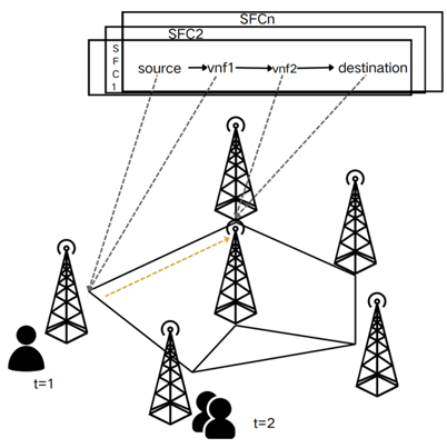
Figure 1 illustrates the dynamic SFC orchestration model in MEC environments. The model is organized hierarchically, starting with the network function virtualization infrastructure (NFVI) at the bottom, followed by virtual network functions (VNFs), and ending with user services. The process concludes with the delivery of user services, enabling users to seamlessly roam across various NFVIs. Therefore, it is necessary to dynamically orchestrate the deployment locations of SFCs and the corresponding traffic steering paths.
In the practical problem, a time-slot model is designed where SFC requests arrive dynamically. As shown in Figure 1, at t=1, only User 1 submits a service request. At t=2, Users 2 and 3 join the network. Over time, more users will enter the network, and some users will leave.
Figure 1. Intelligent SFC orchestration model
3.1 Network function virtualization infrastructure
The NFVI model is represented as an undirected graph $\mathrm{G}^s=$ $\left(\mathrm{N}^s, \mathrm{E}^s\right)$, where $\mathrm{N}^s$ denotes the set of physical nodes, $\mathrm{N}^s=$ $\left(\mathrm{N}_{\mathrm{A}}^s \cup \mathrm{~N}_{\mathrm{E}}^s\right.$ ) including access nodes $\mathrm{N}_{\mathrm{A}}^s$ and edge computing nodes $\mathrm{N}_{\mathrm{E}}^s$. Each edge computing node has constrained resources, denoted by $R$, which include resource types such as $C P U$, storage, and others. For any given resource $r \in R$, $\operatorname{cap}^{\mathrm{r}}\left(\mathrm{n}_{\mathrm{i}}^s\right)$ denotes the quantity of resource type r available at node $n_i^s$. The set of physical links is denoted by $\mathrm{E}^s$, where each link $e_{i j}^s \in E^s$ connects adjacent nodes $n_i^s$ and $n_j^s$. Each link $e_{i j}^s$ has associated bandwidth $\mathrm{bw}\left(\mathrm{e}_{\mathrm{ij}}^{\mathrm{s}}\right)$ and latency delay $\left(e_{\mathrm{ij}}^{\mathrm{s}}\right)$. It is assumed that the service requirements can be met by the sufficiently large internal bandwidth of each edge computing node [19].
3.2 Virtual network functions
VNFs are software-based components designed to perform a variety of traffic processing tasks within edge computing nodes. We hypothesize a linear relationship between traffic volume and the corresponding resource requirements [20], let $V$ denote the set of VNF types, where $\mathrm{f}_\mathrm{i} \in F$ represents a specific type of VNF capable of providing particular traffic processing services. Given the varying resource consumption across different VNF types. The resource demand coefficient coeff${ }^{\mathrm{r}}\left(\mathrm{f}_{\mathrm{i}}\right)$ indicates the quantity of resource type r required for a unit size of traffic processed by the VNF $\mathrm{f}_\mathrm{i}$. Additionally, since VNFs handle packets in different ways, such as adding headers, these processes can modify the traffic size [21]. We define this alteration as the traffic scaling factor ratio $\left(\mathrm{f}_\mathrm{i}\right)$ of the virtual network function $\mathrm{f}_\mathrm{i}$.
3.3 User services
In Mobile Edge Computing (MEC), as a user's location may vary over time. Consequently, the source node of the Service Function Chain changes dynamically. we adopt a discrete, periodic stationary time-slot model t $\in$ {1,2,3...} to simplify the problem, where the user service access nodes remain stationary within each time slot and switching occurs between time slots.
The user service demands across the network can be represented as a set of Service Function Chains (SFCs) Gv, where $G_j^v \in G^v$ denotes the $j$-th SFC. A directed graph $G_j^v=$ $\left(\mathrm{N}_{\mathrm{j}}^{\mathrm{v}}, \mathrm{E}_{\mathrm{j}}^v\right)$ represents source nodes, an ordered set of network functional requirements, and destination nodes. Let $\mathrm{N}_{\mathrm{j}}^{\mathrm{v}}=$ $\left\{S_j, n_{j 1}^v \ldots n_{j 1}^v \ldots D_j\right\}, S_j(t)$ represent the source node at time $t$ and $n_{\mathrm{ji}}^{\mathrm{v}}\left(1 \leq \mathrm{i} \leq\left|\mathrm{N}_{\mathrm{j}}^{\mathrm{v}}\right|-1\right)$ is defined as the type of VNF of type $f\left(n_{j i}^v\right) \in F$ that needs to be mapped to an edge compute node for traffic passing through the i-th network function. $D_j(t)$ represents the destination node at time $t$. Let $E_j^v$ denote the set of virtual links, where $e_{\mathrm{ji}}^{\mathrm{v}} \in \mathrm{E}_{\mathrm{j}}^{\mathrm{v}}$ represents the virtual link between adjacent VNFs $n_{j i}^v$ and $n_{j(i+1)}^{\mathrm{v}}$. For simplification, we denote the source node as $\mathrm{n}_{\mathrm{j} 0}^{\mathrm{v}}$ and the destination node as $n_{j\left|N_j^v\right|-1}^v$. For any given SFC $G_j^v, D\left(G_j^v\right)$ and $F\left(G_j^v\right)$ represent the target latency requirement and the traffic demand, respectively. Based on the required network function types and traffic sizes for the SFC, the virtual links' bandwidth requirement is given by Eq. (1):
$\begin{gathered}\operatorname{traffic}\left(\mathrm{e}_{\mathrm{ji}}^{\mathrm{v}}\right)=\mathrm{F}\left(\mathrm{G}_{\mathrm{j}}^{\mathrm{v}}\right) \cdot \prod_{\mathrm{x}=0}^{\mathrm{i}} \operatorname{ratio}\left(\mathrm{f}\left(\mathrm{n}_{\mathrm{jx}}^{\mathrm{v}}\right)\right)\left(\operatorname{ratio}\left(\mathrm{f}\left(\mathrm{n}_{\mathrm{j} 0}^{\mathrm{v}}\right)\right)=1\right)\end{gathered}$ (1)
Therefore, we can express the demand for the resource of type r (r $\in$ R) by the network function $n_{\text{ji}}^\text{v}$ as Eq. (2):
$\begin{aligned} & \operatorname{res}^r\left(n_{j i}^v\right)=\operatorname{coeff}^r\left(f\left(n_{j i}^v\right)\right) \cdot \operatorname{traffic}\left(e_{j(i-1)}^v\right)=\operatorname{coeff}^r\left(f\left(n_{j i}^v\right)\right) \cdot F\left(G_j^v\right) \cdot \prod_{x=0}^{i-1} \operatorname{ratio}\left(f\left(n_{j x}^v\right)\right)\end{aligned}$ (2)
3.4 Network latency
The rapid development of MEC is attributed to its ability to provide services in close proximity, significantly reducing service latency. Compared to cloud networks, the distributed NFVI, limited computing resources, and link bandwidth in edge computing environments necessitate consideration of both link propagation delay and queuing delay, as represented by Eq. (3):
$\operatorname{delay}\left(\mathrm{e}_{\mathrm{ij}}^{\mathrm{s}}\right)=$ prop_delay $\left(\mathrm{e}_{\mathrm{ij}}^{\mathrm{s}}\right)+$ queue_dealy $\left(\mathrm{e}_{\mathrm{ij}}^{\mathrm{s}}\right)$ (3)
The propagation delay prop_delay$\left(\mathrm{e}_{\mathrm{ij}}^{\mathrm{s}}\right)$ refers to the time taken for information to travel across a communication medium, which is proportional to the length of the medium. Queuing delay queue_dealy$\left(e_{\mathrm{ij}}^{\mathrm{s}}\right)$ is the time a packet waits in the queue, which is related to the current link traffic. The queuing delay is modeled using the M/M/1 queuing model [22], which is defined as the ratio of the remaining bandwidth of the link. The calculation of the queuing delay, based on this model, is presented in Eq. (4):
queue_dealy $\left(\mathrm{e}_{\mathrm{ij}}^{\mathrm{s}}\right)=\mathrm{d}_{\mathrm{ij}} \cdot\left(1-\omega_{\mathrm{ij}}(\mathrm{t}) / \omega_{\mathrm{ij}}(\mathrm{t})\right)$ (4)
where, $\mathrm{d}_{\mathrm{ij}}$ denotes the transmission delay of a single data packet.
3.5 Traffic steering
Most Commonly Used SFC The most widely used algorithm for traffic steering is the shortest path algorithm. While it effectively minimizes service latency and optimizes network bandwidth, it is not without its inherent limitations. This study builds upon the shortest path approach to consider more feasible traffic steering paths. Let $\tau_{\mathrm{pq}}$ denote the first k shortest propagation delay paths between nodes $\mathrm{n}_{\mathrm{p}}^s$ and $\mathrm{n}_{\mathrm{q}}^{\mathrm{s}}$, where $\tau_{\mathrm{pql}}$ represents the 1-th $\left(1 \leq 1 \leq\left|\tau_{\mathrm{pq}}\right|\right)$ path. For computational convenience, we define a binary variable $\sigma_{\mathrm{pql}}^{\mathrm{ji}}$ to indicate whether a link $\mathrm{e}_{\mathrm{ij}}^{\mathrm{s}}$ is included in $\tau_{\mathrm{pql}}$. The latency of the traffic steering path is given by:
\begin{array}{c} \mathrm{d}_{\mathrm{pq1}}(\mathrm{t})=\sum_{\mathrm{e}_{\mathrm{ij}} \in\mathrm{E}^{\mathrm{s}}}\sigma_{\mathrm{pql}}^{\mathrm{ji}}\cdot\operatorname{delay}\left(\mathrm{e}_{\mathrm{ij}}^{\mathrm{s}}\right)=\sum_{\mathrm{e}_{\mathrm{ij}}^{\mathrm{j}}=\mathrm{E}^{\mathrm{s}}} \sigma_{\mathrm{pql}}^{\mathrm{ji}}\cdot\left(\operatorname{prop}_{\text {delay }\left(\mathrm{e}_{\mathrm{ij}}^{\mathrm{s}}\right)}+\text { queue }_{\text{dealy}\left(\mathrm{e}_{\mathrm{ij}}^{\mathrm{s}}\right)}\right)\\=\sum_{\mathrm{e}_{\mathrm{ij}}^{\mathrm{i}}=\mathrm{E}^{\mathrm{i}}} \sigma_{\mathrm{pql}}^{\mathrm{ii}} \cdot \operatorname{prop}_{\text {delay }\left(e_{\mathrm{ij}}^{\mathrm{s}}\right)}+\sum_{e_{i j} \in\mathrm{E}^{\mathrm{s}}} \sigma_{\mathrm{pql}}^{\mathrm{ji}} \cdot \mathrm{~d}_{\mathrm{ij}} \cdot\left(1-\omega_{\mathrm{ij}}(\mathrm{t}) / \omega_{\mathrm{ij}}(\mathrm{t})\right)\end{array} (5)
$\begin{aligned} \mathrm{d}_{\mathrm{pql}}(\mathrm{t})= & \sum_{\mathrm{e}_{\mathrm{ij}}^{\mathrm{s}} \in \mathrm{E}^{\mathrm{s}}} \sigma_{\mathrm{pql}}^{\mathrm{ji}} \cdot \operatorname{delay}\left(\mathrm{e}_{\mathrm{ij}}^{\mathrm{s}}\right)=\sum_{\mathrm{e}_{\mathrm{ij}}^{\mathrm{s}} \in \mathrm{E}^{\mathrm{s}}} \sigma_{\mathrm{pq1}}^{\mathrm{ji}} \cdot\left(\operatorname{prop}_{\text {delay }\left(\mathrm{e}_{\mathrm{ij}}^{\mathrm{s}}\right)}+\text { queue }_{\text {dealy }\left(\mathrm{e}_{\mathrm{ij}}^{\mathrm{s}}\right)}\right) \\ & =\sum_{\mathrm{e}_{\mathrm{ij}}^{\mathrm{s}} \in \mathrm{E}^{\mathrm{s}}} \sigma_{\mathrm{pql}}^{\mathrm{ji}} \cdot \operatorname{prop}_{\text {delay }\left(\mathrm{e}_{\mathrm{ij}}^{\mathrm{s}}\right)}+\sum_{\mathrm{e}_{\mathrm{ij}}^{\mathrm{s} \in E^s}} \sigma_{\mathrm{pql}}^{\mathrm{ji}} \cdot \mathrm{d}_{\mathrm{ij}} \cdot\left(1-\omega_{\mathrm{ij}}(\mathrm{t}) / \omega_{\mathrm{ij}}(\mathrm{t})\right)\end{aligned}$ (5)
In Eq. (5), the first term represents the sum of the propagation delays of the adjacent links in the traffic steering path, which is constant. The second term is the sum of the queuing delays across all adjacent links, dependent on the traffic load. The paths in the set are ordered by propagation delay in ascending order, meaning that paths ranked higher are shorter and traverse fewer routes. Let traffic steering paths between all nodes in the network be denoted by $\Gamma\left(\tau_{11}, \tau_{12} \ldots \tau_{\mathrm{pq}} \ldots\right)$. The SFC traffic steering will take all these paths into account.
3.6 Decision model and optimization objectives
In the MEC environment, considering the dynamic arrival of users and their mobility, the SFC dynamic orchestration problem can be viewed as mapping directed graph $\text{G}^v$ sets at each time slot t to the undirected graph $\text{G}^s$ of the NFVI. The mapping of user services to the NFVI must account for both the variations in service latency due to user mobility and the resource constraints of the NFVI, ensuring efficient resource utilization to prevent network congestion. To address this issue, a 0-1 Integer Linear Programming model has been developed for SFC dynamic orchestration in the MEC environment, and Boolean decision variables $\zeta_\text{ji}^{\mathrm{p}}(\mathrm{t})$ and $\eta_{\mathrm{ji}}^{\mathrm{pq}}(\mathrm{t})$ are defined as follows:
$\zeta_{\mathrm{ji}}^{\mathrm{p}}(\mathrm{t})=\left\{\begin{array}{c}1 \text { if } \mathrm{n}_{\mathrm{ji}}^{\mathrm{v}} \text { is mapped to } \mathrm{n}_{\mathrm{p}}^s \text { in the time } \mathrm{t} \\ 0 \text { if } \mathrm{n}_{\mathrm{ji}}^{\mathrm{v}} \text { is not mapped to } \mathrm{n}_{\mathrm{p}}^s \text { in the time } \mathrm{t}\end{array}\right.$ (6)
$\eta_{\mathrm{ji}}^{\mathrm{pql}}(\mathrm{t})=\left\{\begin{array}{c}1 \text { if } \mathrm{e}_{\mathrm{ji}}^{\mathrm{V}} \text { is mapped to } \tau_{\mathrm{pql}} \text { in the time } \mathrm{t} \\ 0 \text { if } \mathrm{e}_{\mathrm{ji}}^{\mathrm{v}} \text { is not mapped to } \tau_{\mathrm{pql}} \text { in the time } \mathrm{t}\end{array}\right.$ (7)
In time t, where $\eta_{\mathrm{ji}}^{\mathrm{pql}}(\mathrm{t})$ denotes whether the virtual link $\mathrm{e}_{\mathrm{ji}}^{\mathrm{v}}$ in the SFC $\mathrm{G}_{\mathrm{j}}^{\mathrm{v}}$ is mapped in the path set $\tau_{\mathrm{pql}}$, and $\zeta_{\mathrm{ji}}^{\mathrm{p}}(\mathrm{t})$ denotes whether the i-th virtual network function $\mathrm{n}_{\mathrm{ji}}^{\mathrm{v}}$ in the SFC $\mathrm{G}_{\mathrm{j}}^{\mathrm{v}}$ is mapped to the physical node.
Based on the aforementioned decision variables, in the time t, the remaining bandwidth ratio $\omega_{\mathrm{mn}}$ of the link $\mathrm{e}_{\mathrm{mn}}^{\mathrm{s}}$ is given by Eq. (8):
$\omega_{\mathrm{mn}}(\mathrm{t})=1-\sum_{\mathrm{G}_{\mathrm{j}}^{\mathrm{v}} \in G^{\mathrm{v}}} \sum_{\mathrm{e}_{\mathrm{ji}} \in G_{\mathrm{j}}^{\mathrm{v}}}\left(\sum_{\tau_{\mathrm{pq}} \in \Gamma} \sum_{\tau_{\mathrm{pql}} \in \tau_{\mathrm{pq}}} \operatorname{traffic}\left(\mathrm{e}_{\mathrm{ji}}^{\mathrm{v}}\right)\right.\left.\cdot \eta_{\mathrm{ji}}^{\mathrm{pql}}(\mathrm{t}) \cdot \sigma_{\mathrm{pql}}^{\mathrm{mn}}\right) / \mathrm{bw}\left(\mathrm{e}_{\mathrm{mn}}^{\mathrm{s}}\right)$ (8)
Therefore, the total service latency of the SFC $\text{G}_j^v$ is given by Eq. (9):
$\mathrm{d}_{\mathrm{j}}(\mathrm{t})=\sum_{\mathrm{e}_{\mathrm{j} i} \in \mathrm{E}_{\mathrm{j}}^{\mathrm{v}}} \sum_{\tau_{\mathrm{pq} 1} \in \tau_{\mathrm{pq}}} \eta_{\mathrm{ji}}^{\mathrm{pql}}(\mathrm{t}) \cdot \mathrm{d}_{\mathrm{pql}}(\mathrm{t})$ (9)
The total latency of the SFC is given by Eq. (10):
$\mathrm{d}(\mathrm{t})=\sum_{\mathrm{G}_{\mathrm{j}}^{\mathrm{v}} \in \mathrm{G}^{\mathrm{v}}} \mathrm{d}_{\mathrm{j}}(\mathrm{t})$ (10)
The number of SFC requests received is given by Eq. (11):
$\begin{array}{c} A(t)=\sum_{G_j^v \in G^v} f\left(\left(\sum_{n_{j i}^v \in G_j^V} \sum_{n_p^s \in N^s} \zeta_{j i}^p(t)-\left|N_j^v\right|\right)\right. \\ \left.+\left(\sum_{\mathrm{e}_{\mathrm{j} i} \in E_{\mathrm{j}}^{\mathrm{V}}} \sum_{\mathrm{\tau pq}_{\mathrm{pq}} \in \Gamma} \sum_{\tau_{\mathrm{pq} 1} \in \tau_{\mathrm{pq}}} \sum_{\mathrm{e}_{\mathrm{mn}}^{\mathrm{s}} \in \mathrm{E}^{\mathrm{s}}} \eta_{\mathrm{ji}}^{\mathrm{pql}}(\mathrm{t}) \cdot \sigma_{\mathrm{pql}}^{\mathrm{mn}}-\left(\left|N_{\mathrm{j}}^{\mathrm{V}}\right|-1\right)\right)\right)\end{array}$ (11)
where, $f(x)=\left\{\begin{array}{l}0, x<0 \\ 1, x \geq 0\end{array}\right.$.
This paper aims to optimize the overall acceptance rate of SFC requests, ensuring that the constraints on physical resources and latency within the NFVI are satisfied. Therefore, the optimization objective is:
$\operatorname{MaximizeA}(\mathrm{t})-\mathrm{d}(\mathrm{t})$ (12)
To unify the positive and negative meanings of the optimization objective, this paper adopts the latency optimization rate $\emptyset(t)$ as the final optimization criterion:
$\emptyset(\mathrm{t})=\sum_{\mathrm{G}_{\mathrm{j}}^{\mathrm{v}} \in \mathrm{G}^{\mathrm{v}}}\left(\mathrm{D}\left(\mathrm{G}_{\mathrm{j}}^{\mathrm{v}}\right)-\mathrm{d}_{\mathrm{j}}(\mathrm{t})\right) /\left(\mathrm{D}\left(\mathrm{G}_{\mathrm{j}}^{\mathrm{v}}\right)\right.$ (13)
Therefore, the final optimization objective is:
$\operatorname{MaximizeA}(\mathrm{t})+\emptyset(\mathrm{t})$ (14)
In Mobile Edge Computing (MEC) environments, service providers typically aim to accept as many SFC requests as possible while optimizing services under limited resources. Therefore, choosing "maximizing the request acceptance rate" as the objective function aligns with practical needs, effectively evaluating and enhancing the overall efficiency of SFC traffic steering paths. Due to the resource constraints in MEC environments, in addition to maximizing the request acceptance rate, it is also essential to ensure low latency and service quality. This is another basis for the design of the objective function, ensuring system stability and user satisfaction.
In SFC orchestration, the mapping of source and destination nodes is a critical constraint, as it ensures that service requests can be correctly transmitted from the source node to the destination node, maintaining network connectivity and data flow integrity. The mapping of virtual nodes and virtual links to the physical topology is necessary to support the functional requirements of the virtual network and avoid conflicts or wastage of physical resources. Node resources as constraints ensure that virtual nodes can be mapped to physical nodes with sufficient computational, storage, and processing capabilities, thus preventing resource overload and ensuring system stability. Link resource constraints ensure that virtual links can be mapped to physical links that meet bandwidth requirements, enabling efficient data flow transmission. These constraints ensure the rational allocation of resources, improve the utilization efficiency of network resources, and optimize service quality. Therefore, the constraint conditions are as follows:
The SFC source node’ mapping location must be the user access node, and the mapping location of the SFC endpoint must be the destination node:
$\begin{gathered}\zeta_{\mathrm{j0}}^{\mathrm{p}}(\mathrm{t})=\mathrm{S}_{\mathrm{j}}(\mathrm{t}), \quad \forall \mathrm{G}_{\mathrm{j}}^{\mathrm{v}} \in \mathrm{G}^{\mathrm{v}} \\ \zeta_{\mathrm{j}\left(\left|\mathrm{N}_{\mathrm{j}}^{\mathrm{v}}\right|-1\right)}^{\mathrm{p}}(\mathrm{t})=\mathrm{D}_{\mathrm{j}}(\mathrm{t}), \quad \forall \mathrm{G}_{\mathrm{j}}^{\mathrm{v}} \in \mathrm{G}^{\mathrm{v}}\end{gathered}$ (15)
In any time slot t, all virtual network functions used by the SFC must be deployed:
$\sum_{\mathrm{n}_{\mathrm{p}}^{\mathrm{s}} \in \mathrm{N}^{\mathrm{s}}} \zeta_{\mathrm{ji}}^{\mathrm{p}}(\mathrm{t})=1, \quad \forall \mathrm{G}_{\mathrm{j}}^{\mathrm{v}} \in \mathrm{G}^{\mathrm{v}}, \forall \mathrm{n}_{\mathrm{ji}}^{\mathrm{v}} \in \mathrm{G}_{\mathrm{j}}^{\mathrm{v}}$ (16)
In any time slot t, all virtual links used by the SFC must be deployed:
$\sum_{\tau_{\mathrm{pq}} \in \Gamma} \sum_{\tau_{\mathrm{pql}} \in \tau_{\mathrm{pq}}} \sum_{\mathrm{e}_{\mathrm{mn}} \in \mathrm{E}^{\mathrm{s}}} \eta_{\mathrm{ji}}^{\mathrm{pql}}(\mathrm{t}) \cdot \sigma_{\mathrm{pql}}^{\mathrm{mn}}=1,\forall \mathrm{G}_{\mathrm{j}}^{\mathrm{v}} \in \mathrm{G}^{\mathrm{v}}, \forall \mathrm{e}_{\mathrm{ji}}^{\mathrm{v}} \in \mathrm{G}_{\mathrm{j}}^{\mathrm{v}}$ (17)
In any time slot t, the resource constraints of the edge computing nodes in the NFVI are as follows:
$\begin{gathered}\sum_{\mathrm{G}_{\mathrm{i}}^{\mathrm{V}} \in \mathrm{G}^{\mathrm{v}}} \sum_{\mathrm{n}_{\mathrm{ij}}^{\mathrm{v}} \in G_{\mathrm{i}}^{\mathrm{v}}} \operatorname{res}^{\mathrm{r}}\left(\mathrm{n}_{\mathrm{ji}}^{\mathrm{v}}\right) \cdot \zeta_{\mathrm{ji}}^{\mathrm{p}}(\mathrm{t}) \leq \operatorname{cap}^{\mathrm{r}}\left(\mathrm{n}_{\mathrm{p}}^{\mathrm{s}}\right), \forall \mathrm{n}_{\mathrm{p}}^{\mathrm{s}} \in \mathrm{N}_{\mathrm{E}}^{\mathrm{s}}, \forall \mathrm{r} \in \mathrm{R}\end{gathered}$ (18)
In any time slot t, the bandwidth constraints of the physical links in the NFVI are as follows:
$\sum_{\mathrm{G}_{\mathrm{j}}^{\mathrm{v}} \in \mathrm{G}^{\mathrm{v}}} \sum_{\mathrm{e}_{\mathrm{ji}}^{\mathrm{v}} \in G_{\mathrm{j}}^{\mathrm{v}}}\left(\sum_{\tau_{\mathrm{pq}} \in \Gamma} \sum_{\tau_{\mathrm{pq} 1} \in \tau_{\mathrm{pq}}} \operatorname{traffic}\left(\mathrm{e}_{\mathrm{ji}}^{\mathrm{v}}\right) \cdot \eta_{\mathrm{ji}}^{\mathrm{pql}}(\mathrm{t}) \cdot \sigma_{\mathrm{pql}}^{\mathrm{mn}}\right) \leq \operatorname{bw}\left(\mathrm{e}_{\mathrm{mn}}^{\mathrm{s}}\right), \forall \mathrm{e}_{\mathrm{mn}}^{\mathrm{s}} \in \mathrm{E}^{\mathrm{s}}$ (19)
We propose the GCN-DQN framework, which integrates Graph Convolutional Networks with Deep Q-Networks to optimize Service Function Chain traffic steering paths in Mobile Edge Computing environments. The rationale behind combining GCNs and DQNs lies in their complementary strengths: GCNs are well-suited to model the network's topological structure, capturing the complex relationships between nodes, while DQNs excel in decision-making by learning from past experiences to optimize long-term rewards. In the context of MEC, where the network topology is dynamic and highly complex, this combination allows the GCN-DQN framework to not only understand the intricate dependencies between network elements but also adapt and optimize traffic steering paths in real-time, ensuring efficient resource utilization and low-latency service delivery.
The specific benefits of this combination are particularly evident in MEC environments, where the network is distributed, and resources are limited. The GCN component ensures that the model captures the network's topology in a way that is scalable and adaptable, while the DQN component enables the algorithm to continuously improve its decisions based on real-time feedback. By leveraging these two technologies together, the GCN-DQN framework offers a robust solution for optimizing SFC orchestration. The specific design is as follows.
4.1 State, action and reward function
The reinforcement learning process is modeled as a Markov Decision Process, represented by (S, A, P, R), where S denotes the states, A represents the available actions, P represents the state transition probability, and R is the reward function. In this study, a model-free approach is employed to derive the optimal policy using a Deep Q-Network. As a result, the state, action, and reward function are defined as follows:
State: The state represents an abstract view of the environment. In the MEC context, the state of SFC dynamic orchestration primarily includes the resources of the NFVI and relevant information about the SFC being orchestrated. It consists of two components: the node feature matrix X and the adjacency matrix Adj. Each row in the X matrix represents the features of a node, and the node's features include the following aspects:
$\begin{gathered}\mathrm{X}_{\mathrm{i}}=\left(\text { remain }_{\text {cpu }}\left(\mathrm{n}_{\mathrm{i}}\right) \text {, is Source, is Destination, }\right. \text { remain_bw }\left(\mathrm{e}_{11}\right), \text { delay }\left(\mathrm{e}_{\mathrm{i} 1}\right) \text {, remain_bw }\left(\mathrm{e}_{\mathrm{i} 2}\right), \left.\text { delay }\left(\mathrm{e}_{\mathrm{i} 2}\right) \ldots\left|\mathrm{SFC}_{\mathrm{vnf}}\right|, \mathrm{SFC}_{\mathrm{bw}}\right) \mid\end{gathered}$ (20)
Remain_cpu($\mathrm{n}_{\mathrm{i}}$) represents the remaining CPU resources of the node, and whether it is a source or destination node is represented by isSource or isDestination. The remaining bandwidth resources and latency of the link $\mathrm{e}_{\mathrm{ij}}$ are represented by remain_bw $\left(e_{i j}\right)$ and delay $\left(e_{i j}\right)$, respectively. $\left|\text{SFC}_{v n f}\right|$ is represents the number of VNFs in the SFC , and the bandwidth demand of the SFC is represented by $\mathrm{SFC}_{\mathrm{bw}}$. The size of the state space is $\left|\mathrm{N}^s\right| \cdot\left(2 *\left|\mathrm{~N}^s\right|+5\right)$.
Action: The GCN-DQN algorithm perceives the load status of the NFVI and the demand information of the SFC, determining the traffic steering path for the SFC. Thus, the action space is defined as A=(1, 2, …,k), where 1 to k represent the first k shortest paths for SFC deployment.
Reward function: In this paper, the optimization objective is used as the reward function. With the state, action, and reward function defined, the GCN-DQN interacts with the environment to identify the optimal traffic steering path for the SFC, thus enhancing the success rate of deployments in each time slot.
4.2 Framework design
The GCN-DQN framework operates in two primary phases: offline training and online execution. In the offline training phase, data regarding the NFVI state and SFC requirements are collected to form training datasets, which the agent uses to select policies from the action space. During the online phase, the agent receives SFC requirements and the current NFVI state, evaluates the rewards associated with different actions, and chooses the optimal action to determine the SFC traffic routing path.
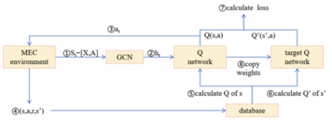
Figure 2. Algorithm framework diagram
The main algorithmic framework is shown in Figure 2. Initially, the agent acquires the current state through its interaction with the environment, which is represented by a feature attribute matrix of nodes (including CPU resources, storage resources, and the bandwidth and latency of adjacent links) and an adjacency matrix. This state is input into the GCN, where it undergoes message aggregation and updates, resulting in the output vector ht. Based on this vector information, the agent makes a decision regarding the action to take, which is then applied to the environment to receive a reward and determine the next state. The experience replay buffer stores the state, action, reward, and next state. During offline training, the DQN extracts multiple sets of experience values from this buffer to compute the Q-values and loss values, subsequently updating the weight parameters. The detailed process is described as follows:
Step 1: The agent observes the MEC network environment to obtain the current state.
Step 2: The current state is input into the GCN, which outputs the state encoding after graph convolution.
Step 3: The Q-values are calculated based on the current state, leading to the selection of the optimal action.
Step 4: After executing the SFC orchestration task, a tuple $\left(\mathrm{s}, \mathrm{a}, \mathrm{r}, \mathrm{s}^{\prime}\right)$ consisting of the current state, action, reward, and next state is generated and stored in the database, enabling continuous updates to the Deep Reinforcement Learning model.
Step 5: The Q-values are computed for both the current state and the next state.
Step 6: The predicted Q-values and current Q-values are determined.
Step 7: The loss function is calculated, and the network weights are updated.
Step 8: The Q network weights are copied to the Target Q network.
4.3 Model training process
In each time slot t, user arrivals are modeled using a Poisson process. Given that the state in graph structure cannot be directly input into a fully connected neural network, it is necessary to encode the state into a real-valued vector. To achieve this, we leverage the Graph Convolutional Network architecture outlined in study [23], which operates through the following steps.
By exploiting the intrinsic features of each node within the graph, we utilize a Graph Convolutional Network to effectively aggregate the neighborhood information associated with each node. In this case, we employ a multi-layer GCN with a standard hierarchical propagation rule:
$\mathrm{H}^{(1+1)}=\sigma\left(\widetilde{\mathrm{D}}^{-\frac{1}{2}} \widetilde{\mathrm{A}} \widetilde{\mathrm{D}}^{-\frac{1}{2}} \mathrm{H}^{(1)} \mathrm{W}^{(\mathrm{l})}\right)$ (21)
Here, $\widetilde{A}=A+I$ represents the adjacency matrix of the undirected graph with added self-connections, and I denotes the identity matrix. $\widetilde{\mathrm{D}}$ is the degree matrix, $\mathrm{H}^{(1)}$ is the input feature representation of the nodes at layer 1-th, $\mathrm{H}^{(0)}=\mathrm{X} . \mathrm{W}^{(1)}$ represents the weight matrix for layer 1-th, and $\sigma(\cdot)$ is the activation function.
The complexity of the given GCN formula can be analyzed as follows: First, computing $\widetilde{A}=A+$ Irequires $O\left(N^2\right)$ for a dense graph, where $N=\left|N^s\right|$ is the number of nodes. Calculating $\widetilde{\mathrm{D}}^{-\frac{1}{2}}$ involves $\mathrm{O}(\mathrm{N})$ since it only requires summing the rows of the adjacency matrix and taking the square root. Multiplying $\widetilde{\mathrm{D}}^{-\frac{1}{2}} \widetilde{\mathrm{A}}^{-\frac{1}{2}}$ has a complexity of $\mathrm{O}\left(\mathrm{N}^2\right)$ for dense graphs. For the feature matrix operations, $\mathrm{H}^{(1)} \mathrm{W}^{(1)}$ takes $\mathrm{O}\left(\mathrm{N} \cdot \mathrm{F}^{(1)} \cdot \mathrm{F}^{(1+1)}\right)$, where $\mathrm{F}^{(1)}=\mathrm{F}^{(1+1)}=2 *\left|\mathrm{~N}^s\right|+5$ in this study and multiplying the normalized adjacency matrix with the feature matrix requires $\mathrm{O}\left(\mathrm{N}^2 \cdot \mathrm{~F}^{(1)}\right)$ for dense graphs. Overall, the total complexity is $\mathrm{O}\left(\mathrm{N}^2+\mathrm{N}^2 \cdot \mathrm{~F}^{(1)}+\mathrm{N} \cdot\right.$ $\left.\mathrm{F}^{(1)} \cdot \mathrm{F}^{(1+1)}\right)$ for dense graphs.
During the training phase, an $\varepsilon$-greedy strategy is employed to select random actions with a defined probability, facilitating exploration of the environment. After an action is executed, the state, next state, action, and reward, are recorded in the database. Once the database accumulates a sufficient number of entries to meet the minimum batch size, a batch of data is sampled to train the Q-network after each exploratory step. The loss function applied during the training process is expressed in Eq. (22):
$\mathrm{L}(\theta)=\mathrm{E}\left[\mathrm{r}+\gamma \max _{\mathrm{a}^{\prime}} \mathrm{Q}\left(\mathrm{s}^{\prime}, \mathrm{a}^{\prime} ; \theta_{\mathrm{T}}\right)-\mathrm{Q}(\mathrm{s}, \mathrm{a} ; \theta)\right]$ (22)
In this context, $\theta$ and $\theta_{\mathrm{T}}$ represent the Q network and the target Q network, respectively. The first part of the loss function $r+\gamma \max _{\mathrm{a}}$ $\mathrm{Q}\left(s^{\prime}, \mathrm{a}^{\prime} ; \theta_{\mathrm{T}}\right)$ signifies the target Q value predicted by the target network, $\max _a$, $Q\left(s^{\prime}, a^{\prime} ; \theta_T\right)$ corresponds to the Q value for action $\mathrm{a}^{\prime}$ derived from the next state $s^{\prime}$ is used as input to the target network, with $\gamma$ representing the discount factor. The $\mathrm{Q}(\mathrm{s}, \mathrm{a} ; \theta)$ corresponds to the Q value computed by the current Q network. Consequently, the loss function captures the model's estimation error. A smaller loss indicates improved model performance. The Q-network weights are updated through the gradient descent algorithm.
$\begin{gathered}\theta^{\prime}=\theta+\alpha\left[r+\gamma \max _{\mathrm{a}^{\prime}} \mathrm{Q}\left(\mathrm{s}^{\prime}, \mathrm{a}^{\prime} ; \theta_{\mathrm{T}})\right.-\mathrm{Q}(\mathrm{s}, \mathrm{a} ; \theta)\right] \mathrm{Q}(\mathrm{s}, \mathrm{a} ; \theta)\end{gathered}$ (23)
In Eq. (23), θ and θ′ represent the parameters of the Q network before and after the update, respectively, while α denotes the learning rate.
The pseudocode for the training process is outlined in Algorithm 1 as follows:
|
Algorithm 1: Training Process of GCN-DQN |
|
1: Initialize the target Q network $\mathrm{Q}\left(\mathrm{s}^{\prime}, \mathrm{a}^{\prime} ; \theta_{\mathrm{T}}\right)$ and Q network $Q(s, a ; \theta)$ with random weights 2: Initialize experience replay memory D to capacity N 3: for each episode do 4: Initialize the environment 5: for each time slot t do 6: the arrival of n SFCs following a Poisson process 7: for each SFC do 8: obtain the current state s of the environment 9: Select action a according to an $\varepsilon$-greedy policy based on $Q(s, a ; \theta)$ 10: Perform action a, then observe the resulting reward r and the subsequent state s' 11 Record the transition (s, a, r, s') in D 12: end for 13: Randomly sample a minibatch of transitions from D 14: For each transition (s, a, r, s') in minibatch do 15: Set y = $\mathrm{r}+\gamma \max _\mathrm{a}^{\prime} \mathrm{Q}\left(\mathrm{s}^{\prime}, \mathrm{a}^{\prime} ; \theta_{\mathrm{T}}\right)$ 16: Update $Q(s, a ; \theta)$ by minimizing the loss: $L(\theta)=E[y-Q(s, a ; \theta)]$ 17: Update the target Q network $\mathrm{Q}\left(\mathrm{s}^{\prime}, \mathrm{a}^{\prime} ; \theta_{\mathrm{T}}\right)$ with weights $\theta_{\mathrm{T}} \leftarrow \theta$ 18: end for 19: end for 20: end for |
5.1 Simulation environment and design
This study uses the open source network function virtualization resource allocation simulation software, SFCSim [24], as a simulation tool. SFCSim enables dynamic SFC orchestration simulations in mobile scenarios. The simulation environment utilizes the Cernnet network topology, as illustrated in Figure 3. This network consists of 23 edges and 21 nodes.
Figure 3. Cernnet network topology
The simulation parameters are specified in Table 1. In the network, the number of CPU cores in the edge computing nodes follows a uniform distribution U(100 cores,300 cores). The bandwidth of the links between nodes is 2.5 Gbps, and the propagation delay of the links ranges from 0.5 ms to 1.6 ms. The network supports eight types of virtual network functions. The resource coefficient for processing traffic per Mbps is uniformly distributed between 0.025 and 0.05 cores, while traffic proportion coefficients for each type of VNF follow a uniform distribution U(0.8,1.2). Service function chain arrivals in different time slots are assumed to follow a Poisson distribution, with traffic demands ranging from 20 Mbps to 40 Mbps and latency requirements between 8 ms and 10 ms. The traffic needs to pass through between 2 and 5 network functions.
Table 1. Simulation parameters
|
|
Parameters |
Value |
|
NFVI |
Node Resources |
U(100cores,300cores) |
|
Link Bandwidth |
2.5Gbps |
|
|
Transmission Delay |
0.5-1.6ms |
|
|
VNF |
Type |
8 |
|
Traffic scaling factor |
U(0.8,1.2) |
|
|
Resource Coefficient |
0.025-0.05cores/Mbps |
|
|
SFC |
Traffic Demand |
20-40Mbps |
|
Latency Requirement |
8-10ms |
|
|
Number of Required Network Functions |
2-5 |
|
|
Lifetime |
1-3 time slot |
The Q network within the agent is built with two GCN layers and two fully connected layers. The size of the state space corresponds to the input layer, while the size of the action space corresponds to the output layer. During training, the neural network’s learning rate is set to 0.001, and the discount factor is set to 0.95. For the learning rate, 0.001 serves as a baseline value. In our experiments, we adopted the Adam optimizer, which dynamically computes the effective learning rate for each update based on gradient momentum and normalization operations, enabling more effective learning. Regarding the discount factor, we prioritized long-term rewards, which led us to select a relatively large value of 0.95.
The first comparative algorithm is the Static Edge Chain Allocation (SECA) algorithm [25], which is designed for SFC orchestration in MEC environments for mobile users. The core idea of SECA is to sequentially treat all nodes along the shortest path from the destination node to the source node as candidate nodes, deploying the SFC's network functions on these candidate nodes in order. If the resources of the current candidate node are insufficient, the deployment is moved to the next candidate node. This algorithm utilizes the shortest path to guide traffic.
The second comparative algorithm employs DQN exclusively to select a traffic steering path from k shortest paths. The node deployment strategy aligns with that of the SECA algorithm. This algorithm maintains consistency and comparability in node placement within the network structure by adhering to the same deployment strategy for VNFs as SECA. It intelligently selects paths solely through DQN, optimizing network traffic allocation, enhancing transmission efficiency, and reducing congestion.
5.2 Simulation results
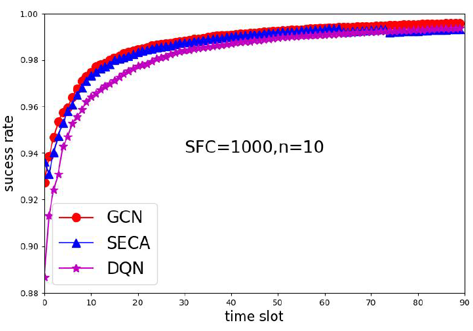
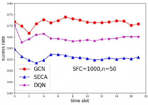
Initially, we assessed the performance of the GCN-DQN in the topology depicted in Figure 3, which was also utilized during the training phase. The deployment success rates of various algorithms over time are presented in Figures 4-6, corresponding to SFC arrival rates of 10, 20, and 50, respectively. The total number of SFCs simulated is 1000, indicating that the simulation concludes after 1000 SFCs have appeared in the network. At time slot t=0, there are already 40 SFCs in the network, and their deployment status is included in the overall deployment success rate. From the figures, it is evident that as time progresses, the deployment success rate initially increases and then stabilizes. This is due to the fact that the 40 existing SFCs have not yet reached the end of their service time. As time increases, the deployment success rate gradually rises and eventually stabilizes, particularly at lower arrival rates. However, when the arrival rate is set to 50, this value approaches that of the initial 40 SFCs, resulting in minimal changes in the deployment success rate over time.
Figure 4. SFC deployment success rate at an arrival rate of 10
Figure 5. SFC deployment success rate at an arrival rate of 20
Figure 6. SFC deployment success rate at an arrival rate of 50
Figure 7 shows the deployment success rates of different algorithms under varying arrival rates. The figure clearly demonstrates that the GCN-based algorithm consistently outperforms both the DQN-only and SECA algorithms. This improvement can be attributed to the GCN's ability to model the network, allowing for a better understanding of the relationships between network nodes and leading to more effective deployment decisions.
Figure 7. Average deployment success rate of algorithms under different arrival rates of the topology during training
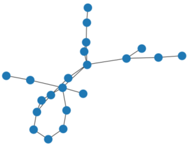
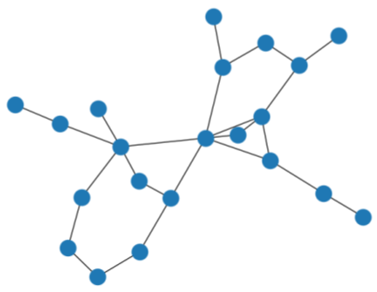
Subsequently, we extended our experiments by conducting simulations in a network environment whose topology deviates from the one used during the training phase, as depicted in Figure 8. Unlike the structured topology presented in Figure 3, the node connections in this new topology exhibit distinct patterns and arrangements, reflecting a more complex and dynamic network layout. This deliberate variation in topology aims to assess the robustness and adaptability of the GCN-DQN algorithm under diverse conditions, ensuring its generalizability beyond the specific topologies it was initially trained on.
Figure 8. Network topology
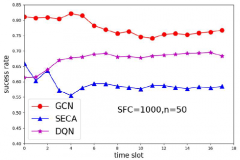
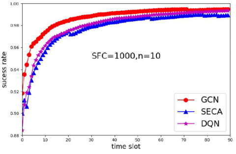
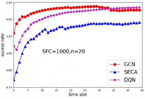
In this particular network topology, the simulation results are comprehensively illustrated in Figures 9-12. These figures present a detailed comparison of the deployment success rates under various conditions. The findings suggest that, even when confronted with previously unseen network topologies, our proposed algorithm consistently maintains a high level of performance, achieving a satisfactory deployment success rate. This robustness in diverse topological scenarios highlights the generalizability and adaptability of the algorithm. Furthermore, as shown in Figure 9, when comparing the deployment success rates, the algorithm utilizing only the DQN approach reveals a significant disparity, particularly at lower SFC arrival rates. This suggests that our proposed algorithm, which integrates additional optimization strategies, effectively outperforms the DQN-only approach, ensuring more reliable and efficient traffic steering decisions under challenging conditions, especially when traffic volumes are relatively low.
Figure 9. SFC deployment success rate at an arrival rate of 10
Figure 10. SFC deployment success rate at an arrival rate of 20
Figure 11. SFC deployment success rate at an arrival rate of 50
Figure 12. Average deployment success rate of algorithms under different arrival rates of non-trained topologies
To enhance the persuasiveness of our experimental results, we also trained the DQN-only algorithm on the network topology shown in Figure 8 and then tested its SFC deployment success rate in that network. We compared this with the GCN-DQN algorithm, which had not been trained on that topology. We similarly evaluated the SFC deployment success rates under different arrival rates and calculated the averages, as presented in Figure 13. From the figure, we can see that the deployment success rate of the DQN algorithm improved compared to Figure 12. However, at arrival rates of 10 and 20, the deployment success rate still fell short of that of the GCN-DQN algorithm. At an arrival rate of 50, the deployment success rate slightly exceeded that of the GCN-DQN algorithm. Additionally, we conducted similar tests in other topologies, yielding consistent results. Therefore, we can conclude that the GCN-DQN algorithm demonstrates good generalization capability. However, the current topology requires the number of nodes to be consistent with the number of nodes in the topology used during training.
Figure 13. Average deployment success rate of algorithms under different arrival rates after DQN retraining
We have summarized the comparison of the GCN-DQN algorithm with other existing methods, particularly its key performance in optimizing SFC traffic steering paths. The experimental results reveal that the GCN-DQN approach exhibits notable advantages across different network topologies and load conditions, achieving a higher SFC request acceptance rate than the traditional DQN algorithm, all while satisfying QoS constraints. The introduction of GCN enables the algorithm to better capture network topology, improving decision-making efficiency and scalability. Moreover, GCN-DQN exhibits strong generalization capabilities, effectively performing SFC orchestration in unseen network topologies. These results fully demonstrate the innovation and practicality of the GCN-DQN algorithm compared to other methods in MEC environments.
This paper investigates the dynamic orchestration of Service Function Chains in MEC environments across different network topologies. To address this issue, we conduct an in-depth analysis of network latency and user services in MEC environments. To enhance the overall revenue of network services while meeting user latency requirements, we model the dynamic orchestration of SFCs in MEC environments as a 0-1 ILP model. Subsequently, we propose an intelligent orchestration strategy for SFCs based on graph neural networks and deep reinforcement learning. GCN-DQN intelligently decides on traffic steering paths by perceiving network topology states and user service demands through GCN and DQN. Extensive experimental simulations demonstrate that GCN-DQN can better perceive the relationships within network topologies compared to existing algorithms, leading to superior decision-making and robust generalization capabilities.
In future work, we plan to evaluate the performance of the proposed model in large-scale network topologies to further validate its robustness and applicability. To address the memory and GPU limitations commonly encountered during GCN training, we will incorporate the GraphSAGE [26] method to enable efficient node sampling and aggregation. This approach will allow the graph model to scale effectively for handling large graph-structured data, thereby enhancing the practicality of the GCN-based SFC orchestration method in extensive MEC environments.
Additionally, we will explore strategies for SFC readjustment to better adapt to dynamic changes in user demands and network conditions. This involves developing mechanisms for real-time updates to service chain deployments while minimizing their impact on network operations and optimizing resource utilization.
We also aim to tackle potential challenges related to scalability and real-world application of the framework by proposing corresponding solutions. Specifically, we will analyze and optimize the algorithm's computational complexity to improve its efficiency for real-time operations in large-scale networks. To address challenges arising from the heterogeneity of MEC infrastructures, we will explore how to adapt to diverse hardware capabilities and develop a modular design to enhance compatibility. Furthermore, we plan to leverage distributed computing techniques to offload computational burdens, thereby mitigating resource constraints and improving the overall performance of the framework.
Through these efforts, we aim to further enhance the adaptability and scalability of the GCN-DQN framework and provide effective solutions for its broader application in diverse and dynamically evolving MEC environments.
[1] Hantouti, H., Benamar, N., Taleb, T. (2020). Service function chaining in 5G & beyond networks: Challenges and open research issues. IEEE Network, 34(4): 320-327. https://doi.org/10.1109/MNET.001.1900554
[2] Arulkumaran, K., Deisenroth, M. P., Brundage, M., Bharath, A.A. (2017). Deep reinforcement learning: A brief survey. IEEE Signal Processing Magazine, 34(6): 26-38. https://doi.org/10.1109/MSP.2017.2743240
[3] Zhou, J., Cui, G., Hu, S., Zhang, Z., Yang, C., Liu, Z., Sun, M. (2020). Graph neural networks: A review of methods and applications. AI Open, 1: 57-81. https://doi.org/10.1016/j.aiopen.2021.01.001
[4] Aurrecoechea, C., Campbell, A.T., Hauw, L. (1998). A survey of QoS architectures. Multimedia Systems, 6: 138-151. https://doi.org/10.1007/s005300050083
[5] Sonkoly, B., Czentye, J., Szalay, M., Németh, B., Toka, L. (2021). Survey on placement methods in the edge and beyond. IEEE Communications Surveys & Tutorials, 23(4): 2590-2629. https://doi.org/10.1109/COMST.2021.3101460
[6] Chen, Y.T., Liao, W. (2019). Mobility-aware service function chaining in 5G wireless networks with mobile edge computing. In ICC 2019-2019 IEEE International Conference on Communications (ICC), Shanghai, China, pp. 1-6. https://doi.org/10.1109/ICC.2019.8761306
[7] Taleb, T., Ksentini, A., Frangoudis, P.A. (2016). Follow-me cloud: When cloud services follow mobile users. IEEE Transactions on Cloud Computing, 7(2): 369-382. https://doi.org/10.1109/TCC.2016.2525987
[8] Mouradian, C., Kianpisheh, S., Abu-Lebdeh, M., Ebrahimnezhad, F., Jahromi, N.T., Glitho, R.H. (2019). Application component placement in NFV-based hybrid cloud/fog systems with mobile fog nodes. IEEE Journal on Selected Areas in Communications, 37(5): 1130-1143. https://doi.org/10.1109/JSAC.2019.2906790
[9] Mosayebi, A., Pozveh, A.J. (2020). Heuristic based algorithm for SFC allocation in 5G experience applications. In 2020 6th Iranian Conference on Signal Processing and Intelligent Systems (ICSPIS), Mashhad, Iran, pp. 1-6. https://doi.org/10.1109/ICSPIS51611.2020.9349535
[10] Shokouhifar, M. (2021). FH-ACO: Fuzzy heuristic-based ant colony optimization for joint virtual network function placement and routing. Applied Soft Computing, 107: 107401. https://doi.org/10.1016/j.asoc.2021.107401
[11] Fu, X., Yu, F.R., Wang, J., Qi, Q., Liao, J. (2019). Service function chain embedding for NFV-enabled IoT based on deep reinforcement learning. IEEE Communications Magazine, 57(11): 102-108. https://doi.org/10.1109/MCOM.001.1900097
[12] Li, G., Feng, B., Zhou, H., Zhang, Y., Sood, K., Yu, S. (2020). Adaptive service function chaining mappings in 5G using deep Q-learning. Computer Communications, 152: 305-315. https://doi.org/10.1016/j.comcom.2020.01.035
[13] Liu, Y., Lu, H., Li, X., Zhang, Y., Xi, L., Zhao, D. (2020). Dynamic service function chain orchestration for NFV/MEC-enabled IoT networks: A deep reinforcement learning approach. IEEE Internet of Things Journal, 8(9): 7450-7465. https://doi.org/10.1109/JIOT.2020.3038793
[14] Wang, L., Mao, W., Zhao, J., Xu, Y. (2021). DDQP: A double deep Q-learning approach to online fault-tolerant SFC placement. IEEE Transactions on Network and Service Management, 18(1): 118-132. https://doi.org/10.1109/TNSM.2021.3049298
[15] Sun, P., Lan, J., Li, J., Guo, Z., Hu, Y. (2020). Combining deep reinforcement learning with graph neural networks for optimal VNF placement. IEEE Communications Letters, 25(1): 176-180. https://doi.org/10.1109/LCOMM.2020.3025298
[16] Heo, D., Lange, S., Kim, H.G., Choi, H. (2020). Graph neural network based service function chaining for automatic network control. In 2020 21st Asia-Pacific Network Operations and Management Symposium (APNOMS), Daegu, Korea (South), pp. 7-12. https://doi.org/10.23919/APNOMS50412.2020.9236954
[17] Qi, S., Li, S., Lin, S., Saidi, M.Y., Chen, K. (2021). Energy-efficient VNF deployment for graph-structured SFC based on graph neural network and constrained deep reinforcement learning. In 2021 22nd Asia-Pacific Network Operations and Management Symposium (APNOMS), Tainan, Taiwan, pp. 348-353. https://doi.org/10.23919/APNOMS52696.2021.9562610
[18] Xiao, D., Zhang, J.A., Liu, X., Qu, Y., Ni, W., Liu, R.P. (2023). A two-stage GCN-based deep reinforcement learning framework for SFC embedding in multi-datacenter networks. IEEE Transactions on Network and Service Management, 20(4): 4297-4312. https://doi.org/10.1109/TNSM.2023.3284293
[19] Kuo, T.W., Liou, B.H., Lin, K.C.J., Tsai, M.J. (2018). Deploying chains of virtual network functions: On the relation between link and server usage. IEEE/ACM Transactions on Networking, 26(4): 1562-1576. https://doi.org/10.1109/TNET.2018.2842798
[20] Gouareb, R., Friderikos, V., Aghvami, A.H. (2018). Virtual network functions routing and placement for edge cloud latency minimization. IEEE Journal on Selected Areas in Communications, 36(10): 2346-2357. https://doi.org/10.1109/JSAC.2018.2869955
[21] Wang, L., Lu, Z., Wen, X., Knopp, R., Gupta, R. (2016). Joint optimization of service function chaining and resource allocation in network function virtualization. IEEE Access, 4: 8084-8094. https://doi.org/10.1109/ACCESS.2016.2629278
[22] Pei, J., Hong, P., Xue, K., Li, D. (2018). Efficiently embedding service function chains with dynamic virtual network function placement in geo-distributed cloud system. IEEE Transactions on Parallel and Distributed Systems, 30(10): 2179-2192. https://doi.org/10.1109/TPDS.2018.2880992
[23] Bai, Y., Ding, H., Bian, S., Chen, T., Sun, Y., Wang, W. (2019). SimGNN. In Proceedings of the Twelfth ACM International Conference on Web Search and Data Mining, USA. https://doi.org/10.1145/3289600.3290967
[24] Xu, L., Hu, H., Liu, Y. (2023). SFCSim: A network function virtualization resource allocation simulation platform. Cluster Computing, 26(1): 423-436. https://doi.org/10.1007/s10586-022-03670-8
[25] Zheng, G., Tsiopoulos, A., Friderikos, V. (2019). Dynamic VNF chains placement for mobile IoT applications. In 2019 IEEE Global Communications Conference (GLOBECOM), Waikoloa, HI, USA, pp. 1-6. https://doi.org/10.1109/GLOBECOM38437.2019.9014166
[26] Huang, K., Chen, C. (2024). Subgraph generation applied in GraphSAGE deal with imbalanced node classification. Soft Computing, 28(17-18): 10727-10740. https://doi.org/10.1007/s00500-024-09797-7