Time Series Clustering of GARCH (1,1) Model Using Modified Piccolo Distance

The model of primary focus is the GARCH (1,1) model, which combines the corrected mean return at a point in time and its variance. Research indicates that the GARCH (1,1) model is highly effective for accurately modeling time series data and is the most popular model adopted for time series [22]. This is done by parsimony, which effectively reduces the number of parameters in the ARCH model and generalizes them to other parameters [23]. This section will explore the theoretical basis of the distance between two GARCH (1,1) models.

2.1 GARCH (1,1) model

The GARCH (1,1) model is widely recognized as one of the foremost models for analyzing various time series data [20]. This model adheres to the principle of parsimony by effectively reducing the number of parameters present in ARCH models and generalizing them into alternative parameters [22]. According to Bollerslev [23], the GARCH (1,1) model is considered the most suitable for characterizing financial data. Its simplicity, involving only two parameters, facilitates the calculation of the distance between two GARCH (1,1) models, thereby enhancing its utility in practical applications.

It is known that $\varepsilon_t=r_t-\mu_t$ the mean corrected log return, $\varepsilon_t$ adheres to the GARCH (1,1) model [21] if

$\varepsilon_t=v_t \sigma_t$    (1)

with

$\sigma_t^2=\gamma+\alpha_1 \varepsilon_{t-1}^2+\beta_1 \sigma_1 \varepsilon_{t-1}^2$    (2)

where, $v_t \sim \operatorname{IID}(0,1), \gamma>0, \alpha_1 \geq 0, \beta_1 \geq 0$ and $\left(\alpha_1+\right.$ $\left.\beta_1\right)<1$. Assumed $E\left(\varepsilon_t \mid F_{t-1}\right)=0, \operatorname{Var}\left(\varepsilon_t \mid F_{t-1}\right)=$ $E\left(\varepsilon_t^2 \mid F_{t-1}\right)=\sigma_t^2$.

2.2 Parameter estimation of GARCH (1,1) model

Parameter estimation of $\gamma, \alpha_1$ and $\beta_1$ in the GARCH (1,1) model requires modeling the regression such that

$y_t=\tau_0+\tau_1 y_{t-1}+\varepsilon_t, t=1, \ldots, T$    (3)

with

$\varepsilon_t=v_t \sigma_t=v_t \sqrt{h_t}, h_t=\gamma+\alpha_1 \varepsilon_{t-1}^2+\beta_1 h_{t-1}$    (4)

The parameter vector $\tilde{\theta}$ is expressed as

$\tilde{\theta}=\left(\tau_0, \tau_1, \gamma, \alpha_1, \beta_1\right)^{\prime}=\left(\tilde{\tau}^{\prime}, \tilde{\delta}^{\prime}\right)$

with

$\tilde{\tau}=\left[\begin{array}{l}\tau_0 \\ \tau_1\end{array}\right], \tilde{\delta}=\left[\begin{array}{c}\gamma \\ \alpha_1 \\ \beta_1\end{array}\right]$

In general, Eq. (3) is an AR (1) model with $\tau_0$ as a constant and $\tau_1$ autoregressive coefficients, while the GARCH (1,1) model is according to Eq. (2), which is rewritten in Eq. (4). For this reason, because the GARCH (1,1) model is used, the parameters estimated according to Eq. (4) are $\gamma, \alpha_1$ and $\beta_1$. To estimate the parameters of $\gamma, \alpha_1$ and $\beta_1$ begins by finding the likelihood function on:

$f\left(\varepsilon_t \mid F_{t-1}\right)=\frac{1}{\sqrt{2 \pi h_t}} e^{-\frac{1 \varepsilon_t^2}{2 h_t}}$    (5)

The likelihood function for the $t$ observation and sample size expressed with $T$ is denoted by $L_t$, then:

$L_t=-\frac{1}{2} \ln 2 \pi-\frac{1}{2} \ln h_t-\frac{1}{2} \frac{\varepsilon_t^2}{h_t}$     (6)

Furthermore, it is derived from $\tilde{\delta}$, obtained:

$\frac{\partial L_t}{\partial \tilde{\delta}}=\frac{1}{2 h_t} \frac{\partial h_t}{\partial \tilde{\delta}}\left(\frac{\varepsilon_t^2}{h_t^2}-1\right)=\frac{1}{2}\left(\frac{1}{h_t}\right) \tilde{b}_t v_t$    (7)

The iteration form is derived from the modified Newton-Raphson method as follows:

$\tilde{\delta}_{i+1}=\tilde{\delta}_i-\left[\sum_{t=1}^T v_t^2\left(\frac{1}{2} \frac{\tilde{b}_t}{h_t}\right)\left(\frac{1}{2} \frac{\tilde{b}_t}{h_t}\right)^{\prime}\right]^{-1} \sum_{t=1}^T \frac{1}{2}\left(\frac{1}{h_t}\right) \tilde{b}_t v_t$      (8)

with 

$\tilde{b}_t=\frac{\partial h_t}{\partial \tilde{\delta}} \frac{\varepsilon_t^2}{h_t^2}, v_t=\frac{\partial h_t}{\partial \tilde{\delta}}$

2.3 Distance between two GARCH (1,1) models

The distance between two GARCH (1,1) models is calculated based on an extension of the ARMA (1,1) model distance proposed by Piccolo [13]. The time series model with $t=1,2, \cdots, T$ is as follows:

Model 1: $y_{1, t}=\mu_1+\varepsilon_{1, t}$

Model 2: $y_{2, t}=\mu_2+\varepsilon_{2, t}$

where, $\varepsilon_{1, t}$ and $\varepsilon_{2, t}$ are errors with zero mean and time-varying variance. It is assumed that the variances $h_{1, t}$ and $h_{2, t}$ adhere to two distinct and independent GARCH (1,1) structures, as in Eq. (4),

$\begin{aligned} & \sigma_{1, t}^2=h_{1, t}=\gamma_1+\alpha_1 \varepsilon_{1, t-1}^2+\beta_1, h_{1, t-1} \\ & \sigma_{2, t}^2=h_{2, t}=\gamma_2+\alpha_2 \varepsilon_{2, t-1}^2+\beta_2, h_{2, t-1}\end{aligned}$

with $\gamma_i>0,0<\alpha_i<1,0<\beta_i<1,\left(\alpha_i+\beta_i\right)<1(i=1,2)$. Further, $V_t$ be a zero-mean ARMA invertible process and F is a class of invertible ARMA processes. It is known that if $V_t \in F$, then, there exists a constant $\pi_i$ such as

$\sum_{j=1}^{\infty}\left|\pi_j\right|<\infty$

and

$V_t=\sum_{j=1}^{\infty} \pi_j V_{t-j}+\varepsilon_t$, with $\varepsilon_t \sim W N\left(0, \sigma^2\right)$

The distance between two processes $V_{1 t}, V_{2 t} \in F$ is defined as stated by Piccolo and then called Piccolo distance [13].

$\begin{gathered}d^2\left(V_{1 t}, V_{2 t}\right)=\sum_{j=1}^{\infty}\left(\pi_{1 j}-\pi_{2 j}\right)^2 \\ d=\left[\sum_{j=1}^{\infty}\left(\pi_{1 j}-\pi_{2 j}\right)^2\right]^{\frac{1}{2}}\end{gathered}$            (9)

with $\pi_{1 j}$ and $\pi_{2 j}$ are the coefficients of the two AR processes. From Eq. (9), the distance of two GARCH (1,1) models is as follows:

$\begin{gathered}d=\left(\sum_{j=0}^{\infty}\left(\alpha_1 \beta_1^j-\alpha_2 \beta_2^j\right)^2\right)^{\frac{1}{2}} \\ d=\left(\frac{\alpha_1^2}{1-\beta_1^2}+\frac{\alpha_2^2}{1-\beta_2^2}-\frac{2 \alpha_1 \alpha_2}{1-\beta_1 \beta_2}\right)^{\frac{1}{2}}\end{gathered}$      (10)

2.3.1 Modified Piccolo distance

Modified Piccolo distance is the new distance that is different from the Piccolo distance in the GARCH model (see Eq. (10)) developed by Otranto [24]. The background of the modified Piccolo distance is based on the Manhattan distance, where the calculation method for the distance space applies the concept of absolute difference. The squared distance is generally the most used distance metric, as in Eq. (9). Still, it has some disadvantages compared to the absolute distance, which is sensitive to outliers. Since the difference of the data is squared, if there is extreme data in one dimension, the overall value of the squared distance can increase significantly, so the outlier value will greatly affect the result of the distance calculation. This is one of the motivations to modify the Piccolo distance using absolute values. Then, the distance between the two processes $V_{1 t}, V_{2 t} \in F$ is defined as

$d=\sum_{j=1}^{\infty}\left|\pi_{1 j}-\pi_{2 j}\right|$        (11)

with $\pi_{1 j}$ and $\pi_{2 j}$ are the coefficients of the two AR processes, like the Piccolo distance for the GARCH model by Otranto [24]. From Eq. (11), the distance between two GARCH (1,1) models, which is a modification of the Piccolo distance, is shown below:

$\begin{gathered}d=\sum_{j=1}^{\infty}\left|\alpha_1 \beta_1^{j-1}-\alpha_2 \beta_2^{j-1}\right| \\ =\sum_{j=0}^{\infty}\left|\alpha_1 \beta_1^j-\alpha_2 \beta_2^j\right|=\left|\alpha_1 \sum_{j=0}^{\infty} \beta_1^j-\alpha_2 \sum_{j=0}^{\infty} \beta_2^j\right| \\ =\left|\alpha_1\left(\beta_1^0+\beta_1^1+\beta_1^2+\cdots\right)-\alpha_2\left(\beta_2^0+\beta_2^1+\beta_2^2+\cdots\right)\right| \\ =\left|\frac{\alpha_1}{1-\beta_1}-\frac{\alpha_2}{1-\beta_2}\right|\end{gathered}$             (12)

2.3.2 Distance measure by Caiado

Two-time series each fit the GARCH (1,1) model, with $\pi_1=\left(\alpha_1, \beta_1\right)$ and $\pi_2=\left(\alpha_2, \beta_2\right)$ as the parameter estimation vectors. Furthermore, $S_1$ and $S_2$ are estimates of the variance-covariance matrix, respectively. Caiado and Crato [29] defined the distance between volatilities of time series data as

$d=\left(\pi_1-\pi_2\right)^{\prime} S^{-1}\left(\pi_1-\pi_2\right)$    (13)

where, $S=S_1+S_2$. This distance captures all the stochastic structure of a process's conditional variance and offers a solution for comparing time series data of unequal lengths [29].

2.3.3 Maharaj distance

Maharaj et al. [14, 30] proposed a hypothesis test that has practical applications in evaluating whether there is a significant difference between two-time series. This test is designed to assess whether the generation processes of the two-time series differ significantly. The corresponding test statistic is defined as follows:

$d=\sqrt{T}\left(\pi_1-\pi_2\right)^{\prime} S^{-1}\left(\pi_1-\pi_2\right)$     (14)

with $T$ is the length of the series, $\pi_1=\left(\alpha_1, \beta_1\right)$ and $\pi_2=\left(\alpha_2, \beta_2\right)$ as the parameter estimation vectors. $S=\sigma_1^2 R_1^{-1}+\sigma_2^2 R_2^{-1}$, where $\sigma_1^2$ and $\sigma_2^2$ are the variances of the white noise processes for each series, $R_1$ and $R_2$ the samples covariance matrices of both series.

The null hypothesis $\left(H_0\right)$ is rejected at the $\alpha$ significance level when the statistic $d>\chi^2(k)$, where $\chi^2(k)$ denotes the $(1-\alpha)$ th quantile of the chi-square distribution with $k$ degrees of freedom. If the null hypothesis is rejected, it indicates that the series $y_{1, t}$ and $y_{2, t}$ generating processes are significantly different [14].

2.3.4 Distance cosine

Cosine distance is a quantitative measure of dissimilarity between two vectors and is calculated as the complement of the cosine similarity value. Cosine similarity assesses the degree of similarity between two vectors by evaluating the cosine of the angle formed between them. The Euclidean dot product formula can determine this cosine value for two non-zero vectors.

$\pi_1 \cdot \pi_2=\left\|\pi_1\right\|\left\|\pi_2\right\| \cos (\theta)$

with $\pi_1=\left(\alpha_1, \beta_1\right)$ and $\pi_2=\left(\alpha_2, \beta_2\right)$ as the parameter estimation vectors. The cosine similarity, $\cos (\theta)$ is represented using a dot product given two $n$-dimensional vectors, $\pi_1$ and $\pi_2$.

$\begin{gathered}\text { cosine similarity }=\cos (\theta)=\frac{\pi_1 \cdot \pi_2}{\left\|\pi_1\right\|\left\|\pi_2\right\|} \\ \qquad \cos (\theta)=\frac{\sum_{i=1}^n \pi_{1 i} \pi_{2 i}}{\sqrt{\sum_{i=1}^n \pi_{1 i}^2} \cdot \sqrt{\sum_{i=1}^n \pi_{2 i}^2}}\end{gathered}$     (15)

where, $\pi_{1 i}$ and $\pi_{2 i}$ are the $i$ th components of vectors $\pi_1$ and $\pi_2$, respectively. The cosine distance between two vectors $\pi_1$ and $\pi_2$ is defined as:

$\text {cosine distance} \left(\pi_1, \pi_2\right)=1-\cos (\theta)$   (16)

with $\cos (\theta)$ is the cosine similarity calculated according to Eq. (15).

4.1 Simulation

The simulated data consists of 15 time series clustered into 3 clusters. Each cluster consists of 5 time series with 100 points in each time series. The following provides a detailed description of each cluster.

Cluster 1. GARCH (1,1) Model, with

$h_t=0.005+0.1 \varepsilon_{t-1}^2+0.1 h_{t-1}$

Cluster 2. GARCH (1,1) Model, with

$h_t=0.1 \varepsilon_{t-1}^2+0.8 h_{t-1}$

Cluster 3. GARCH (1,1) Model, with

$h_t=-0.005+0.9 \varepsilon_{t-1}^2+0.01 h_{t-1}$

The steps of the clustering process include:

1. Generate time series using the GARCH (1,1) model with the conditions described in the simulation data above. Repeat for each model (Cluster 1, 2, and 3) with 5 time series each.
2. Calculate the distance between time series using different distances based on the estimated GARCH (1,1) parameters according to Eqs. (10)-(16).
3. Implementation of clustering algorithm

1. Hierarchical Clustering

1. Use complete linkage as the linkage method according to Eq. (17).
2. Input the distance between time series calculated in Step 2 into the hierarchical clustering algorithm.

2. K-means Clustering

1. Initialize the initial centroid using 3 random time series from the dataset (since the number of clusters is 3).
2. Assign each time series to the cluster with the smallest distance from the centroid.
3. Update the centroid to show the average of the estimated parameters of each cluster.
4. Repeat the above steps until it converges.

4. Evaluate the validity of clustering results using the C-index validity measure.

Figure 1 shows the average line of each cluster. Table 1 shows the results of 5 distance measures with hierarchical complete linkage and K-means clustering algorithms. The complete linkage method based on Eq. (17) minimizes the variance between clusters in hierarchical clustering. As for K-means, the initial centroid initialization process is randomly selected from the existing dataset. Furthermore, the C-index is used to measure the validity of the cluster.

2.1.png

Figure 1. Plot of each cluster

Table 1. Clustering with simulation data

Algorithm	Distance	C-Index
Hierarchical	Piccolo	0.578118
	Modified Piccolo	0.578118
	Caiado	0.450013
	Maharaj	0.450013
	Cosine	0.450013
K-means	Piccolo	0.578118
	Modified Piccolo	0.455615
	Caiado	0.007818
	Maharaj	0.001686
	Cosine	0.001686

Table 1 shows that the best-performing hierarchical clustering with small c-index values is obtained using Caiado, Maharaj, and cosine distances. Then, in K-means clustering, Maharaj and cosine distance gave the best performance. However, when compared to the Piccolo distance, the modified Piccolo distance produces a smaller c-index for K-means clustering.

4.2 Stock data analysis

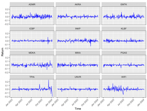
The case study used data from twelve stocks listed on the Indonesia Stock Exchange using daily closing prices taken from Yahoo Finance. These stocks include PT Adaro Minerals Indonesia Tbk (ADMR), PT AKR Corporindo Tbk (AKRA), PT Elang Mahkota Teknologi Tbk (EMTK), PT Indofood CBP Sukses Makmur Tbk (ICBP), PT Indah Kiat Pulp and Paper Tbk (INKP), PT Kalbe Farma Tbk (KLBF), PT Merdeka Copper Gold Tbk (MDKA), PT Mitra Keluarga Karyasehat Tbk (MIKA), State Gas Company (PGAS), PT Chandra Asri Pacific Tbk, PT Unilever Indonesia Tbk (UNVR), and PT Solusi Sinergi Digital Tbk from January 3^rd, 2023 until January 9^th, 2024. The first step is to calculate the return, and then each stock return is estimated using the GARCH (1,1) model according to Eq. (4).

2.2.png

Table 3. Recapitulation of cluster members for hierarchical clustering with Piccolo and modified Piccolo distance

Table 4. Recapitulation of cluster members for K-means clustering with Caiado and cosine distance

Figure 2 shows the return plot for each stock. Each stock shows different volatility. It can be seen that TPIA and WIFI stocks show higher volatility spikes compared to others. Table 2 shows the results of 5 distance measures with hierarchical complete linkage and K-means clustering algorithms. Similarly to what was done with the simulated data, in hierarchical clustering, the complete linkage method based on Eq. (17) minimizes the variance between clusters. For K-means, the initial centroid initialization process is randomly selected from the existing data set. Next, the C-index measures the validity of the cluster.

In Table 2, the hierarchical clustering algorithm with the distance that gives the best performance is the small c-index value achieved in Piccolo and modified Piccolo distance. In K-means clustering, Caiado and cosine distance gave the best performance. Furthermore, Table 3 shows the clusters formed for hierarchical clustering with Maharaj, Caiado, and cosine distance, and Table 4 shows K-means clustering with Caiado and cosine distance.

Table 3 shows that two clusters with the same cluster members are obtained for each of the Piccolo and modified Piccolo distances. K-means clustering can be seen in Table 4, where two clusters with the same cluster members are also obtained using Caiado and cosine distances.

The clustering results based on GARCH (1,1) models allow investors to identify asset groups with similar volatility patterns. From the clustering results, two clusters with different volatility patterns are obtained. Stocks in one cluster tend to have similar volatility parameters, providing a framework for selecting assets from different clusters. TPIA and WIFI stocks that show higher volatility (also shown in Figure 2) are in the same group. The results are expected to reduce the risk in portfolio selection. For example, investors can combine stocks from high-volatility clusters with stocks from low-volatility clusters to create a more balanced portfolio. Information from the clusters can also be used to determine the optimal weight of assets in the portfolio. Stocks in lower-risk clusters can be given more weight for conservative investors, while stocks from high-volatility clusters can be included in smaller proportions to increase profit opportunities. Furthermore, the clusters formed can be updated regularly as market volatility patterns change. This helps investors adjust the portfolio to dynamic market conditions, such as increased volatility during periods of economic uncertainty. The ability to cluster assets based on volatility patterns aims to provide analytical tools for investors and portfolio managers. Therefore, these clustering results bridge theoretical models of volatility and practical applications in investment decision-making.