Yassin Masrar*![]() | Mohamed Ettaouil
| Mohamed Ettaouil
© 2025 The authors. This article is published by IIETA and is licensed under the CC BY 4.0 license (http://creativecommons.org/licenses/by/4.0/).
OPEN ACCESS
In this work, a finite element numerical model for hyperelastic axisymmetric and plane strains is described. The variational formulation used is an intermediate formulation between mixed method and penalty method. The choice of the proposed method makes it possible to avoid the high computational cost in the mixed method, and the reduced integration which can generate a divergence of the numerical solution in the penalty method. A good agreement between the numerical solution and the exact analytical solution is proved for the two deformation models, with adoption of convergence criterion based simultaneously on vectorial norms of displacement and hydrostatic pressure fields and vectorial norms of their increments. Then, a detailed study on the convergence of the numerical solution is carried out by considering the influence of the theoretical approximation of hydrostatic pressure on this convergence, in order to determine the incompressibility parameter for good convergence. This study show that the choice of the value attributed to the incompressibility parameter must be chosen in the order of 0.0001 but not necessarily smaller, so as not to slow down the convergence of the numerical solution. The numerical model of axisymmetric strain is also applied in a design study of a cylindrical laminated elastomeric bearing.
axisymmetric strains, elastomeric bearing, finite element analysis, hyperelasticity, nonlinear strains, numerical convergence, plane strains
Numerical processing by finite elements has particularly proven its effectiveness in the analysis of geometrically nonlinear structures since the work of Turner et al. [1]. The first works dealing with large strains of incompressible hyperelastic materials were reported by Becker [2] and Oden [3]. Becker numerically studied the finite plane strains of a rubber sheet subjected to kinematic boundary conditions in the work of Turner et al. [1]. This problem of finite plane strains was taken up by Oden [3], where he established the nonlinear stiffness equations. The functional used is that of the potential energy into which the incompressibility constraint was introduced by the method of the Lagrange multipliers. This was the procedure suggested by Truesdell and Toupin [4] for general variational under constraints and used for the study of infinitesimal deformations by Herrmann [5]. However, the numerical resolution of the equations for incompressible nonlinear elasticity would not be approached until the beginning of the 1970s, and comparisons of solutions by finite elements with analytical solutions were proposed. First was the mixed method or Lagrange multiplier method with two fields (displacement and hydrostatic pressure), used by many authors for the study of rubber strains, in particular Scharnhorst and Pian [6] in an axisymmetric strain study and Batra [7] in a plane strain study. However, the difficulties encountered in the implementation of these methods using conventional computer codes led to the development of other methods, such as the penalty method, where the numerical resolution is only carried out in the displacement field. However, in the majority of cases, these methods call for the reduced integration technique and stiffness matrix calculation in the finite element method, which generally results in problems with the convergence of the numerical solution. This convergence problem in relation to these methods was raised very early by Oden [8], Zdunek and Bercovier [9], and even nowadays it is not sufficiently treated in the literature.
Among the studies dealing with the convergence of the numerical solution in the field carried out during the last two decades, Stein and Sagar [10] proposed examining quadratic convergence of finite element analysis for hyperelastic material under finite strain via ABAQUS, as well as classifying the rates of convergence for iterative solutions in regular cases. Baroli et al. [11] presented a discontinuous Galerkin method applied to incompressible nonlinear elasticity, in a total Lagrangian formulation, with appropriate application of the interior penalty stabilization technique. They asserted that the discrete formulation proposed for the linearized problem was convergent, the stability of the numerical scheme was addressed in detail, and optimal error estimates for deformations and pressure in different norms were derived, confirmed by several numerical experiments in two and three spatial dimensions. Karoui et al. [12] presented a convergence study of the numerical solution within the framework of the Extended Finite Element Method (XFEM), applied to the study of cracked hyperelastic materials, in order to overcome the limitations of the classical finite element method when it was used for such cases. Mei et al. [13] presented a new method to transform the discretised governing equations to improve the rate of convergence of numerical schemes in Newton's solvers, in order to solve highly nonlinear elasticity problems, even when steps of extremely large loads are applied. They confirmed that their approach was simple to implement and could be integrated into any existing finite element code. Farrell et al. [14] adapted the three-field formulation for nearly incompressible hyperelasticity introduced by Chavan et al. [15] for construct mixed finite element schemes, and they proposed a new augmented Lagrangian preconditioner that improved the convergence properties of iterative solvers and compared them favorably to classical two-field schemes. Barnafi et al. [16] addressed the implementation and performance of the inexact Newton–Krylov and quasi-Newton algorithm methods in solving nonlinear elasticity equations, and they were interested in the convergence of these methods. They suggested that the quasi-Newton method should be preferred for compressible mechanics, whereas the inexact Newton–Krylov method should be preferred for incompressible problems. They claimed that these methods show adequate performance and provide significant speed over the standard Newton–Krylov method. Hong et al. [17] proposed and analyzed an abstract stabilized mixed finite element framework that can be applied to nonlinear incompressible elasticity problems. They considered applying an abstract stabilized framework in which any mixed finite element method that satisfies certain conditions can be modified so that it is stable and optimally convergent. Kadapa and Hossain [18] proposed a two-field mixed formulation that they considered to be a simplified and efficient alternative to the three-field displacement–pressure–Jacobian formulation used for hyperelastic materials. They compared their formulation with that programmed in ABAQUS, particularly with regard to improving the convergence rate of Newton–Raphson iterations, and noted the usefulness of introducing an artificial numerical constant to overcome the difficulties of the solver. They concluded that their formulation was more effective and did not pose the same problems as Abaqus in this area.
Fradet [19] raises the issue of convergence of numerical solution in a resolution by Newton’s method of rubber fracture problem in some applications, and proposes the use of a model called “cohesive zone model” to overcome the numerical difficulties due to the nonlinearity of the problem coupled with the singularity at the crack tip. Prabhune and Suresh [20] consider that an important requirement in the standard finite element method (FEM) is that all elements of the underlying mesh must be tangle-free, i.e., the Jacobian must be positive in each element, they introduce a variational formulation which leads to a local modification of the tangent stiffness matrix associated with the entangled elements, with the aim of generalizing with the field of the nonlinear deformations compressible and incompressible, the method known as “Isoparametric tangled finite elements method (i-TFEM) proposed recently to solve the problems of linear elasticity. They claim that the (i-TFEM) leads to an optimal convergence of the numerical solution even for severely tangled meshes, and that it reduces to the standard (FEM) method for tangle-free meshes. Mountris et al. [21] consider an explicit method for the analysis of finite deformations of hyperelastic materials called the total Lagrangian Fragile Points Method (FPM). This method was used to derive an explicit total Lagrangian algorithm for the finite deformation and does not make use of the domain mesh like the finite element method. They claim that the proposed method has been evaluated, comparing it to FEM in several case studies, considering both extension and compression of a hyperelastic material, and that FPM has been shown to maintain a good accuracy even for large deformations where the FEM did not converge. Luo et al. [22] are interested in tests to determine the mechanical properties of hyperelastic membranes, such as the test called “planar equibiaxial tension test” with the aim of designing an effective equibiaxial tension test bench to meet the requirements of experimental precision. They use ABAQUS finite element software to simulate equibiaxial plane tension methods and study the impact of tightening mode on test accuracy and global strain uniformity. They also conclude that the four-parameter Ogden model allows an accurate description of the membrane material. Canales et al. [23] propose an optimization method called evolutionary strategy to characterize anisotropic hyperelastic materials, using the anisotropic hyperelastic model of Holzapfel-Gasser-Ogden, and numerical simulations by the finite element method.
About recent work on the mathematical modeling of elastomeric bearings, Kalfas et al. [24] pointed out that the issue of damage caused by the yielding of reinforcing steel shims in seismic isolation elastomeric bearings has received relatively limited attention in the literature. They aimed to explore, using the finite element method, how the characteristics of steel reinforcement influence the behavior of rubber bearings subjected to combined axial load, shear displacement, and rotation. Similarly, Mazza and Mazza [25] emphasized that the design of elastomeric bearings, which are used to protect structures from earthquake damage, is typically based on nonlinear models that primarily account for the effects of shear and compressive loads. They propose to examine the impact of tensile loads, generated by severe earthquakes, on the performance of bearings and the superstructure. Han and Che [26] conducted an experimental and numerical study to determine the shear modulus of an offshore elastomeric support. They aim to establish the optimal analysis conditions for a numerical simulation with a nonlinear model of ANSYS software for elastomeric material. The main objective is that these numerical results are in good agreement with the experimental results. Leblouba [27] studied the stability of Elastomeric bearings (EB) and lead-rubber bearings (LRB) used in bridge structures to reduce vehicle vibrations, wind loads, and earthquakes. It proposes two nonlinear mathematical models adapted to these components, to adequately account for the interaction between the horizontal and vertical loads and their effect on the bearing’s performance. He affirms that comparisons with experimental tests demonstrated that the two developed mathematical models could accurately replicate the behavior of seismic isolators, and can readily be incorporated into structural analysis software such as Open Sees. Premnath and Gopi [28] claim that the vibration in ships causes structural fatigue, damage to electrical and mechanical devices, excessive level of noise and discomfort to the passengers and crews. They study vibration reduction in marine machinery using elastomeric bearings. The numerical study was carried out using the ANSYS software and validated with experimental tests. By comparing the calculated loss factor of different elastomeric materials, for determining the best damping material, they concluded that the styrene-butadiene rubber (SBR) and the poly-butadiene rubber (PBR) can be used for high-frequency damping applications.
This paper presents intermediate variational formulation, whose numerical resolution is carried out only with the displacement field, but without recourse to reduced integration and while keeping the field of hydrostatic pressure present at each iteration of convergence. This formulation is used for axisymmetric and plane strains analysis for hyperelastic hollow cylinder subjected to uniform internal pressure. The problem of convergence of the numerical solution is addressed, considering the influence of the hydrostatic pressure approximation on the convergence of the proposed method. The epsilon factor (Eq. (7)), suitable for good convergence of the method is determined for the two strain models.
2.1 Variational formulation
The finite element numerical processing of hyperelastic media requires the development of computational software that can satisfactorily predict the behavior of the medium under study. In most applications, the hyperelastic material is highly stressed, and its behavior becomes nonlinear. The nonlinearities are both materials, due to the constitutive law of the material, and geometric, due to the large deformations, to which is added the incompressibility constraint.
►Constitutive law, stresses, and strains:
In the study of the equilibrium problem of the medium, with total Lagrangian formulation [29], the second tensor of Piola-Kirchoff $S^{i j}$ for the definition of stresses is used. The Green strain tensor $E_{ij}$ for the definition of the strains is used. The behavior law of the elastomer is then given by the following relation:
$C^{i j j d}=\frac{\partial S^{i j}}{\partial E_{k l}}$ (1)
where, Cijkl represents the elasticity tensor coefficients, comprising a symmetric tensor of order 4.
►Piola-Kirchoff second tensor Sij:
Similarly, knowledge of the elastic potential W of the elastomer makes it possible to determine the second Piola-Kirchoff stress tensor, by the following relationship:
$S^{i j}=\frac{\partial W}{\partial E_{i j}}$ (2)
►Elastic potential W(I1,I2):
In the literature, it is found that various expressions to approach the elastic potential W according to the invariants I1, I2, and I3 of the deformation, such as the two-coefficient model of Mooney-Rivlin, given by
$W=C_1\left(I_1-3\right)+C_2\left(I_2-3\right)$ (3)
where, C1 and C2 denotes the material constants
►Modified elastic potential W(I1,I2,I3):
In the numerical processing, the incompressibility of the elastomeric material is taken into account by considering a modified elastic potential W* as follows:
$W^*\left(I_1, I_2, I_3\right)=W\left(I_1, I_2\right)+p \cdot G\left(I_3\right)$ (4)
where, p is hydrostatic pressure and G(I3) is a function of the invariant I3, which can be approximated by the following logarithmic function [30]:
$G\left(I_3\right)=0.5 \ln \left(I_3\right)$ (5)
►Modified potential energy functional π(u,p):
The equilibrium formulation of the hyperelastic material is then given by the stationarity of the modified potential energy functional, as follows:
$\begin{aligned} & \pi(u, p)=\int_{V_0}\left(W\left(I_1, I_2\right)+p \cdot G\left(I_3\right)\right) d V -\int_{V_0} \rho_0 f^i u_i d V-\int_{\Gamma_0}{ }^0 t^i u_i d \Gamma\end{aligned}$ (6)
where, V0 is the undeformed volume and Γ0 is its charged boundary surface; fi and 0ti are the volume load and areal load vector, respectively; and ρ0 is density.
The stationarity of π(u,p) makes it possible to provide a system of nonlinear equations that can be solved directly by the Newton–Raphson method. However, the mixed resolution is often delicate and difficult to implement, so preference may be given to carrying out resolution in the displacement field only, by considering an approximation for the pressure field at each finite element.
►Intermediate variational formulation:
In this work, the following approximation for the hydrostatic pressure field on a given finite element e is presented:
$p^e=\frac{1}{\varepsilon \cdot V_0^e} \cdot \int_{V_0^e} G\left(I_3\right) d V$ (7)
where, $V_0^e$ denotes the undeformed volume of the element, and ε denotes the incompressibility parameter of order 10-4.
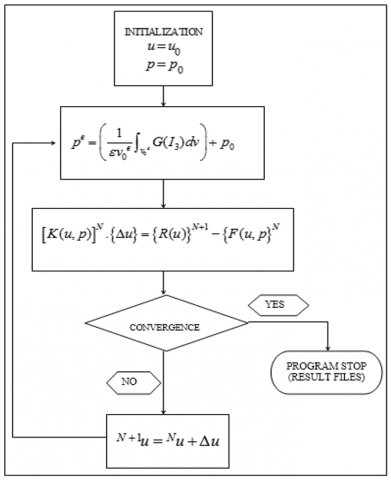
Figure 1. Software resolution flowchart
This approximation of the hydrostatic pressure is omnipresent in all iteration of convergence, as shown in the flowchart in Figure 1. What makes that one is not really in the presence of a method of resolution with only one field, but in an intermediate method between mixed method of resolution with two fields and method of resolution with only one field.
►Convergence criterion:
The convergence criterion adopted in the method is a mixed criterion on the two fields, displacements and hydrostatic pressure, as follows:
$\frac{\|\Delta \vec{u}\|}{\|\vec{u}\|} \leq 10^{-4}$ and $\frac{\|\Delta p\|}{\|p\|} \leq 10^{-4}$ (8)
2.2 Incremental equilibrium equation in incompressible nonlinear elasticity
The incremental equilibrium equation obtained from the formulation developed in section 2.1, and as shown in the software resolution flowchart of Figure 1, is given in the following matrix form expression by:
$[K(u, p)]^N \cdot\{\Delta u\}=\{R(u)\}^{N+1}-\{F(u, p)\}^N$ (9)
where, [K(u, p)]N is the stiffness matrix known at iteration N, {Δu} is the displacement increment vector calculated at iteration N+1, {F(u, p)}N is the internal load vector known at iteration N (previous deformed configuration (CN)), and {R(u)}N+1 is the external load vector introduced at iteration N+1 (deformed configuration (CN+1)).
Eq. (9) is also written with the detailed form of the stiffness matrix [K(u, p)]N as follows:
$\left(\left[K_L\right]^N+\left[K_{N L}\right]^N+\left[K_{I N C}\right]^N\right) \cdot\{\Delta u\}=\{R\}^{N+1}-\{F\}^N$ (10)
where, [KL] denotes the stiffness matrix of large deformations, [KNL] denotes the stiffness matrix of initial stresses, and [KINC] denotes the stiffness matrix representing the incompressibility effects in the deformed configuration (CN). The computation of the global stiffness matrix [K] thus requires the computation of the three preceding stiffness’s matrices.
2.2.1 Elementary stiffness matrix [KL]e
The elementary stiffness matrix associated with the stiffness matrix of large deformations [KL] is given by:
$\left[K_L\right]^e=\int_{V_0^e}\left[B_i\right]^T[C]\left[B_j\right] d V$ (11)
where, [C] denotes the elasticity matrix, and [Bi] denotes the displacements-linear strains transformation matrix.
►Transformation matrix [Bi]:
The displacements-linear strains transformation matrix [Bi] is given by:
$\left[B_i\right]=\left[\frac{\partial \varepsilon_{p q}}{\partial u_{\alpha_i}}\right]$ (12)
where, εpq denotes the physical components of the Green strain tensor, and $u_{\alpha_i}$ denotes the components of the elementary nodal displacements vector {δ} defined by
$\{\delta\}=\left\langle u_{\alpha_i}\right\rangle(\alpha, i) \in\{p, q, r\} \times\{1,2, \ldots, I\}$ (13)
with I the number of total element nodes, and (p,q,r) is the coordinate system used.
►Elasticity matrix [C]:
The elasticity matrix [C] is given by:
$[C]=\left[C^{i j k l}\right]=\left[\frac{\partial^2 W^*}{\partial \varepsilon_{i j} \partial \varepsilon_{k l}}\right]$ (14)
with
$C^{i j k l}=\frac{\partial^2 W^*}{\partial \varepsilon_{i j} \partial \varepsilon_{k l}}=\frac{\partial^2 W}{\partial \varepsilon_{i j} \partial \varepsilon_{k l}}+p \frac{\partial^2 G}{\partial \varepsilon_{i j} \partial \varepsilon_{k l}}$ (15)
where, W* is the modified elastic potential defined in section 2.1 (Eq. (4)).
2.2.2 Elementary stiffness matrix [KNL]e
The elementary stiffness matrix associated with the stiffness matrix of initial stresses [KNL] is given by:
$\left[K_{N L}\right]^e=\int_{V_0^e}\left[L_i\right]^T[S]\left[L_j\right] d V$ (16)
►Transformation matrix [Li]:
[Li] In the Eq. (16) is the following transformation matrix:
$\{\partial u\}=\left[L_i\right]\{\delta\}$ (17)
In which {δ} denotes the vector previously defined by Eq. (13), and {∂u} is the vector defined by:
$\langle\partial u\rangle=\left\langle\frac{\partial u_\alpha}{\partial \beta}\right\rangle(\alpha, \beta) \in\{p, q, r\} \times\{p, q, r\}$ (18)
where, uα denote the component of the displacement field vector, and (p,q,r) is the coordinate system used.
For example, the explicit form of {∂u} and {δ} vectors, in the cylindrical coordinate system, in axisymmetric strains problem, are given by:
$\left\{\begin{array}{lllll}\langle\partial u\rangle=\left\langle\begin{array}{llll}\frac{\partial u_r}{\partial r} & \frac{\partial u_r}{r} & \frac{\partial u_z}{\partial r} & \frac{\partial u_r}{\partial z}& \frac{\partial u_z}{\partial z}\end{array}\right\rangle \\ \langle\delta\rangle=\left\langle\begin{array}{lll}u_{r_i} & u_{z_i}\end{array}\right\rangle \quad i=1,2, \ldots, I\end{array}\right.$ (19)
In the Cartesian coordinate system, in-plane strain problems, are given by:
$\left\{\begin{array}{llll}\langle\partial u\rangle=\left\langle\begin{array}{llll}\frac{\partial u_x}{\partial x} & \frac{\partial u_y}{\partial x} & \frac{\partial u_x}{\partial y} & \frac{\partial u_y}{\partial y}\end{array}\right\rangle \\ \langle\delta\rangle=\left\langle\begin{array}{lll}u_{x_i} & u_{y_i}\end{array}\right\rangle \quad i=1,2, \ldots, I\end{array}\right.$ (20)
►Initial stresses matrix [S]:
The matrix [S] in Eq. (16), called initial stresses matrix, verifies the following equation:
$[A(u)]^T \cdot\{S\}=[S] \cdot\{\partial u\}$ (21)
where, {S} denotes the Piola-Kirchoff stresses vector defined in cylindrical coordinate, for axisymmetric strains problem, by:
$\langle S\rangle=\left\langle\begin{array}{llll}S^{r r} & S^{\theta \theta} & S^{z z} & S^{r z}\end{array}\right\rangle$ (22)
Defined in Cartesian coordinates for a plane strains problem in the plane (x, y) by:
$\langle S\rangle=\left\langle S^{x x} \quad S^{y y} \quad S^{x y}\right\rangle$ (23)
The [A(u)] matrix in Eq. (21) necessary for the [S] matrix determination is defined by the expression:
$\left\{\eta_{i j}\right\}=\frac{1}{2}[A(u)] \cdot\{\partial u\}$ (24)
with ηij the nonlinear part, in the decomposition of the strain tensor into a linear and a nonlinear part as follows:
$\varepsilon_{i j}=e_{i j}+\eta_{i j}$ (25)
2.2.3 Elementary stiffness matrix [KINC]e
The expression of elementary stiffness matrix associated with [KINC] is given by:
$\left[K_{N V C}\right]^e=\int_{V_0^e}\left[B_i\right]^T[G]\left[B_j\right] d V$ (26)
In which [G] denotes the incompressibility effects matrix.
For the determination of the elementary stiffness matrix [KINC]e representing the incompressibility effects in the deformed configuration (CN), displacements - linear strains transformation matrix [Bi] and the incompressibility effects matrix [G] as seen in the Eq. (26) must be first calculated. Matrix [Bi] was previously defined in section 1 above, and the matrix [G] is defined in the following point.
►Incompressibility effects matrix [G]:
This matrix is defined by the following equation:
$[G]=\left[G^{i j kl}\right]=\left\{\partial G^{i j}\right\}\left\langle\partial G^{kl}\right\rangle$ (27)
where the vector $\left\langle\partial G^{k l}\right\rangle$ in cylindrical coordinate, for axisymmetric strains problem is given by:
$\left\langle\partial G^{kl}\right\rangle=\left\langle\begin{array}{llll}\frac{\partial G}{\partial \varepsilon_{r r}} & \frac{\partial G}{\partial \varepsilon_{\theta \theta}} & \frac{\partial G}{\partial \varepsilon_{z z}} & \frac{\partial G}{\partial\left(2 \varepsilon_{r z}\right)}\end{array}\right\rangle$ (28)
In Cartesian coordinates, a plane strains problem is given by:
$\left\langle\partial G^{kl}\right\rangle=\left\langle\frac{\partial G}{\partial \varepsilon_{x x}} \frac{\partial G}{\partial \varepsilon_{y y}} \frac{\partial G}{\partial\left(2 \varepsilon_{x y}\right)}\right\rangle$ (29)
[G] is a symmetrical square matrix of order 4 in axisymmetric strains problem and order 3 in plane strains problem, similar to [C] (Eq. (14)).
2.3 Computational software in large strain
The resolution flowchart of the computational software in large strain developed in this work is presented in Figure 1.
The program has been validated by considering nonlinear elasticity problems with known exact analytical solutions such as the problem of the hyperelastic hollow cylinder subjected to uniform internal pressure studied in section 3.1.
3.1 Numerical solution in plane and axisymmetric strains for hyperelastic cylinder
In this section, the numerical model presented in section 2 is applied to the study of plane and axisymmetric nonlinear strains in the problem of an infinite hyperelastic hollow cylinder subjected to uniform internal pressure. The cylinder has an internal radius Ri of 6 in (152.4 mm) and an external radius Re of 8 in (203.2 mm), and the applied pressure pi is 30.438 psi (0.21 N/mm2). The Mooney–Rivlin behavior law is considered for the hyperelastic material (elastomer), with C1=37.66psi (0.26 N/mm2) and C2=23.30psi (0.161 N/mm2).
The exact mathematical solution of this problem is given by Green and Zerna [31] as follows:
$\left\{\begin{array}{l}p_i=\left(C_1+C_2\right)\left[\begin{array}{l}\ln \frac{R_i^2+b}{R_e^2+b}-2 \ln \frac{R_i}{R_e} \\ +b \frac{R_e^2-R_i^2}{\left(R_e^2+b\right)\left(R_i^2+b\right)}\end{array}\right] \\ b=2 R_i \tilde{u}_r+\tilde{u}_r^2\end{array}\right.$ (30)
$\left\{\begin{array}{l}p=-p_i-2 C_2 \\ -2\left(C_1+C_2\right)\left[\ln \frac{r}{R_i}+\frac{b}{2}\left(\frac{1}{r^2}-\frac{1}{R_i^2}\right)-\ln \frac{R}{R_i}+\frac{R^2}{r^2}\right] \\ r=R+u_r\end{array}\right.$ (31)
$\left\{\begin{array}{l}
\sigma^{rr}=p+2 C_2+2\left(C_1+C_2\right) \frac{R^2}{r^2} \\
\sigma^{\theta \theta}=p+2 C_2+2\left(C_1+C_2\right) \frac{r^2}{R^2}
\end{array}\right.$ (32)
where, ur denotes radial displacement, $\tilde{u}_r$ denotes radial displacement for any point on the internal surface of the cylinder, and p denotes hydrostatic pressure; σrr and σθθ are the radial and tangential Cauchy stresses, respectively; and r and R are the radius of a point in the deformed and undeformed configuration of the body, respectively.
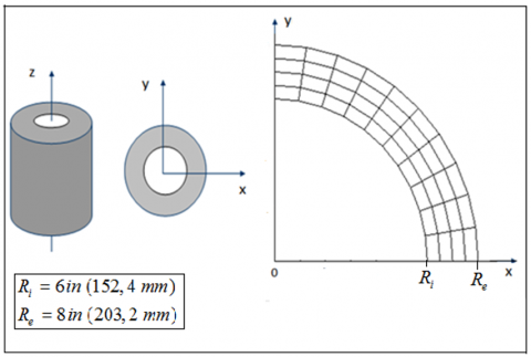
Figure 2. Plane finite element mesh, of elastomeric cylinder modeled with 40 four-node finite elements
Figure 3. Axisymmetric finite element mesh, of elastomeric cylinder modeled with 10 four-node finite elements
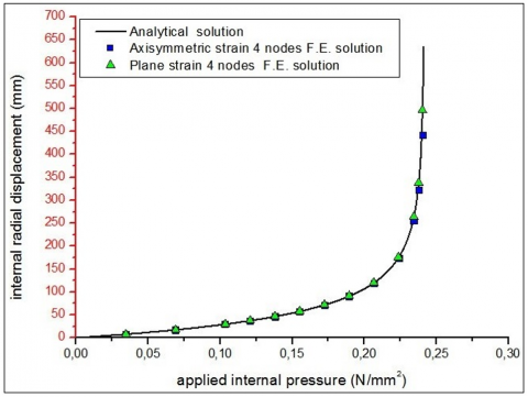
Figure 4. Internal displacement evolution for Mooney-Rivlin model
Figure 2 shows the finite element mesh considered for the studied cylinder within the framework of the plane strain assumption. Due to the symmetrical conditions (geometric and boundary conditions), a quarter of the cylinder plane section orthogonal to the axis of revolution $O \vec{Z}$ is modelled with 40 four-node finite elements (Figure 2). In the same way, Figure 3 shows the finite element mesh considered for the cylinder within the framework of the assumption of axisymmetric strain. In this case, a band of low height h taken in an axial section (θ=cte) of the cylinder is modelled with 10 axisymmetric four-node finite elements (Figure 3). Since the plane strain and axisymmetric strain assumptions are checked at the same time for this problem of the hollow cylinder, the results of the axisymmetric strain model are presented together with those obtained for the plane strain model.
The results obtained with the constitutive Mooney–Rivlin law for the two strain models considered reveal good agreement between the numerical and analytical solutions, as shown in Figure 4. The tests revealed that the numerical solution obtained with the axisymmetric strain model is more precise than that obtained with the plane strain model for fairly high applied pressures approaching the limit of pi=35psi(0.241 N/mm2). Indeed, for the Mooney-Rivlin model, there is an applied limit pressure, beyond which the numerical solution diverges.
Figure 5. Hydrostatic pressure distribution in the cylinder
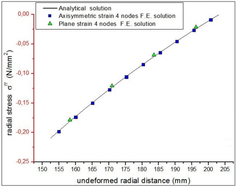
Figure 6. Radial stress distribution in the cylinder
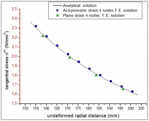
Figure 7. Tangential stress distribution in the cylinder
The programming of the analytical solution Eqs. (30)-(32) makes it possible to check that no imposed displacement, however large, will make it possible to obtain an imposed pressure higher than this value.
The curve of the function $p_i=f\left(u_{R_i}\right)$ therefore presents an asymptotic branch, in the vicinity to the left of the value pi=35psi(0.241 N/mm2) (see Figure 4). The hydrostatic pressure and stress field in the elastomeric material were studied for an applied pressure of pi=30.438psi(0.21 N/mm2).
Figure 5 shows the evolution of hydrostatic pressure in the elastomer, and Figures 6 and 7 show this evolution for radial stress σrr and tangential stress σθθ, respectively. They show good agreement of the numerical solution with the analytical solution for the two strain models.
3.2 Study of the numerical solution convergence in the two strain models
A study of the numerical solution convergence was also carried out, looking for the impact of factor ε in Eq. (7) on the convergence error of this solution [32].
The study shows that the value ε=10-4 is acceptable for the axisymmetric strain model, where the errors remain low, even for pressure close to the limit value pi=35psi(0.241316 N/mm2). This value of ε can also be adopted for the plane strain model up to an applied pressure close to pi=33.500psi(0.230974 N/mm2).
As an example, in this model, with an applied pressure of pi=34.985psi(0.241213 N/mm2) the error is 4.063 in (103.200 mm) for the internal numerical displacement of the cylinder, while in the axisymmetric model, it is only 0.447 in (11.354 mm).
Table 1 gives the convergence error of the numerical solution for the internal displacement of the cylinder according to the internal pressure applied for the two models of plane and axisymmetric strain. It shows that under high pressure, the convergence error becomes important, and in this case, it will be necessary to find a good value that should be assigned to coefficient ε in the numerical study for an optimal convergence error. The study also reveals that the axisymmetric strain model is more precise than the plane strain model, which is acceptable in terms of design, and although there appears to be more convergence iterations in the axisymmetric model (see Table 1), this model requires much less computation time to reach the solution. Indeed, for the problem of the hollow cylinder in axisymmetric mesh (10 four-node finite elements), the number of equations to solve for each iteration of convergence in the system is only 22, whereas for the plane strain mesh (40 four-node finite elements) the system solution comprises 100 equations.
Table 2 gives the values adopted for the plane strain model for convergence coefficient ε for applied pressure between 33,500 psi (0.231 N/mm2) and 35.00 psi (0.241 N/mm2) in order to obtain a numerical solution with an optimal convergence error.
Table 1. Convergence error of the numerical solution, in axisymmetric strains and plane strains models
|
|
|
Plane Strains Model |
Axisymmetric Strains Model |
||||
|
Applied Pressure pi (N/mm2) |
Analytical Solution $\boldsymbol{u}_r^{a n}$ (mm) |
Numerical Solution $\boldsymbol{u}_r^{n u}$ (mm) |
CV Error with ε=10-4 |
Iter CV |
Numerical Solution $\boldsymbol{u}_r^{n u}$ (mm) |
CV Error with ε=10-4 |
Iter CV |
|
0.22429017 |
177.8 |
176.45126 |
1.34874 |
34 |
179.13604 |
1.33604 |
34 |
|
0.22774895 |
198.12 |
196.1134 |
2.0066 |
39 |
199.65924 |
1.53924 |
40 |
|
0.230815 |
222.25 |
219.14104 |
3.10896 |
46 |
223.94418 |
1.69418 |
47 |
|
0.23426689 |
262.001 |
256.54 |
5.461 |
59 |
264.2108 |
2.2098 |
62 |
|
0.23771189 |
335.28 |
322.326 |
12.954 |
88 |
338.3788 |
3.0988 |
96 |
|
0.24033698 |
490.22 |
442.595 |
47.625 |
165 |
496.6716 |
6.4516 |
211 |
|
0.24104665 |
622.3 |
519.0998 |
103.2002 |
232 |
633.6538 |
11.3538 |
361 |
|
0.24108799 |
635 |
525.272 |
109.728 |
238 |
647.192 |
12.192 |
378 |
|
0.24115 |
656.59 |
535.0764 |
121.5136 |
248 |
669.8742 |
13.2842 |
408 |
Table 2. Optimization of the convergence error in plane strains model
|
Applied Pressure pi(N/mm2) |
Analytical Solution $\boldsymbol{u}_r^{a n}$ (mm) |
Numerical Solution $\boldsymbol{u}_r^{n u}$ (mm) |
Adopted Factor ε |
Convergence Error $\Delta \boldsymbol{u}_r=\left|\boldsymbol{u}_r^{a n}-\boldsymbol{u}_r^{n u}\right|$ |
Iter CV |
|
0.230815 |
222.25 |
221.99346 |
3. D-04 |
0.25654 |
44 |
|
0.23095969 |
223.52 |
223.2914 |
3. D-04 |
0.2286 |
44 |
|
0.23426 |
262.001 |
261.366 |
4. D-04 |
0.635 |
57 |
|
0.237705 |
335.28 |
339.2932 |
9. D-04 |
4.0132 |
86 |
|
0.24104665 |
622.3 |
622.1984 |
(5.5). D-03 |
0.1016 |
234 |
|
0.24108799 |
635 |
634.3396 |
6. D-03 |
0.6604 |
241 |
|
0.24115 |
656.59 |
654.4564 |
7. D-03 |
2.1336 |
251 |
3.3 Modeling and computer-aided design (CAD) for cylindrical laminated elastomeric bearing
This section focuses on modeling and computer-aided design of elastomeric laminated cylindrical bearings, with the geometric formulation, using cylindrical coordinates, adapted to structures of revolution. The problem of bearings with a 3D parallelepiped structure, called plane bearings, has been treated in the previous study [33], with the geometric formulation, using Cartesian coordinates, adapted to this type of structure.
3.3.1 Local exploration of the stress field in elastomer layers
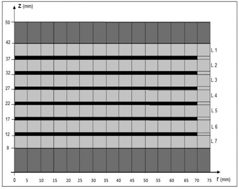
An industrial example consisting of the cylindrical laminated elastomeric bearing (CLEB) is shown in Figure 8.
The bearing, with a radius of 75 mm and height of 50 mm, has a rubber/metal composite structure, with seven layers of rubber interposed by six steel plates and two outside steel supports, and is subjected to an axial compressive load of 5000 daN. The thickness of the supports, elastomeric layers, and steel plates is 8, 4, and 1 mm, respectively. Table 3 summarizes the geometrical and Material parameters concerning the bearing studied.
Considering the structural, geometric, loading, and boundary conditions, the assumption of axisymmetric strain is retained. The boundary conditions here consist of fixing the lower support and assuming a uniform distribution of the pressure induced by the axial load on the upper support.
Table 3. Geometric and material parameters of the bearing
|
General Parameters of the Bearing |
|||||||
|
Diameter |
Height |
Applied axial force |
|||||
|
150 mm |
50 mm |
5000 daN |
|||||
|
Local parameters of the bearing |
|||||||
|
Geometric parameters |
Material parameters |
||||||
|
Externe Supports (Duralumin) |
Number |
2 |
Duralumin |
Young modulus |
E=7000 da N/mm2 |
||
|
Diameter |
150 mm |
Poisson's coefficient |
υ=0.34 |
||||
|
Thickness |
8 mm |
||||||
|
Elastomeric Layers (Rubber) |
Number |
7 |
Rubber |
Young modulus |
E=0.4140 da N/mm2 |
||
|
Diameter |
150 mm |
Poisson's coefficient |
υ=0.499999 |
||||
|
Thickness |
4 mm |
Behavior model (Mooney-Rivlin) |
C1=0.0552 da N/mm2 |
||||
|
C2=0.0138 da N/mm2 |
|||||||
|
Intermediary Plates (Steel) |
Number |
6 |
Steel |
Young modulus |
E=20000 da N/mm2 |
||
|
Diameter (CLEB-model1) |
140 mm |
Poisson's coefficient |
υ=0.3 |
||||
|
Diameter (CLEB-model2) |
150 mm |
||||||
|
Thickness |
1 mm |
||||||
Figure 8. Cylindrical laminated elastomeric bearing (CLEB-model 1)
Figure 9. Axisymmetric FE mesh of (CLEB-model 1) modeled by 225 four-node finite element
The choice of material model for the elastomer is typically determined by the user, who must experimentally identify the model's constants. In this study, the Mooney–Rivlin model was used with C1=0.0552 da N/mm2 and C2=0.0138 da N/mm2. The composite rubber/metal component is treated as a continuous domain, ensuring displacement continuity at the rubber–steel interfaces. For this to hold, perfect adhesion at the interfaces during the rubber injection process in manufacturing is required.
For the numerical analysis, axial section of the bearing in plane $(O, \vec{r}, \vec{z})$ of the cylindrical coordinate system $(O, r, \theta, z)$ was discretised with 225 four-node elements (Figure 9).
In addition, considering the linear elastic behavior of the external supports and intermediate plates, coarse meshing was adopted for these parts with a sufficient number of finite elements. The classical finite element of axisymmetric linear elasticity was used for these parts of the structure for elastomeric layers; considering the relative thinness of the layers and the precision of the formulation presented in this paper, one element was sufficient for modelling these layers in the z direction.
The results presented relate to the distribution of Cauchy's physical stresses on the seven elastomeric layers. Indeed, it is in these layers that the development of cracks is possible. This close investigations explore various areas of the laminated structure and obtains significant information for the design of the product, as well as the prediction of possible cracks.
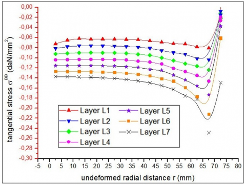
Figures 10-12 illustrate the distribution of unidirectional stresses σrr, σθθ, and σzz in the elastomeric layers as a function of the undeformed radial distance.
For each stress, the evolution is consistent across all layers, with maximum in absolute value in the vicinity of the edge of the bearing. Within the same elastomer layer, the evolution of the three unidirectional stresses is the same, with a slight difference for the σzz stress due to the compressive loading, which is in the direction of this stress. Indeed, the maximum unidirectional stresses are carried by this axial stress and are found on the lower layers, L6 and L7.
Figure 13 shows the evolution of shear stress as function of undeformed radial distance. The evolution of this stress is completely different from that of the other stresses. Its maximum value is located near the edge of the bearing on layer L6 and is significantly lower than the values obtained for the unidirectional stresses.
Figure 10. Radial stress distribution in elastomeric layers
Figure 11. Tangential stress distribution in elastomeric layers
Figure 12. Axial stress distribution in elastomeric layers
Figure 13. Shear stress distribution in elastomeric
For all elastomeric layers, except lower layer L7, this maximum value is located near the edge of the bearing and is always on the finite element integrated into the elastomer layers and positioned between radial distances 70 and 75, next to the edge of the steel plate on which the in question is located (see Figure 9).
The maximum of σrz in layer L7, which does not have this additional finite element, is on the finite element of the layer positioned between radial distances 60 and 65. This brings back to the question of the choice to be made concerning the dimension configuration of the steel plate in the process of designing the product. Thus, it is found that the effect of the dimension configuration of the steel plates is as important as the influence of the fixing conditions on the external supports and the loading conditions, and it must also be taken into account in the CAD for these components. This issue is discussed in the next section.
3.3.2 Effect of the radial dimension of the steel plates on the stress field in the elastomer
First of all, it should be noted that in the industry there are elastomeric bearings of the (CLEB-model1) type (Figure 8.) where the radial length of the steel plates does not reach the edge of the product, and (CLEB-model2) type elastomeric bearings (Figures 14 and 15) with plates having the same radial length as that of the elastomeric layers. Concerning the work carried out on these two models, an example for model1 type bearings, the work of Fediuc [34] and Guzman [35] for model 2 type bearings, the work of Forcellini [36] and Kalfas [24] are referenced.
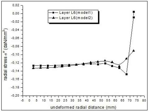
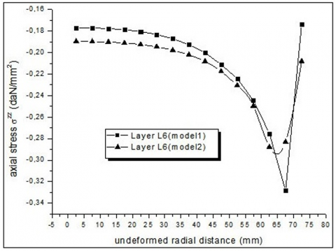
In order to determine the effect of the radial length of the steel plates on the stress field in the elastomer, here the elastomeric layer L6 which has in the (CLEB-model1) this additional elastomeric finite element mentioned above is considered, but which does not have it in the (CLEB-model2).
Figures 16-19 show the evolution of the four physical Cauchy stresses in this elastomeric layer, with a significant increase in the maximum of stresses in absolute value in the model1, and this maximum is always located near the edge of the bearing.
The exploration of the other elastomeric layers revealed similar effects. It will certainly be necessary to consider a more in-depth study in a design office, to determine the most constrained areas in the elastomer, and avoid bearing failure, by application of limit stress criteria and fracture mechanics criteria.
Figure 14. Cylindrical laminated elastomeric bearing (CLEB-model2)
Figure 15. Axisymmetric FE mesh of (CLEB-model2) modeled by 225 four-node finite elements
Figure 16. Effect of the steel plate’s radial length on radial stress in the elastomer
Figure 17. Effect of the steel plate’s radial length on tangential stress in the elastomer
Figure 18. Effect of the steel plate’s radial length on axial stress in the elastomer
Figure 19. Effect of the steel plate’s radial length on shear stress in the elastomer
This paper presented the elements necessary for the implementation of finite element software, for the study of axisymmetric and plane strains in incompressible finite elasticity. The numerical model proposed is based on an intermediate variational formulation, with two fields functional (displacement and hydrostatic pressure), which allows by adopting an adequate approximation for the pressure field, to lead to an incremental system, whose resolution is made only on the field of displacement, by the method of Newton-Raphson. This model differs from the penalty models presented in the literature by the fact that it is deduced from a mixed principle and does not use the reduced integration technique. This avoids the high computational cost generated by mixed methods and the numerical solution divergence problems generated by the reduced integration technique in penalty models.
To prove the good convergence of the model, a study to evaluate the impact of the approximation of the hydrostatic pressure, on the convergence of the numerical solution is carried out. It turned out that the incompressibility parameter ɛ in this approximation (Eq. (7)) must be of the order of 10-4 for optimal convergence. It should be noted here that this problem of convergence of the numerical solution in hyperelasticity, has not been treated before in the literature in the way have approached it in this work.
After the convergence study of the numerical solution, the model was applied to the study of a cylindrical thrust bearing where the exploration of the laminated part of the product made it possible to discover the evolution of the stresses in the elastomer layers where a possible crack may appear. The effect of the dimensional configuration of the steel plates on the mechanical behavior of the bearing was also studied. This study was initiated as part of an approach which aims to isolate the influence of the various parameters acting on the overall behavior of the bearing in operation, knowing that there are other factors to be taken into account in a design study aimed at increasing the performance of the product, in particular the choice of elastomer, and the fixing conditions to the supports.
The future perspectives of this work on the theoretical level would be to extend the model developed here, to three-dimensional strains, and in particular for 3D solids with geometry of revolution subjected to non-symmetrical loadings, using a treatment by Fourier series. Similarly, on a practical level in CAD, it is possible to apply the model in the analysis of the behavior of spherical laminated thrust bearings for the main rotor of a helicopter in aerospace and for the analysis of the behavior of the bearings of bridges in civil engineering.
|
ABAQUS |
Computational software |
|
ANSYS |
Computational software |
|
CAD |
Computer-aided design |
|
CAMMHY |
Computational software |
|
CLEB |
Cylindrical laminated elastomeric bearing |
|
CV error |
Convergence error |
|
CV Iter |
Convergence iteration |
|
EB |
Elastomeric bearings |
|
LRB |
Lead-rubber bearings |
|
NLROM |
Nonlinear reduced-order model |
|
PBR |
Poly-butadiene rubber |
|
SBR |
Styrene-butadiene rubber |
|
XFEM |
Extended finite element method |
|
C1, C2 |
Materials constants (N/mm2) |
|
F |
Applied external load (daN) |
|
pi |
Applied internal pressure (N/mm2) |
|
Re |
Undeformed external radius (mm) |
|
Ri |
Undeformed internal radius (mm) |
|
σrr |
Physical radial stress (N/mm2) |
|
σθθ |
Physical tangential stress (N/mm2) |
|
σzz |
Physical axial stress (N/mm2) |
|
σrz |
Physical shear stress (N/mm2) |
|
List of symbols |
|
|
[Bi] |
Displacements–linear strains transformation matrix |
|
Cijkl |
Elasticity coefficients |
|
[C] |
Elasticity matrix |
|
(CN) |
Deformed configuration |
|
Eij |
Components of the green strain tensor |
|
eij |
Linear part of physical strain |
|
fi |
Elementary volume loads |
|
{F} |
Internal load vector |
|
[G] |
Incompressibility effects matrix |
|
G(I3) |
Function of the invariant I3 |
|
I |
Total element nodes number |
|
I1,I2,I3 |
Cauchy strains tensor invariants |
|
[K(u,p)] |
Stiffness matrix |
|
[KL] |
Large deformation stiffness matrix |
|
[KNL] |
Initial stresses stiffness matrix |
|
[KINC] |
Stiffness matrix of the effects of Incompressibility |
|
[Li] |
Transformation matrix from Vector {δ} to vector {∂u} |
|
p |
Hydrostatic pressure |
|
p0 |
Initial hydrostatic pressure |
|
{R(u)} |
{External nodal load vector |
|
ri |
Deformed internal radius |
|
Sij |
Components of Piola-Kirchoff stress tensor |
|
{S} |
Piola-Kirchoff stresses vector |
|
[S] |
Initial stresses matrix |
|
ti |
Elementary surface loads |
|
u |
Displacement field |
|
ur |
Radial displacements |
|
$\tilde{u}_r$ |
Internal radial displacements |
|
$u_{\alpha_i}$ |
Nodal displacements |
|
V0 |
Undeformed body volume |
|
$V_0^e$ |
Undeformed elementary volume |
|
W |
Strain energy density function |
|
W* |
Modified strain energy density function |
|
Γ0 |
Undeformed body surface |
|
{∆u} |
Nodal displacement increments vector |
|
{δ} |
Elementary vector of nodal displacements |
|
{∂u} |
Vector of first derivatives of displacements |
|
εij |
Physical green deformation (strain tensor) |
|
ε |
Degree of incompressibility factor |
|
ηij |
Nonlinear part of the physical strain tensor |
|
π |
Modified potential energy |
|
ρ0 |
Non-deformed state mass density |
|
σij |
Physical Cauchy stresses (stress tensor) |
[1] Turner, M.J., Dill, E.H., Martin, H.C., Melosh, R.J. (1960). Large deflections of structures subjected to heating and external loads. Journal of the Aerospace Sciences, 27(2): 97-106. https://doi.org/10.2514/8.8412
[2] Becker, E.B. (1966). Numerical solution of a class of problems of finite elastic deformations, Thesis, University of California, Berkeley, California.
[3] Oden, J.T. (1967). Numerical formulation of nonlinear elasticity problems. Journal of the Structural Division, 93(3): 235-255. https://doi.org/10.1061/JSDEAG.0001699
[4] Truesdell, C., Toupin, R. (1969). The Classical Field Theories, Encyclopedia of Physics. Springer, Berlin, Vol. III/I, pp. 600-602.
[5] Herrmann, L.R. (1965). Elasticity equations for incompressible and nearly incompressible materials by a variational theorem. AIAA Journal, 3(10): 1896-1900. https://doi.org/10.2514/3.3277
[6] Scharnhorst, T., Pian, T.H. (1978). Finite element analysis of rubber-like materials by a mixed model. International Journal for Numerical Methods in Engineering, 12(4): 665-676. https://doi.org/10.1002/nme.1620120410
[7] Batra, R.C. (1980). Finite plane strain deformations of rubberlike materials. International Journal for Numerical Methods in Engineering, 15(1): 145-156. https://doi.org/10.1002/nme.1620150112
[8] Oden, J.T. (1978). A theory of penalty methods for finite element approximations of highly nonlinear problems in continuum mechanics. Computers & Structures, 8(3-4): 445-449. https://doi.org/10.1016/0045-7949(78)90189-X
[9] Zdunek, A.B., Bercovier, M. (1986). Numerical evaluation of finite element methods for rubber parts. SAE Transactions, 95(4): 257-269.
[10] Stein, E., Sagar, G. (2008). Convergence behavior of 3D finite elements for Neo-Hookean material. Engineering Computations, 25(3): 220-232. https://doi.org/10.1108/02644400810857065
[11] Baroli, D., Quarteroni, A., Ruiz-Baier, R. (2013). Convergence of a stabilized discontinuous Galerkin method for incompressible nonlinear elasticity. Advances in Computational Mathematics, 39: 425-443. https://doi.org/10.1007/s10444-012-9286-8
[12] Karoui, A., Mansouri, K., Renard, Y., Arfaoui, M. (2014). The extended finite element method for cracked hyperelastic materials: A convergence study. International Journal for Numerical Methods in Engineering, 100(3): 222-242. https://doi.org/10.1002/nme.4736
[13] Mei, Y., Hurtado, D.E., Pant, S., Aggarwal, A. (2018). On improving the numerical convergence of highly nonlinear elasticity problems. Computer Methods in Applied Mechanics and Engineering, 337: 110-127. https://doi.org/10.1016/j.cma.2018.03.033
[14] Farrell, P.E., Gatica, L.F., Lamichhane, B.P., Oyarzúa, R., Ruiz-Baier, R. (2021). Mixed Kirchhoff stress–displacement–pressure formulations for incompressible hyperelasticity. Computer Methods in Applied Mechanics and Engineering, 374: 113562. https://doi.org/10.1016/j.cma.2020.113562
[15] Chavan, K.S., Lamichhane, B.P., Wohlmuth, B.I. (2007). Locking-free finite element methods for linear and nonlinear elasticity in 2D and 3D. Computer Methods in Applied Mechanics and Engineering, 196(41-44): 4075-4086. https://doi.org/10.1016/j.cma.2007.03.022
[16] Barnafi, N.A., Pavarino, L.F., Scacchi, S. (2022). Parallel inexact Newton–Krylov and quasi-Newton solvers for nonlinear elasticity. Computer Methods in Applied Mechanics and Engineering, 400: 115557. https://doi.org/10.1016/j.cma.2022.115557
[17] Hong, Q., Liu, C., Xu, J. (2020). An abstract stabilization method with applications to nonlinear incompressible elasticity. arXiv Preprint arXiv:2005.00189. https://doi.org/10.48550/arXiv.2005.00189
[18] Kadapa, C., Hossain, M. (2022). A linearized consistent mixed displacement-pressure formulation for hyperelasticity. Mechanics of Advanced Materials and Structures, 29(2): 267-284. https://doi.org/10.1080/15376494.2020.1762952
[19] Fradet, A. (2023). Fracture simulation with a hyperelastic phase field model. Thesis, KTH Royal Institute of Technology, Stockholm, Suede.
[20] Prabhune, B., Suresh, K. (2023). Isoparametric tangled finite element method for nonlinear elasticity. arXiv Preprint arXiv:2303.10799. https://doi.org/10.48550/arXiv.2303.10799
[21] Mountris, K.A., Li, M., Schilling, R., Dong, L., Atluri, S.N., Casals, A., Wurdemann, H.A. (2023). An explicit total Lagrangian fragile points method for finite deformation of hyperelastic materials. Engineering Analysis with Boundary Elements, 151: 255-264. https://doi.org/10.1016/j.enganabound.2023.03.001
[22] Luo, H., Zhu, Y., Zhao, H., Ma, L., Zhang, J. (2023). Equibiaxial planar tension test method and the simulation analysis for hyperelastic EAP membrane. Advances in Polymer Technology, 2023(1): 7343992. https://doi.org/10.1155/2023/7343992
[23] Canales, C., García-Herrera, C., Rivera, E., Macías, D., Celentano, D. (2023). Anisotropic hyperelastic material characterization: Stability criterion and inverse calibration with evolutionary strategies. Mathematics, 11(4): 922. https://doi.org/10.3390/math11040922
[24] Kalfas, K.N., Mitoulis, S.A., Konstantinidis, D. (2020). Influence of steel reinforcement on the performance of elastomeric bearings. Journal of Structural Engineering, 146(10): 04020195. https://doi.org/10.1061/(ASCE)ST.1943-541X.0002710
[25] Mazza, F., Mazza, M. (2020). Influence of elastomeric bearings in tension on the seismic performance of base-isolated RC buildings. Applied Sciences, 11(1): 82. https://doi.org/10.3390/app11010082
[26] Han, D., Che, W. (2021). Comparison of the shear modulus of an offshore elastomeric bearing between numerical simulation and experiment. Applied Sciences, 11(10): 4384. https://doi.org/10.3390/app11104384
[27] Leblouba, M. (2022). Stability analysis of elastomeric bearings in bridge structures. Advances in Bridge Engineering, 3(1): 11. https://doi.org/10.1186/s43251-022-00062-1
[28] Premnath, M., Gopi, K.K. (2023). Experimental and numerical analysis of the performance of various damper materials. Trends in Sciences, 20(8): 5038-5038. https://doi.org/10.48048/tis.2023.5038
[29] Gadala, M.S., Dokainish, M.A., Oravas, G.A. (1980). Geometric and material nonlinearity problems: Lagrangian and updated Lagrangian formulations. International Journal of Non-Linear Mechanics, 277-293.
[30] Häggblad, B., Sundberg, J.A. (1983). Large strain solutions of rubber components. Computers & Structures, 17(5-6): 835-843. https://doi.org/10.1016/0045-7949(83)90097-4
[31] Green, A.E., Zerna, W. (1968). Theoretical Elasticity. Oxford University Press, London, p. 458.
[32] Masrar, M. (2005). Conception et Analyse des Matériaux Hyperélastiques (CAMMHY), Guide de l’utilisateur, USMBA, FSTF, Morocco, Internal Report. https://fst-usmba.ac.ma/laboratoire_msm/.
[33] Masrar, Y., Ettaouil, M. (2021). A nonlinear plane strain finite element analysis for multilayer elastomeric bearings. Applied Mathematics and Computation, 404: 126218. https://doi.org/10.1016/j.amc.2021.126218
[34] Fediuc, D.O., Budescu, M., Baetuand, S., Fediuc, V. (2015). Finite element modeling of elastomeric bearings. Buletinul Institutului Politehnic Din Iaşi, Universitatea Tehnică, Gheorghe Asachi, din IaşiTomul LXI (LXV), Fasc. 2. https://www.bipcons.ce.tuiasi.ro/Archive/508.pdf.
[35] Guzman, M.A., Forcellini, D., Moreno, R., Giraldo, D.H. (2018). Theoretical, numerical and experimental assessment of elastomeric bearing stability. International Journal of Architectural and Environmental Engineering, 12(11): 1083-1088.
[36] Forcellini, D. (2016). 3D numerical simulations of elastomeric bearings for bridges. Innovative Infrastructure Solutions, 1: 1-9. https://doi.org/10.1007/s41062-016-0045-4