Halkawt R. Hussein![]() | Sarkawt R. Hussein
| Sarkawt R. Hussein![]() | Adel S. Hussain
| Adel S. Hussain![]() | Mohammad A. Tashtoush*
| Mohammad A. Tashtoush*![]()
© 2025 The authors. This article is published by IIETA and is licensed under the CC BY 4.0 license (http://creativecommons.org/licenses/by/4.0/).
OPEN ACCESS
In this paper, the software reliability growth model of Rayleigh Order Statistics distribution, formulated under the Non-Homogeneous Poisson Process (NHPP) model, is presented. This model seeks to include new approaches in the data analysis to improve the reliability of the software reliability predictions taking into consideration the various issues of failure data. For parameter estimation, a hybrid Artificial Neural Network (ANN) model is introduced, which has been trained by the Artificial Bee Colony (ABC) algorithm, and the analysis shows that such a model yields much better results in predictive performance. The research assesses the performance of the developed model based on actual software reliability data sets and demonstrates the superiority of the proposed model to conventional NHPP models in goodness-of-fit and predictive accuracy. Further, the study reveals some of the deficiencies with the current models and the significance of accurate failure data in the analysis of reliability; also, the paper recommends the recognition and incorporation of higher levels of intelligent calculations in future work. These findings add practical value to further developments in software engineering, especially in increasing the effectiveness of quality assurance and extending the durability of software applications.
Rayleigh Order Statistics process, software reliability growth model, Non-Homogeneous Poisson Process, unconstrained optimization technique, Artificial Neural Network, Artificial Bee Colony, simulation
In the fast-paced realm of modern technology, ensuring the reliability of software systems is crucial for maintaining operational efficiency and achieving user satisfaction [1, 2]. Software failures can result in substantial financial repercussions, security vulnerabilities, and a loss of user trust. Consequently, the development of robust Software Reliability Growth Models (SRGMs) is vital for accurately predicting and enhancing software performance throughout its lifecycle [3-6].
In today’s software world, software dependability is a critical objective in software construction. Multi Var Time Series Software Reliability Growth Models Losses occur if software fails to meet the customers’ expectations, poses insecurities, and loses users’ confidence hence the need for developers to incorporate effective SRGMs. As will be discussed, these models are invaluable in the context of software performance prediction and improvement across the software development life-cycle. With an even more complex structure of applications being developed every passing day, there has been growing pressure for even better modeling methods that can capture software failure behavior [7-10].
The Non-Homogeneous Poisson Process, abbreviated as (NHPP) has increasingly become a popular choice for software reliability modeling [11]. This approach enables one to express the failure occurrences with time and enables one to capture changes in failing rates resulting from differences in operating conditions. The new developments in future work have incorporated Order Statistics distributions, namely Rayleigh distribution, in presenting better reliability features to software systems. These distributions help the researchers to understand failure data better and consequently make accurate predictions of the software’s performance [12-14].
Besides statistical methods, the use of new methods like Machine Learning methods, particularly Artificial Neural Networks (ANN) has also been incorporated in software reliability modeling [15, 16]. The integration of ANN with optimization algorithms like the Artificial Bee Colony (ABC) algorithm has proved to improve parameter estimation techniques incorporated in SRGMs. This innovative approach not only enhances the accuracy of the predictors but is also capable of dealing with massive and complicated data and information that are universal in software applications [17-19].
Nevertheless, there are some issues with the application of software reliability modeling even if certain improvements can be seen. While using such models, the assumptions made are often not well adaptable to diverse software systems in their current form. Precisely, the quality and representativeness of failure data play important roles in determining the performance of these models. Finally, situations, when the data is scarce or contaminated, affect the reliability predictions, which proves the importance of developing stronger techniques suitable for software systems.
This research seeks to fill gaps found in existing models of software reliability including the failure to capture intricate patterns that vary with time. Through this work, a new model within the NHPP framework, incorporating the Rayleigh Order Statistics of software reliability, and ANN-ABC principles for parameter estimation has been developed. These more advanced methods improve the capability of the software reliability models and make them more general for many software systems. The results of the study should encourage further development of software engineering research in the aspect of improving quality assurance as well as the prolongation of software systems’ life cycle.
1.1 Literature review
In 2017, the researchers proposed a new NHPP software reliability model with an S-shaped growth curve that accounts for random operating environments. They aimed to improve predictions of software defects, optimize release times, and minimize overall software system costs during the development process [20].
Furthermore, in 2019, the researchers developed a new software reliability growth model based on the Weibull Order Statistics distribution and the NHPP. They created an algorithm and a MATLAB program for practical implementation, employed maximum likelihood estimation for parameter estimation, and analyzed software failure data to validate the model. Additionally, they suggested future research directions involving advanced optimization techniques to enhance reliability predictions [21].
In 2022, the researchers proposed a hybrid meta-heuristic approach combining Ant Colony Optimization (ACO) with the BAT Algorithm (HACO-BA) to optimize deep learning models for software cost estimation. Their work focused on improving the accuracy of software cost predictions by fine-tuning COCOMO II coefficients and enhancing deep learning model training. By comparing various optimization algorithms, including ACO, BAT, and HACO-BA, the researchers demonstrated that HACO-BA provided better performance in terms of minimizing execution time and improving prediction accuracy [22].
In 2023, all the researchers in this article aimed to apply the NHPP reliability growth model to assess failure data in repairable systems. They explored and estimated various models such as the Crow Power Law model and also conducted tests for goodness of fit. This also involved using a log-linear model when results from the Power Law model were and/or could not adequately fit. Moreover, the utilization of the Weibull Time to Failure Recurrent Neural Network (WTTE-RNN) framework was attempted but not viable for some types of NHPP data [23].
In 2024, the researchers propose a finite failure software reliability model based on the extended log-logistic distribution within the framework of the NHPP. They derived the model's properties, applied the maximum likelihood estimation method to estimate its parameters using the Newton-Raphson method, and evaluated the model with three real software reliability datasets. The results show that the proposed model outperformed several well-known NHPP models in terms of goodness-of-fit and predictive performance across all datasets [24].
Future trends for SRGM are aimed mainly at the improvement of the accuracy of prediction, flexibility of models, and applicability of the modeling approaches in practice. These include the application of artificial intelligence and machine learning for enhanced prediction as well as the use of real-time failure data to enhance model responsiveness. It has been observed that modern mixed models that integrate statistical and machine learning methods have been evolving. Further, the focus has shifted to the collection of user-oriented reliability measures, like user satisfaction level and user experience. Finally, efforts are made to get more empirical evidence to prove models on different software systems and environments which remains a challenge for developing more advanced SRGMs to fulfill the demands of modern software engineering.
1.2 Limitations of the NHPP model for Rayleigh Order Statistics in SRGM
Model assumptions: The proposed reliability growth model is based on specific assumptions inherent to the Rayleigh process and the NHPP. These assumptions may not hold for all software systems or failure scenarios, potentially limiting the model's applicability in diverse contexts.
Data dependency: The effectiveness of the Weibull order statistics distribution in modeling software reliability is contingent upon the quality and quantity of failure data available. In cases where data is sparse or not representative of the software's operational environment, the model's predictions may be less reliable.
Complexity of real-world systems: Real-world software systems often exhibit complex behaviors that may not be fully captured by the proposed model. Factors such as user interactions, environmental conditions, and varying usage patterns can influence software reliability in ways that are difficult to quantify.
Computational resources: The implementation of the algorithm and MATLAB program may require significant computational resources, especially when dealing with large datasets or complex models. This could pose challenges for practitioners with limited access to advanced computational tools.
Limited scope of optimization techniques: Although the paper suggests the integration of advanced optimization techniques like ANN and ABC for future research, the current study does not explore these methods in depth. The potential benefits of these techniques remain theoretical until empirically validated in the context of software reliability.
Generalizability: The findings and methodologies presented may be specific to the datasets used in the study. Generalizing the results to other software systems or industries may require further validation and testing.
Focus on quantitative metrics: The model primarily emphasizes quantitative reliability metrics, potentially overlooking qualitative aspects of software reliability, such as user experience and satisfaction, which are also critical for assessing overall software performance.
By tackling the pressing need for dependable software systems, this research contributes significantly to the ongoing advancements in software engineering, particularly in enhancing quality assurance practices and prolonging the operational lifespan of software applications. The insights and methodologies presented in this work are intended to serve as a valuable resource for both researchers and practitioners, promoting further progress in the domain of software reliability.
This paper introduces an innovative approach to assessing software reliability by formulating a growth model based on the Rayleigh Order Statistics distribution, anchored in the NHPP. The Rayleigh process is esteemed for its adaptability in modeling diverse failure rates, making it particularly suitable for addressing the intricacies of software reliability. By utilizing order statistics, this model establishes a comprehensive framework for analyzing failure data and estimating key reliability metrics.
Moreover, the paper advocates for the incorporation of advanced optimization techniques, such as the combination of ANN and ABC, in future research endeavors. This synergistic approach holds promise for enhancing parameter estimation processes, thereby yielding more precise predictions of software reliability.
1.3 Theoretical foundations of Software Reliability Growth Model
Software reliability growth modeling is an important sub-discipline of software engineering that deals with the prediction and enhancement of the reliability of software systems in the software development life-cycle stages. SRGMs apply statistical assessments to the failure data collected, allowing the developer to predict the remaining defective items and the reliability level of the software in use. SRGMs can also serve as a guide to defining the improvement of reliability when defects are found and fixed to facilitate better planning of release times, improvement of QA measures, and, consequently, the minimization of expenses connected with software failures. With the developing complexity of the software systems, operational effectiveness and user satisfaction calls for efficient SRGMs.
The main models in Software Reliability Growth Modeling (SRGM) include:
NHPP: This model takes into consideration different failure rates at different times to accommodate for dynamism in environments such as software.
Weibull distribution models: These models effectively provide options for the portrayal of various failure behaviors by holding the capability to portray rising and declining failure rates.
Logarithmic and exponential models: These have been widely adopted since they are easy to apply but often, they lack the capability of modeling complex failure functions.
Hybrid models: These models integrate standard and advanced statistical methods with MLE’s and contribute to improved prognosis and adaptability for increased variable difficulty and data licenses.
Meta-heuristic approaches: Two classes of metaheuristic methods, including Genetic Algorithms and Particle Swarm Optimization, are applied to enhance parameter estimation of SRGMs.
All of these models have some advantages and disadvantages, the decision on which model to use when depends on the nature of the software being analyzed.
The NHPP, which is assumed by the majority of SRGMs, is described by the following equation:
$p[N(t)=y]=\frac{[m(t)]^y e^{-m(t)}}{y!}, y=1,2,3, \ldots$ (1)
It describes the total number of failures up to a specific execution time $t$, shown as $N(t)(t>0)$. The predicted cumulative number of failures at time $t$ is represented by the mean value function $m(t)$, as follows:
$m(t)=\int_0^t \lambda(u) d u, 0<\tau<\infty$ (2)
with $m(t)$ the NHPP-based dependability function may be stated as follows [24]. The likelihood of no failures in the time interval $(0, t)$ is defined as the reliability function $R(t)$, which is provided by:
$R(t)=p\{N(t)=0\}=e^{-m(t)}$ (3)
Reliability $R\left(\frac{y}{t}\right)$ generally indicates the likelihood that there won't be any failures during the period. $[t, t+y]$ is given by:
$R\left(\frac{y}{t}\right)=p\{N(t+y)-N(t)=0\}=e^{-[m(t+y)-m(t)]}$ (4)
Eq. (4) is called the SRGM or software reliability based on NHPP. The probability density functions as follows:
$f(y)=\lambda(\mathrm{t}+\mathrm{y}) e^{-[m(t+y)-m(t)]}$ (5)
Artificial Neural Network is a collection of neurons linked by pathways in which those neurons carry weights and biases. They further explain that once the network structure has been developed, the next process is to exercise the network. The process of setting the weights and biases of the networks to their optimal values is called network training. Typically, one or several techniques are employed in evaluating proper weights and bias for the ANN. In order to get the best result in the training of network, the ABC has been applied in this study. Further information about ABC is available in studies [25, 26], which contains a detailed overview of the ABC approach used in this investigation [27]. Furthermore, there exist the MATLAB implementation codes of the following.
2.1 Proposed Artificial Neural Networks training approach using Artificial Bee Colony algorithm
ANNs are one of the most widely used artificial intelligence tools in applications including classification, prediction, and pattern recognition. Neural networks can perform millions of operations without missing a beat given the right weights and parameters for training. In the past, it was customary to train a neural network using an optimization algorithm for example the gradient descent; this tends to get stuck in a local minimum depending on the loss function space. To overcome these challenges, suggest the ABC algorithm as another innovative approach to training Artificial Neural Networks. The Artificial Bee Colony algorithm is similar to the Fireflies optimization algorithm, where fireflies are attracted by the other based on the light intensity. Six essential phases will be involved in training the ANN with algorithm ABC as follows [28]:
Step 1. Data formatting: collecting and dividing data.
Step 2. Neural network design: determining the structure, activation functions, and loss functions.
Step 3. Initializing the ABC algorithm: Defining the set of fireflies and the brightness function.
Step 4. Training a neural network with ABC: Calculating brightness, updating ABC locations, evaluating performance, and iterating.
Step 5. Validation and final evaluation: Use validation and test suites to evaluate Eq. (18).
Step 6. Implementation and application: Using the trained Eq. (18) in practical applications.
3.1 Mathematical formulations
Software reliability is best described as the ability of a software system to perform without encountering any error over a given duration of operation given certain conditions. Reliability analysis must also be done and quality maintenance of software is highly important in order that the system have the right performance and dependability that is needed. Software Reliability Growth Models therefore stand as key drivers for assessing performance and achieving rigorous debugging in order to improve the durability of the system [29].
A previous model has been developed based on the Rayleigh Order Statistics distribution fit within the NHPP model. This integration enables the model to capture failure rates to increase monotonically with time as observed in realistic software systems. The foundation of the model is the mean value function $m_1(t)$ which is mathematically:
$m_1(t)=\int_0^t \lambda(u) d u$ (6)
where, $\lambda(t)$ denotes the failure intensity function. For a random variable $X$ following a Rayleigh process, the occurrence rate is determined by:
$\lambda(t)=\frac{1}{b^2} t, t \geq 0, b>0$ (7)
where, $b$ represents scale parameter. If we substitute Eq. (7) into Eq. (6) and simplify, then we obtain:
$m_1(t)=\frac{1}{2 b^2} t^2$ (8)
For the stochastic process, the inter-arrival times are determined by Hussain et al. [29]:
$f(t)=\lambda(t) e^{-m\left(t_0\right)}$ (9)
For the Rayleigh process, we may express the probability density function as follows:
$f(t)=\frac{1}{b^2} t e^{-\frac{1}{2 b^2} t_0^2}, t>0$ (10)
The cumulative distribution function for New Process is:
$F(t)=1-e^{-\frac{1}{2 \mathrm{~b}^2} \mathrm{t}_0^2}$ (11)
Suppose that $\left(X_1, \ldots, X_n\right)$, there are n random variables with joint distribution. The $X_{i / s}$ is arranged in ascending order, which represents the order of the corresponding statistics. Thus $X_{1: n} \leq X_{2: n} \leq \cdots \leq X_{n: n}$. An independent, identically distributed sample from a continuous distribution of absolute density $f(x)$ has the joint density function of the order statistics as [30]:
$\begin{gathered}f_{X_{1: n}, \ldots, X_{n: n}}\left(x_1, x_2, \ldots, x_n\right)=n!\prod_{i=1}^n f\left(x_i\right), \\ \infty<x_1<x_2<\cdots<x_n<\infty\end{gathered}$ (12)
NHPP models or fault counting models can be classified into finite or infinite failure models, depending on the specification. In this model, the number of failures follows the distribution of a Non-Homogeneous Poisson Process, and the failure severity function is determined according to this distribution $\lambda_1(x)$ is defined as $\lambda_1(x)=a f(x)$ where $a$ is the number of failures expected and $f(x)$ is the probability density function of $X$. Based on NHPP assumptions, mean value function is $m(x)=a F(x)$, where $F(x)$ is the cumulative distribution function of $X$ and $a=\frac{m(x)}{F(x)}$ [31].
3.2 Properties of the model
The proposed model exhibits the following properties:
Time-dependent failure analysis: The model integrates failure rates that tend to rise over time, factors considered when analyzing software stress and operational usage with the help of the NHPP framework.
Order statistics integration: Order statistics are incorporated into the model in order to model the prospective time until the k-th failure, a parameter, which is essential if the system needs to be repaired more than once.
Adaptability: The model is flexibly designed for accommodating different current operational conditions and different failure patterns making it to suit many scenarios of software reliability.
3.3 Assumptions
The proposed model is based on the following assumptions:
•The software failure process follows Rayleigh distribution of the NHPP model.
•The failure rates rise with time and this is consistent with the behavior experienced with software reliability data.
•Failure data needs to be of high quality and preferably representative of the actual system for accurate identification of the parameters and subsequent prediction of the system.
3.4 New process order statistics growth model
Let $X_1, X_2, \ldots, X_n$ random variables represent a sample of the cumulative time intervals between failures. And let $X_{1: n}, \ldots, X_{n: n}$ the original random variables so that $X_{1: n} \leq$ $X_{2: n} \leq \cdots \leq X_{n: n}$ are called the order statistics. The probability density function of Rayleigh process $r^{\text {th }}$ order statistics is given by:
$\begin{aligned}f_{r: n}(x)= & r\binom{n}{r} \frac{x}{b^2}\left[1-e^{\frac{-x_0}{2 b^2}}\right]^{r-1} e^{-(n-r+1) \frac{x_0 2}{2 b^2}} \\& x \in[0, \infty) ; b>0 ; 1 \leq r \leq n\end{aligned}$ (13)
The $c d f$ is:
$F_{r: n}(x)=\sum_{i=r}^n\binom{n}{i}\left[1-e^{\frac{-x_0{ }^2}{2 b^2}}\right]^r e^{-(n-i) \frac{x_0^2}{2 b^2}}$ (14)
This section describes two techniques for estimating the parameters of the new process order statistics growth model.
4.1 Modified maximum likelihood estimation (MMLE)
Let's look at some software failure data that is expressed as $\left(x_i, t_i\right)$, where $i$ is a number between 1 and $n$. Here, $x_i$ denotes the number of failures that have been seen within the time interval $\left[0, t_i\right]$, where time point's fall into the range $0<t_1<$ $t_2<\ldots<t_n$, usually this kind of information is called "failure count data." The NHPP parameters may be estimated by building a log-likelihood function, which has the following form [32, 33]:
$l=\prod_{i=1}^n r\binom{n}{r} \frac{x_i}{b^2}\left[1-e^{\frac{-x_0 0^2}{2 b^2}}\right]^{r-1} e^{-(n-r+1) \frac{x_0 2}{2 b^2}}$ (15)
The maximum likelihood estimator for the value $b$ can be obtained from Eq. (15), where:
$\begin{gathered}\log l=n \log r+\log \binom{n}{r}+n(r-1) \log \left(1-e^{\frac{-x_0{ }^2}{2 b^2}}\right) \\
-(n-r+1) \frac{x_0^2}{2 b^2}+\sum_{i=1}^n \log \left(\frac{x_i}{b^2}\right)\end{gathered}$ (16)
This equation can be solved numerically using iterative methods such as the Newton-Raphson algorithm or the EM algorithm to obtain estimates of the parameter $b$ that maximize the likelihood function [34, 35]. We find that solving the equation derived from Eq. (16) with respect to $b$ is not possible using conventional methods due to the high degree of nonlinearity. Therefore, we propose a modified method to achieve the maximum likelihood by combining the ANN technique with the ABC algorithm.
4.2 NHPP Model for Rayleigh Order Statistics SRGM
The mean value function for this SRGM, using Eq. (9) is:
$m(x)=a \sum_{i=r}^n\binom{n}{i}\left[1-e^{\frac{-x_0^2}{2 b^2}}\right]^r e^{-(n-i) \frac{x_0^2}{2 b^2}}$ (17)
The intensity value function, using Eq. (8) is:
$\lambda_1(x)=\operatorname{ar}\binom{n}{r} \frac{x}{b^2}\left[1-e^{\frac{-x_0{ }^2}{2 b^2}}\right]^{r-1} e^{-(n-r+1) \frac{x_0 2}{2 b^2}}$ (18)
where, $a$ the expected number of failures. Then
$a=\frac{n}{\sum_{i=r}^n\binom{n}{i}\left[1-e^{\frac{-x_0^2}{2 b^2}}\right]^r e^{-(n-i) \frac{x_0^2}{2 b^2}}}$ (19)
Figure 1. Flowchart of ANN-based ABC
4.3 ANN-ABC algorithm for parameter estimation in new process order statistics SRGM
This algorithm identifies the process of preparing the input data for the neural network as well as the way of initialization and training of ANN model. All the input variables are factors that describe the data Set, which in most cases refers to the independent variables. All these inputs are forwarded into the neurons in the input layer of the devised neural network. Before we begin the training process, we have to set the weights and biases of the neural network. This is normally done at random and can be from a uniform distribution as well select (random), here this needs to be done randomly normally distribution Weights denote the connection of neurons in different layers and bias brings for each neuron a new internal parameter for regulating the output [36].
After the weights and the bias are initialized, the data is passed forward through to the network. In this case, the weights are in the range of 0.001 to 0.009 while the bias is always greater than 0. In the hidden layer, each neuron processes input from the input layer in the manner mentioned above where the weighted sum is calculated using the weight factor and additional bias factor accompanied by the activation function to generate an output. After that, we chose a multilayer FFNN that contains two hidden layers: one input and one output. The first hidden layer is comprised of six nods and the second one is comprised of nine nods. These experiments showed us that the network topology with two hidden layers produces better results than with one and three hidden layers. In particular, when using 6 nodes in the first hidden layer and 9 nodes in the second hidden layer, this configuration showed statistically significant superiority; the output of the neural network is then tested against the actual target values using a loss function.
For example, in this case, the most widely used measure is the root mean squared error (RMSE). Thus, it can be concluded that lower MSE means that the shown model and structure of the neural network correspond to the described task of approximating the target values as much as possible. This process has to be carried out until the model returns a satisfactory performance or until a predefined stop has been reached. Theis’s process is summarized by the following steps [37]:
Step 1. Initialize ANN
Step 2. Initialize ABC
Step 3. Evaluate ANN
Step 4. Employed bees phase
Each employed bee searches for a new food source (solution) in the neighborhood of its current position using the following equation:
$v_{i j}=x_{i j}+\pi_{i j} *\left(x_{i j}-x_{k j}\right)$ (20)
where,
$v_{i j}$ is the new food source (solution).
$x_{i j}$ is the current position of the employed bee.
$\pi_{i j}$ is a random number between -1 and 1.
$x_{k j}$ is the position of a randomly selected bee $k$.
Step 5. Onlooker bees phase
Each onlooker bee selects a food source (solution) from the employed bees based on the probability.
Step 6. Scout bees phase
If a food source (solution) is abandoned, a scout bee is sent to search for a new food source using the following equation:
$x_{i j}=x_{\min , j}+\operatorname{rand}(0,1) *\left(x_{\max , j}-x_{\min , j}\right)$ (21)
where,
$x_{i j}$ is the new food source (solution).
$x_{\max , j}$ and $x_{\min , j}$ are the minimum and maximum bounds of the $j^{\text {th}}$.
Step 7. Once the weights and biases have been updated, check the mean square error. If $M S E_{\text {new }} \leq M S E_{\text {old }}$, then choose $M_{\text {new }}=M_{\text {old }} / B$ and go to step 2. Otherwise choose $M_{\text {new }}=M_{\text {old }} * B$ and go to step 3.
Step 8. Iteration
Repeat steps 3-7 until a stopping criterion is reached. Then a flowchart of ANN training with the ABC algorithm is given in Figure 1 [38].
Simulation is a scenario designed to compare any system with the real world, and is defined as the attempt to simulate a particular process under specific circumstances using artificial methods that resemble natural conditions. This includes building a smaller model that is an identical copy of the real model and performing tests on the miniature model examining the results and generalizing them to the original model, or computer simulation by writing a program for the methods to be chosen under realistic programming conditions and then observing the results obtained with the program and drawing a conclusion based on them [37, 39].
There are different simulation methods, namely the (analog method), the (mixed method) and the (Monte Carlo method). The Monte Carlo method is one of the most important and widely used simulation methods, in which a random sample of the phenomenon is generated, that corresponds to the behavior of a certain probability distribution that the phenomenon has. To achieve this, the probability distribution of the phenomenon it has (CDF) it is known that the set of samples random in this way possesses the property of independence because random samples in this method are by applying the mathematical method to each sample separately [38-40].
To put the previously discussed ideas into practice, the practical part of the research focused on the estimators of the suggested model for both of the approaches used, utilizing a simulation method. The objective was to apply the RMSE statistical criteria to various sample sizes in order to assess the optimality of these estimators. The purpose of the simulation model was to provide a comparison study of the approaches that were evaluated. By showing how the estimate techniques affect the following variables, this strategy seeks to determine the best technique for estimating parameters inside the interval of the new process distribution [39].
5.1 Stages of building a simulation experience
First stage: Parameter value selection: Many of the default values were selected based on prior studies and experimental tests ($a=1.9 ; 0.9 ; 1.2 ; 1.1$ and $b=0.9 ; 1.2 ; 1.1 ; 1.9$), with statistical methods such as modified maximum likelihood estimation and an enhanced neural network optimized using the ABC algorithm employed to determine the optimal parameter values. It is the most important stage on which the program’s steps and procedures depend. Below are the steps for this stage:
Choose default values for the parameters of the new process. Several default values were chosen for the failures expected parameter a and the scale parameter b for the new process by reviewing previous studies and experimenting with many default values for the parameters, which led us to choose the best of these values, as follows above.
Second stage: Choose sample sizes: Several different sample sizes (small, medium, large) were chosen as follows: ($n=20 ; 50$).
Third stage: Number of replications: The simulation was repeated 1000 times to obtain reliable estimates and to account for the variability in the data to achieve a balance between computational efficiency and statistical reliability.
Fourth stage: Performance metrics: Root Mean Square Error (RMSE) measure was used. To evaluate the accuracy of parameter estimates. It is calculated as
$R M S E=\sqrt{\frac{\sum_{i=1}^Q\left(\widehat{\gamma}_l-\gamma\right)^2}{Q}}$
where,
$\widehat{\gamma}_l$: represents value of the parameter estimated in iteration $i$.
$\gamma$: represents the real parameter value.
$Q$: represents number of iterations.
In the context of the study, RMSE quantifies the difference between the observed software failure data and the values predicted by the proposed model. The smaller the RMSE, the closer the predictions are to the actual data, indicating better model performance.
Fifth stage: Data generation: At this stage, random data is generated using the inverse transformation method and according to the new process, as follows:
Generating a random variable $u_i$ that follows a uniform distribution with the interval $(0,1)$ using the cumulative distribution function with the help of the Rand.
$u_i \sim U(0,1), i=0,1,2, \ldots \ldots, n$ (22)
where, $u_i$ represents a continuous random variable that follows a uniform distribution.
Convert the data generated in step (first) that follows a uniform distribution into data that follows a new mixed distribution using the inverse function (CDF) transformation method and according to Eq. (17) and as in the following formula.
$t_i=\sqrt{2 b^2 * \ln \left(1-\frac{u}{a}\right)}, i=0,1,2, \ldots, n$ (23)
Sixth stage: At this stage, parameters are estimated over the period for the new process and for all methods, which are MMLE, and ANN-ABC.
Seventh stage: The experiment is repeated (1000) times.
5.2 Simulation result
After conducting the simulation experiment by implementing the program in the electronic calculator, the results of the parameter estimate for the new mixed Rayleigh distribution were obtained using the two estimation methods described in the above sections and the RMSE. The results of the simulation estimations were presented in Table 1 in order to reach the best estimate. Comparison between the studied estimation methods. In simulating the proposed model, parameters a and b were chosen based on empirical evidence from prior studies and sensitivity analysis to balance model accuracy and computational efficiency. The values different a, and b were selected for their effectiveness in minimizing RMSE and capturing observed failure characteristics.
Table 1. Simulated RMSE comparison of MMLE and ANN-ABC estimates for new process parameters
|
$n$ |
Parameters |
Methods |
$R M S E\left(\widehat{\lambda_1}(x)\right)$ |
|
20 |
$\{a=0.5 ; b=0.6\}$ |
MMLE |
0.0843 |
|
ANN-ABC |
0.0765 |
||
|
$\{a=0.6 ; b=0.5\}$ |
MMLE |
0.0664 |
|
|
ANN-ABC |
0.0096 |
||
|
$\{a=0.6 ; b=0.7\}$ |
MMLE |
0.1339 |
|
|
ANN-ABC |
0.0549 |
||
|
50 |
$\{a=0.5 ; b=0.6\}$ |
MMLE |
0.0836 |
|
ANN-ABC |
0.0738 |
||
|
$\{a=0.6 ; b=0.5\}$ |
MMLE |
0.0848 |
|
|
ANN-ABC |
0.0778 |
||
|
$\{a=0.6 ; b=0.7\}$ |
MMLE |
0.0847 |
|
|
ANN-ABC |
0.0779 |
The real-world dataset we use is derived from reference [21] and represents failure attributes including failure time stamp, failure type, and operational conditions, which truly demonstrate various failure characteristics and are suitable for model testing. When the produced model is checked against this dataset,
The real-world dataset we use is derived from reference [21] and represents failure attributes including failure time stamp, failure type, and operational conditions, which truly demonstrate various failure characteristics and are suitable for model testing. When the produced model is checked against this dataset, one can determine how well it performs on real-world software reliability and failure patterns hence making it quite practical on software quality enhancement.
Forming a dataset originating from the software system, Table 2 shows a time split-up of failure intervals and their cumulative time [22]. This information is essential for detecting and assessing system efficiency and reliability issues while offering statistics describing previous failures. In particular, it is possible to observe that some measured failure intervals are rather long – 125.67 CPU units between the 17 and 18th failures – while others are short, meaning that the tested software can be characterized by different levels of reliability in the course of its functions. These datasets can be used to prove the adequacy of the SRGM models based on the proposed NHPP model through graphical analysis.
Besides providing insights into the software’s operational characteristics, this dataset has been used to proffer recommendations that may be useful in tuning the software further in the future. These include the following: The best of these insights is to improve software dependability, lessen the frequency of outages, and advance development and maintenance practices [22].
Secondly, the datasets are graphically examined to investigate their suitability for the new process in SRGM. This is achieved by plotting the distribution using an Artificial Neural Network, as shown in Figure 2.
The histogram of cumulative failures at day of the specific dataset under analysis is represented in the form of the graphical logarithmic function in Figure 2. The scatter diagram shows an obvious positive linearity; this is good evidence for utilizing a mean value function to model this data. To strengthen this modeling, a novel data analysis model based on an Artificial Neural Network optimized through an Artificial Bee Colony algorithm (ANN-ABC) has been used to improve the predictive accuracy of the proposed model [41-44].
Table 2. The cumulative time between failures
|
Failure Number |
Time Between Failure Times in CPU Units |
Cumulative Time Between Failures |
|
1 |
5.5 |
5.5 |
|
2 |
1.83 |
7.33 |
|
3 |
2.75 |
10.08 |
|
4 |
70.89 |
80.97 |
|
5 |
3.94 |
84.91 |
|
6 |
14.98 |
99.89 |
|
7 |
3.47 |
103.36 |
|
8 |
9.96 |
113.32 |
|
9 |
11.39 |
124.71 |
|
10 |
19.88 |
144.59 |
|
11 |
7.81 |
152.4 |
|
12 |
14.59 |
166.99 |
|
13 |
11.42 |
178.41 |
|
14 |
18.94 |
197.35 |
|
15 |
65.3 |
262.65 |
|
16 |
0.04 |
262.69 |
|
17 |
125.67 |
388.36 |
|
18 |
82.69 |
471.05 |
|
19 |
0.45 |
471.5 |
|
20 |
31.61 |
503.11 |
|
21 |
129.31 |
632.42 |
|
22 |
47.6 |
680.02 |
Table 3. Models t-test
|
Models |
t |
d.f. |
Mean Difference |
Std. Error Difference |
|
Weibull model |
3.284 |
108 |
0.533 |
0.166 |
|
Suggested model |
3.217 |
107.817 |
0.533 |
0.162 |
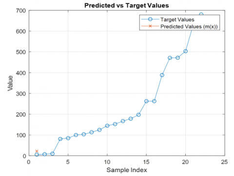
Figure 2. Target vs. predicted output
The t-test of comparing the proposed model with the Weibull model is presented in Table 3, where t-value is compared with degrees of freedom, mean difference, and standard errors. The t-value of the proposed model is 3.217 with 107.817 degree of freedoms and there is t-value 3.284 with 108 degrees of freedoms of Weibull model. The models indicate a mean difference of 0.533 with the proposed model having slightly higher standard error of 0.162 and the Weibull model having a standard error of 0.166. These results verify the proposed model is appropriate and comparable to the Weibull model for estimation of software reliability, though has lesser standard error, making it more precise and suitable for conduct of reliability growth models.
The first differences of the mean value function are presented in Tables 4 and 5, m(x) of the model suggested in this paper well compared with the Weibull model [21], estimated based on the ANN-ABC. Table 3 illustrates the effectiveness of the proposed model compared to Table 4 and the Weibull model that can unavailable failure numbers Table 4 shows the comparison of the proposed model in terms of the average time length with the result presented in Table 5 and Figure 3. This is because the mean value function rises with failure and this indicates huge differences. For example, the mean value function increases from 1.0604 when the system fails number 3 to 6.0667 when the system fails number 4 suggesting that the system can have multiple failures as a result of perhaps inherent software flaws. On the other hand, the latter failures possess more stable values of the successive differences which indicates a possibility of the reliability growth curve flattening which should be studied further [45]. This analysis therefore supports the utility of advanced modeling methods like ANN-ABC in developing greater insights or otherwise, of the patterns of software reliability and to assist in the formulation of good approaches towards improving the performance of software systems and systems.
Table 4. Successive differences of the mean value function for the new model obtained using ANN-ABC optimization based on mean square error
|
Failure Number |
Mean Value Function m(x) |
Successive Differences of m(x) |
|
1 |
0.5633 |
0.1016 |
|
2 |
0.7551 |
0.1832 |
|
3 |
1.0604 |
4.8063 |
|
4 |
6.0667 |
0.1557 |
|
5 |
6.2334 |
0.8587 |
|
6 |
7.2132 |
0.1050 |
|
7 |
7.4182 |
0.4895 |
|
8 |
8.0278 |
0.5519 |
|
9 |
8.6698 |
0.0613 |
|
10 |
9.7311 |
0.2811 |
|
11 |
10.1221 |
0.5870 |
|
12 |
10.8312 |
0.4155 |
|
13 |
11.3378 |
0.7025 |
|
14 |
12.1513 |
1.2219 |
|
15 |
14.4722 |
0.0011 |
|
16 |
14.4877 |
2.0681 |
|
17 |
17.5524 |
0.2316 |
|
18 |
19.0030 |
0.0022 |
|
19 |
19.0012 |
0.3101 |
|
20 |
19.3112 |
1.1403 |
|
21 |
20.5606 |
0.2172 |
|
22 |
21 |
20 |
Table 5. Successive differences of the mean value function for the Weibull model obtained using ANN-ABC optimization based on mean square error
|
Failure Number |
Mean Value Function m(x) |
Successive Differences of m(x) |
|
1 |
0.6644 |
0.2017 |
|
2 |
0.8661 |
0.2943 |
|
3 |
1.1604 |
5.9173 |
|
4 |
7.0777 |
0.2668 |
|
5 |
7.3445 |
0.9698 |
|
6 |
8.3143 |
0.2151 |
|
7 |
8.5293 |
0.5985 |
|
8 |
9.1278 |
0.6519 |
|
9 |
9.7798 |
1.0613 |
|
10 |
10.8411 |
0.3922 |
|
11 |
11.2332 |
0.6980 |
|
12 |
11.9312 |
0.5155 |
|
13 |
12.3378 |
0.8025 |
|
14 |
13.1513 |
2.2219 |
|
15 |
15.4722 |
0.0012 |
|
16 |
15.4877 |
3.0681 |
|
17 |
18.5524 |
1.2316 |
|
18 |
20.0030 |
0.0072 |
|
19 |
20.0012 |
0.4101 |
|
20 |
20.3112 |
1.2403 |
|
21 |
21.5606 |
0.3172 |
|
22 |
22 |
---- |
Figure 3. Histogram of cumulative failures with logarithmic function representation
Table 6. RMSE comparison of estimation methods for the proposed order statistics growth model and the Weibull model
|
Methods |
Suggested Model $\left(\widehat{\lambda_1}(x)\right)$ |
Weibull Model $(\hat{\lambda}(x))$ |
|
MMLE |
0.1943 |
0.2854 |
|
ANN-ABC |
0.1755* |
0.2856 |
As shown in Table 6, ANN trained using ABC algorithm outperformed the MMLE method, achieving the lowest RMSE for the proposed model compared to the Weibull model.
7.1 Accuracy evaluation
The comparison of the execution time of the ANN combined with the ABC algorithm with the MMLE method is likewise dependent on the size of data set, the complexity of the developed model, and the procedure of algorithm implementation. ANN-ABC, despite being potentially more accurate because of high flexibility due to non-parametric belonging, trained iteratively and optimized, highly computational and slower in large data mining exercises. On the other hand, MMLE is more efficient and the method which goes straight to calculate the maxima of the likelihood function, but it is not suitable for complex and non-linear data forms [46]. Deciding between these is a function of the user’s particular needs when it comes to maximizing accuracy versus computational time with ANN-ABC scaling in favor of accuracy over speed and MMLE appropriate for the speed it offers over other methods.
7.2 Discussion
This paper presents the incorporation of Rayleigh Order Statistics distribution into a new service time distribution model anchored on NHPP. This approach allows for a more reactive approach to different failure rates, thus coping with the unbounded failure of real-life software systems. This incorporation of Artificial Neural Networks is in combination with optimization methods such as the ABC algorithm that leads to more precise identification of parameters which in turn provides much more likelihood of correct predictions regarding the performance of the given software. These contributions have real-world relevance for software developers and engineers because the model proposed in this paper can enhance quality control processes and extend the deployment time of software solutions. Thus, given the higher understanding of failure patterns and reliability growth, the model helps make successful maintenance decisions and avoid resource wastage. However, the study has its shortcomings, which include the quality and quantity of failure data, failure of the method to represent real-world system complexity, and computational difficulty in the implementation of this method.
Regarding its originality, additional focus should be made on comparing the paper’s proposed methodologies to the traditional NHPP models or other statistical methods to achieve a clearer perspective of the strengths and the weaknesses of the proposed work as a contribution to the state of the art in software reliability analysis. Perhaps the deconstruction of these aspects would add more depth to these arguments, and, therefore, the study; more so, because the research findings appear to have applicability for both researchers and practitioners.
The extension of the use of the ABC algorithm in fine-tuning ANNs is a milestone in machine learning as well as optimization. This approach enhances the capabilities of ANNs in several ways:
Global optimization: The best global optimization is provided by the ABC algorithm which was derived by mimic identification of honeybees. While gradient descent may converge to local minima, the overall performance of the proposed ABC algorithm is broader in the parameter space to obtain more weight and bias optimization in ANNs.
Robustness to initial conditions: Another advantage of the formulated ABC algorithm is that it evades the premature convergence problem owing to the population-based strategy where in a number of solutions are considered at a time. This diversity reduces the probability of poor convergence due to the initial weights assumptive of being adverse.
Adaptability to complex problems: As seen before, the ABC algorithm is best used in high dimensions and optimization problems with high complexities. This versatility can be employed across practically all distinct ANN topographies while being capable of supporting simple regression analysis all the way to advanced pattern identification.
Improved convergence speed: The ABC algorithm utilizes the population of the bees to enhance the solution search and is most of the time faster than other methods when fixed time is required.
Integration potential: The described above ABC algorithm can be easily combined with other optimization methods or machine learning algorithms. ABC also demonstrates good results if integrated with other swarm intelligence methods, which improves the efficiency of training.
Enhanced predictive accuracy: The proposed ABC algorithm fine-tunes ANN parameters better than the traditional approach, which enhances its accuracy in capturing data patterns hence better prediction.
Broad applicability: It is flexible, and therefore can solve different problems in various sectors, such as software reliability modeling, financial forecasting, and even diagnosis of diseases. The versatility reveals the ability to address other domain optimization problems with suitable levels of efficiency.
In conclusion, improving ANNs by the ABC algorithm not only put higher performance and stability for the model but also contributes to develop the optimization field with optimize, flexible and effective method than original approach. This contribution enhances the body of knowledge regarding the applicability of ANN to various tasks, in making it a useful instrument towards solving large, real life problems robustness.
This article is a major breakthrough in software reliability modeling owing to the development of the growth model formulated from the Rayleigh Order Statistics distribution within the context of the NHPP model. This approach improves the feasibility of modeling various failure rates of software systems since failure rates differ from one project to another. The feature of the proposed model presents clear advantages in reliability assessment over conventional techniques since it can provide more reliable estimation of failure behavior and other crucial measures affecting reliability to enhance the objectives of quality in software engineering disciplines.
In addition, the use of ANN together with optimization algorithms like ABC algorithm opens another prospect for improvement in parameters identification as well as prediction accuracy especially in regard to large and intricate datasets characteristic of software systems. This paper also puts forward the direction for the future empirical research with reference to the proposed methodologies for the software systems and industries after establishing the effectiveness of the proposed measures through quantitative analysis the proposed measures should also incorporate other qualitative measures such as the satisfaction level of the end user for the proposed measures for the software systems.
The experimental results indicated and have clearly proved that the proposed model enhanced the reliability of the software. Thus, by presenting the results for increased reliability indicators, the work meets the goal of improving the software reliability growth model. Just as in the integration of ANNs and swarm intelligence through the use of the ABC algorithm, the optimization of parameter estimation and enhancement of predictive error can be revealed. This research also enhances knowledge in software reliability modeling and emphasizes a more pragmatic facet of employing new computation approaches to deal with complicated failure data in enhancing software systems dependency.
The authors are very grateful to the Duhok of Polytechnic University for providing access which allows for more accurate data collection and improved the quality of this work.
[1] Huang, Y.S., Chiu, K.C., Chen, W.M. (2022). A software reliability growth model for imperfect debugging. Journal of Systems and Software, 188: 111267. https://doi.org/10.1016/j.jss.2022.111267
[2] Luo, H., Xu, L., He, L., Jiang, L., Long, T. (2023). A novel software reliability growth model based on generalized imperfect debugging NHPP Framework. IEEE Access, 11: 71573-71593. https://doi.org/10.1109/access.2023.3292301
[3] Chiu, K.C., Huang, Y.S., Huang, I.C. (2019). A study of software reliability growth with imperfect debugging for time-dependent potential errors. International Journal of Industrial Engineering: Theory, Applications and Practice, 26(3): 376-393. https://doi.org/10.23055/ijietap.2019.26.3.2237
[4] Gupta, N., Anwar, Z. (2019). Relations for single and product moments of odds generalized exponential-Pareto distribution based on generalized order statistics and its characterization. Statistics, Optimization & Information Computing, 7(1): 160-170. https://doi.org/10.19139/soic.v7i1.478
[5] Pradhan, V., Dhar, J., Kumar, A. (2023). Testing coverage-based software reliability growth model considering uncertainty of operating environment. Systems Engineering, 26(4): 449-462. https://doi.org/10.1002/sys.21671
[6] Pradhan, S.K., Kumar, A., Kumar, V. (2023). A new software reliability growth model with testing coverage and uncertainty of operating environment. Computer Sciences & Mathematics Forum.
[7] Pradhan, S.K., Kumar, A., Kumar, V. (2023). A testing coverage based SRGM subject to the uncertainty of the operating environment. Computer Sciences & Mathematics Forum, 7(1): 44. https://doi.org/10.3390/iocma2023-14436
[8] Haque, M.A., Ahmad, N. (2023). Software reliability modeling under an uncertain testing environment. International Journal of Modelling and Simulation, 22(1): 1-7. https://doi.org/10.1080/02286203.2023.2201905
[9] Chatterjee, S., Saha, D., Sharma, A., Verma, Y. (2022). Reliability and optimal release time analysis for multi up-gradation software with imperfect debugging and varied testing coverage under the effect of random field environments. Annals of Operations Research, 312(1): 65-85. https://doi.org/10.1007/s10479-021-04258-y
[10] Lee, D.H., Chang, I.H., Pham, H. (2020). Software reliability model with dependent failures and SPRT. Mathematics, 8(8): 1366. https://doi.org/10.3390/math8081366
[11] Zhu, M., Pham, H. (2022). Software reliability modeling and methods: A state of the art review. In Optimization Models in Software Reliability, pp. 1-29. https://doi.org/10.1007/978-3-030-78919-0_1
[12] Cox, D.R. (2013). Confidence distribution, the frequentist distribution estimator of a parameter: A review discussions. International Statistical Review, 81(1): 40-41. https://doi.org/10.1111/insr.12007
[13] Kotz, S., Balakrishnan, N., Johnson, N. (2019). Continuous Multivariate Distributions. John Wiley & Sons.
[14] van de Schoot, R., Depaoli, S., King, R., Kramer, B., et al. (2021). Bayesian statistics and modelling. Nature Reviews Methods Primers, 1(1): 1. https://doi.org/10.1038/s43586-020-00001-2
[15] Xu, Z., Saleh, J. H., Subagia, R. (2020). Machine learning for helicopter accident analysis using supervised classification: Inference, prediction, and implications. Reliability Engineering & System Safety, 204: 107210. https://doi.org/10.1016/j.ress.2020.107210
[16] Habtemariam, G., Mohapatra, S., Seid, H., Mishra, D. (2022). A Systematic literature review of predicting software reliability using machine learning techniques. In Optimization of Automated Software Testing Using Meta-Heuristic Techniques, pp. 77-90. https://doi.org/10.1007/978-3-031-07297-0_6
[17] Chupradit, S., Widjaja, G., Mahendra, S.J., Ali, M.H., et al. (2023). Modeling and optimizing the charge of electric vehicles with genetic algorithm in the presence of renewable energy sources. Journal of Operation and Automation in Power Engineering, 11(1): 33-38. https://doi.org/10.22098/joape.2023.9970.1707
[18] Yadav, S., Kishan, B. (2020). Assessments of computational intelligence techniques for predicting reliability of component based software parameter and design issues. International Journal of Advanced Research in Engineering and Technology, 11(6): 565-584.
[19] Khoshniat, N., Jamarani, A., Ahmadzadeh, A., Haghi Kashani, M., Mahdipour, E. (2024). Nature-inspired metaheuristic methods in software testing. Soft Computing, 28(2): 1503-1544. https://doi.org/10.1007/s00500-023-08382-8
[20] Song, K.Y., Chang, I.H., Pham, H. (2017). An NHPP software reliability model with S-shaped growth curve subject to random operating environments and optimal release time. Applied Sciences, 7(12): 1304. https://doi.org/10.3390/app7121304
[21] Li, Q., Pham, H. (2019). A generalized software reliability growth model with consideration of the uncertainty of operating environments. IEEE Access, 7: 84253-84267. https://doi.org/10.1109/access.2019.2924084
[22] ul Hassan, C.A., Khan, M.S., Irfan, R., Iqbal, J., et al. (2022). Optimizing deep learning model for software cost estimation using hybrid meta-heuristic algorithmic approach. Computational Intelligence and Neuroscience, 2022(1): 3145956. https://doi.org/10.1155/2022/3145956.
[23] Brown, B., Liu, B., McIntyre, S., Revie, M. (2023). Reliability evaluation of repairable systems considering component heterogeneity using frailty model. Proceedings of the Institution of Mechanical Engineers, Part O: Journal of Risk and Reliability, 237(4): 654-670. https://doi.org/10.1177/1748006x221109341
[24] Aseri, H., Al-Turk, L., Shahbaz, S. (2024). A finite failure software reliability model using extended log-logistic distribution. AIP Advances, 14(3): 035116. https://doi.org/10.1063/5.0191412
[25] Sammouda, R., Adgaba, N., Touir, A., Al-Ghamdi, A. (2014). Agriculture satellite image segmentation using a modified artificial Hopfield neural network. Computers in Human Behavior, 30: 436-441. https://doi.org/10.1016/j.chb.2013.06.025
[26] Babikir, H.A., Abd Elaziz, M., Elsheikh, A.H., Showaib, E.A., Elhadary, M., Wu, D., Liu, Y. (2019). Noise prediction of axial piston pump based on different valve materials using a modified artificial neural network model. Alexandria Engineering Journal, 58(3): 1077-1087. https://doi.org/10.1016/j.aej.2019.09.010
[27] Shirawia, N., Qasimi, A., Tashtoush, M., Rasheed, N., Khasawneh, M., Az-Zo’bi, E. (2024). Performance assessment of the calculus students by using scoring rubrics in composition and inverse function. Applied Mathematics and Information Sciences, 18(5): 1037-1049. https://doi.org/10.18576/amis/180511
[28] Kaya, E., Baştemur Kaya, C. (2021). A novel neural network training algorithm for the identification of nonlinear static systems: Artificial bee colony algorithm based on effective scout bee stage. Symmetry, 13(3): 419. https://doi.org/10.3390/sym13030419
[29] Hussain, A., Oraibi, Y., Mashikhin, Z., Jameel, A., Tashtoush, M., Az-Zo’Bi, E.A. (2024). New software reliability growth model: Piratical swarm optimization-based parameter estimation in environments with uncertainty and dependent failures. Statistics, Optimization & Information Computing, 13(1): 209-221. https://doi.org/10.19139/soic-2310-5070-2109
[30] Arnold, B.C., Balakrishnan, N. (2012). Relations, Bounds and Approximations for Order Statistics. Springer Science & Business Media.
[31] Shirawia, N.A.W.A.L., Kherd, A., Bamsaoud, S.A.L.I.M., Tashtoush, M., Jassar, A., Az-Zo’bi, E. (2024). Dejdumrong collocation approach and operational matrix for a class of second-order delay IVPs: Error analysis and applications. WSEAS Transactions on Mathematics, 23: 467-479. https://doi.org/10.37394/23206.2024.23.49
[32] Chen, W., Xie, M., Wu, M. (2016). Modified maximum likelihood estimator of scale parameter using moving extremes ranked set sampling. Communications in Statistics-Simulation and Computation, 45(6): 2232-2240. https://doi.org/10.1080/03610918.2014.904520
[33] Xu, M., Mao, H. (2024). Q-Weibull distributions: Perspectives and applications in reliability engineering. IEEE Transactions on Reliability. https://doi.org/10.1109/tr.2024.3448289
[34] Willis, B.H., Baragilly, M., Coomar, D. (2020). Maximum likelihood estimation based on Newton–Raphson iteration for the bivariate random effects model in test accuracy meta-analysis. Statistical Methods in Medical Research, 29(4): 1197-1211. https://doi.org/10.1177/0962280219853602
[35] Hockney, R., Eastwood, J. (1988). Computer Simulation Using Particles. 1st ed. CRC Press.
[36] Fernández-Canteli, A., Castillo, E., Blasón, S. (2021). A methodology for phenomenological analysis of cumulative damage processes. Application to fatigue and fracture phenomena. International Journal of Fatigue, 150: 106311. https://doi.org/10.1016/j.ijfatigue.2021.106311
[37] Aster, R., Borchers, B., Thurber, C. (2018). Parameter Estimation and Inverse Problems. Elsevier.
[38] Viswanathan, A.S., Ramani, S. (2018). Algorithm and MATLAB program for software reliability growth model based on Weibull order statistics distribution. International Journal of Advanced Scientific Research and Management, 3(11): 199-203.
[39] Chupradit, S., Tashtoush, M.A., Al-Muttar, M.Y.O., Mahmudiono, T., et al. (2022). A multi-objective mathematical model for the population-based transportation network planning. Industrial Engineering & Management Systems, 21(2): 322-331. https://doi.org/10.7232/iems.2022.21.2.322
[40] Yera, Y.G., Lillo, R.E., Nielsen, B.F., Ramírez-Cobo, P., Ruggeri, F. (2021). A bivariate two-state Markov modulated Poisson process for failure modeling. Reliability Engineering & System Safety, 208: 107318. https://doi.org/10.1016/j.ress.2020.107318
[41] Kavita, Sharma, S.K. (2023). A study on various software reliability estimation models. https://doi.org/10.2139/ssrn.4638684
[42] Zureigat, H., Tashtoush, M.A., Jassar, A.F.A., Az-Zo’bi, E.A., Alomari, M.W. (2023). A solution of the complex fuzzy heat equation in terms of complex Dirichlet conditions using a modified crank–Nicolson method. Advances in Mathematical Physics, 2023(1): 6505227. https://doi.org/10.1155/2023/6505227
[43] Tashtoush, M.A., Ibrahim, I.A., Taha, W.M., Dawi, M.H., Jameel, A.F., Az-Zo’bi, E.A. (2024). Various closed-form solitonic wave solutions of conformable higher-dimensional Fokas model in fluids and plasma physics. Iraqi Journal for Computer Science and Mathematics, 5(3): 18. https://doi.org/10.52866/ijcsm.2024.05.03.027
[44] Az-Zo’bi, E.A., Afef, K., Ur Rahman, R., Akinyemi, L., et al. (2024). Novel topological, non-topological, and more solitons of the generalized cubic p-system describing isothermal flux. Optical and Quantum Electronics, 56(1): 84. https://doi.org/10.1007/s11082-023-05642-7
[45] Prashanth, M., Madhu, D., Ramanarasimh, K., Suresh, R. (2022). Effect of heat input and filling ratio on raise in temperature of the oscillating heat pipe with different working fluids using ANN model. International Journal of Heat and Technology, 40(2): 535-542. https://doi.org/10.18280/ijht.400221
[46] Faura-Pujol, A., Faundez-Zanuy, M., Moral-Viñals, A., López-Xarbau, J. (2023). Eye-tracking calibration to control a cobot. International Journal of Computational Methods and Experimental Measurements, 11(1): 17-25. https://doi.org/10.18280/ijcmem.110103