Chintalachervu Subba Reddy![]() | Yookesh Tiruchengode Lakshmanasamy*
| Yookesh Tiruchengode Lakshmanasamy*![]()
© 2024 The authors. This article is published by IIETA and is licensed under the CC BY 4.0 license (http://creativecommons.org/licenses/by/4.0/).
OPEN ACCESS
This manuscript lays the groundwork for the foundational theoretical framework that will be used to solve Fuzzy Delay Volterra-Fredholm Integro-Differential Equations (FDVFIDE). Approximating solutions to these equations using the Adomian Decomposition Method (ADM) allows for the provision of an estimate for the fuzzy solution to the FDVFIDE problem. The purpose of this inquiry is not only to investigate the presence of solutions and the uniqueness of those solutions but also to investigate the convergence features of the approach that has been given. In addition, the success of the convergence for the numerical technique that has been proposed is evaluated by comparing the approximate solutions that it produces with the exact answers.
decomposition method, fuzzy Volterra-Fredholm integrodifferential equation, time delay, convergence analysis
In 1975, Zadeh [1] introduced fuzzy set theory, revolutionizing how uncertainty and ambiguous or subjective information are represented in mathematical models. The study of Fuzzy Differential Equations (FDE) has garnered significant attention over recent decades. Researchers have diligently explored various methods to solve these equations, driven by their extensive practical applications. The rapid development of this field is attributed to the inherent simplicity and natural appeal of fuzzy set theory, bolstered by numerous theoretical advancements and computational techniques. Chang and Zadeh [2] first proposed many foundational concepts in fuzzy derivatives. Kaleva [3] Introduced fuzzy differential equations and their properties. Building upon these developments, Allahviranloo et al. [4] employed Seikkala [5]’s derivative to discuss numerical methods, precisely the predictor-corrector method, applied to solve fuzzy differential equations. Jafari et al. [6] expanded this work by using the variational iteration method to solve nth FDEs, while Chalco-Cano et al. [7] explored new solutions and properties of fuzzy differential equations. Kaleva [3] initially defined the integral of fuzzy functions utilizing a Lebesgue-type integration approach. Rasha et al. [8] formed new Runge-Kutta Fehlberg Method for the Numerical Solution of Second-Order Fuzzy Initial Value Problems.
Fuzzy integro-differential equations advance the concept further by incorporating fuzzy set theory with integro-differential equations, offering a comprehensive framework for modeling the intrinsic uncertainty in dynamical systems. This synthesis provides a natural and effective way to address real-world imprecision. In recent scenarios, a diverse array of sophisticated methodologies for addressing fuzzy integro-differential equations has gained prominence. Allahviranloo et al. [9] explored the expansion method to approximate solutions of both linear and nonlinear fuzzy Volterra integro-differential equations. Waleed, Al-Hayani and Younis [10] presented a numerical study using the Adomian Decomposition Method to solve systems of fuzzy Fredholm integral equations of the second kind. Georgieva and Naydenova [11] found an approximate solution method for nonlinear Volterra-Fredholm fuzzy integral equations. Osama et al. [12] used the Variational Iteration Method for Solving Linear Fuzzy Random Ordinary Differential Equations.
This paper explicitly examines the FDVFIDE, which integrates Volterra and Fredholm operators in a fuzzy delay framework, allowing for more robust modeling of systems that exhibit both local (Volterra) and nonlocal (Fredholm) behavior. Existing models often focus on one operator or fail to address the combination of both within a fuzzy context. The FDVFIDE approach thus offers a more comprehensive framework for capturing the complex dynamics of such systems.
Traditional fuzzy integrodifferential equations primarily address systems with either time delays [13] or uncertainties [14], but few methods effectively combine the two in a holistic model. Additionally, most studies overlook the interplay between local and nonlocal effects, which is critical for accurately describing various real-world systems.
The FDVFIDE model enhances the accuracy of systems analysis in environments with inherent uncertainties and delays. It offers improved computational efficiency and better stability in solving these equations, particularly in scenarios where both delay effects and fuzzy uncertainties are critical. This research addresses this gap by developing an approach for these interactions. The proposed method is especially relevant for real-world applications like control systems, engineering problems, and biological modeling, where both time-dependent behavior and imprecise data must be handled simultaneously.
The FDVFIDE with both continuous and discrete distributed delays ε > 0 is given by:
$\begin{aligned} & \widehat{W}^{\prime}(s, T)=\hat{F}(W, s)+\int_a^{s-\varepsilon} k_1(s, r) \widehat{W}(r, T) d r+\int_a^b k_2((s, r)) \widehat{W}(r-\varepsilon, T) d r, s \in[0, T] W(s)=s, s \in[-\epsilon, 0)\end{aligned}$
Given 0<T<1 and $\hat{F}(W, s)$ is presumed to be a fuzzy linear function in W to mitigate computational complexity, where a and b are real constants, k1 and k2, are the predefined functions, and Φ denotes a prehistory function.
The study's main objective is to establish the existence and uniqueness of ADM and examine their convergence through solving FDVFIDE with the exact solutions. This paper highlights the ADM for FDVFIDE, emphasizing its ability to handle nonlinear complexities, which improves approximate solution accuracy and extends its applicability. ADM significantly reduces computational effort while maintaining high accuracy. By advancing the theoretical and numerical understanding of FDVFIDE, this paper enhances the application of fuzzy set theory in modeling complex systems, improving precision and reliability in various scientific and engineering fields.
This section delineates a comprehensive exposition of definitions, propositions, and theorems about fuzzy-valued functions, the intricacies of Riemann integration, and the profound principles underlying fixed point theory. It systematically elucidates the foundational concepts, formal statements, and rigorous proofs that form the bedrock of these mathematical domains.
2.1 Membership function
Let $\bar{T}$ be a fuzzy set with $\delta$ be a non-empty set. $\mu_{\bar{T}}: \delta \rightarrow$ $[0,1]$ and $\mu_{\bar{T}}(x)$ is defined as the degree of membership of element $x$ in fuzzy set $\bar{T}$ for each $x \in \delta$. It is evident that $\bar{T}$ is defined by the set of tuples $\bar{T}=\left\{\left(x, \mu_{\bar{T}}(x)\right) \mid x \in \delta\right\}$.
2.2 α-cut
The α-cut [15] of a fuzzy set A includes all elements in the universe of discourse X with membership values in A that are at least α. This process effectively "slices" the fuzzy set at a specific membership level, resulting in a traditional crisp set.
2.3 A triangular fuzzy number (TFN)
It is a simple and commonly used type of fuzzy number characterized by a piece-wise linear membership function that forms a triangular shape. It is defined by three parameters: the lower limit α, the peak a, and the upper limit $\beta$ as shown in Figure 1. These parameters can be written as $T=(\alpha, a, \beta)$ [16].
Then µT(x) of a TFN is given by:
$\mu_T(x)=\left\{\begin{array}{c}0, \text { if } x \leq \alpha \\ \frac{x-\alpha}{a-\alpha}, \text { if } \alpha<x \leq a \\ \frac{\beta-x}{\beta-a}, \text { if } \alpha<c<\beta \\ 0, \text { if } x \geq \beta\end{array}\right.$
Figure 1. Triangular fuzzy number
2.4 Hausdorff distance between fuzzy numbers
It is defined as:
$D:\left\{R_T * R_T\right\} \rightarrow R_{+} \cup\{0\}$
where,
$\begin{aligned} & D(\omega, \delta)=\sup _{T \in[0,1]} \max \{|\underline{\omega}(T)-\underline{\delta}(T)|,|\bar{w}(T)-\bar{\delta}(T)|\} \text {, with } \omega=(\underline{\omega}(T), \bar{w}(T)) \text { and } \delta=(\underline{\delta}(T), \bar{\delta}(T)) \subset \mathrm{R} .\end{aligned}$
Remark 1
Let $\omega(T)=(\underline{\omega}(T), \bar{w}(T))$ represent a fuzzy number. We define the central value and the half-width of the fuzzy number as follows:
$\omega^c(T)=\frac{\underline{\omega}(T)+\bar{w}(T)}{2}$ and $\omega^d(T)=\frac{\omega(T)-\bar{w}(T)}{2}$
Consequently, we have ωd(T)≥0 and can express the bounds of the fuzzy number as $\underline{\omega}(T)=\omega^c(T)-\omega^d(T)$ and $\bar{w}(T)=$ $\omega^c(T)+\omega^d(T)$. A fuzzy number $\omega \in E$ is defined as symmetric if it is a central value. ωc(T) remains invariant for all T within the interval 0≤T≤1. This implies that the membership function of the fuzzy number does not change with varying levels of T, thereby maintaining consistent fuzziness throughout the interval.
2.5 Fuzzy-valued function
A fuzzy-valued function h: R→E is termed continuous if, for any fixed point $i_0 \in R$ and $\forall \varepsilon>0, \exists$ a corresponding δ>0 such that whenever |i-i0|<δ, it follows that |h(i)-h(i0)|<ε. This definition ensures that small perturbations in the input result in correspondingly small changes in the output, thereby preserving the functional relationship between i and h(i) within the desired precision.
Theorem 1
Let $f(T)$ denote a fuzzy-valued function defined over the interval $[a, \infty]$, represented as the pair $(\underline{f}(T, \gamma), \bar{f}(T, \gamma)$. If $f(T)$ assumes the form of a triangular fuzzy number for each $T$, specified as $f(T)=(a(T), m(T), b(T))$, where $a(T) \leq$ $m(T) \leq b(T)$ for all $T \in[a, b]$, then the integral of $f$ over the interval [a, b] can be computed as [17]:
$\int_a^b f(T) d T=\left(\int_a^b a(T) d T, \int_a^b m(T) d T, \int_a^b b(T) d T\right)$
Theorem 2
In the context of a comprehensive metric space $(\chi, d)$, every contraction mapping $\tau: \chi \rightarrow \chi$ is guaranteed to have a singular fixed point $\chi$ in $\chi$, such that $\tau(\chi)=\chi$. This implies that there exists a unique element $\chi$. within the space $\chi$. where the application of the mapping $\tau$ leaves the element invariant, the uniqueness and existence of this fixed point are fundamental properties derived from the contraction mapping principle, which ensures that the distance between the images of two distinct points under $\tau$ is strictly less than the distance between the points themselves, thereby driving iterative sequences toward convergence at the fixed point [18].
2.6 Adomian polynomials
Adomian polynomials [16] simplify nonlinear terms in differential and integral equations, aiding iterative solutions through the Adomian Decomposition Method. Represented as An, these polynomials express a nonlinear function N(u) in terms of components un.
If $\mathrm{u}=\sum_{\mathrm{n}=0}^{\infty} \mathrm{u}_{\mathrm{n}}$ then $N(u)$ is $N(u)=\sum_{n=0}^{\infty} A_n$, with each $A_M$ given by:
$A_n=\frac{1}{n!}\left(\frac{d^n}{d \lambda^n} N\left(\sum_{k=0}^{\infty} \mu_k \lambda^k\right)\right)_{\lambda=0}$ (1)
In this section, we conduct an in-depth analysis of the FDVFIDE framework [19], exploring its intricate mechanisms and theoretical underpinnings. Through a comprehensive examination, we aim to elucidate the sophisticated principles governing its operation, thereby enhancing our understanding of its practical applications and potential implications.
$\begin{gathered}\widetilde{\Omega}^{\prime}(\Upsilon)=f(\Upsilon)+\lambda \int_0^{\Upsilon-\tau} k_1(\Upsilon, \rho) F_1(\tilde{\Omega}(\Upsilon)) d \rho+ \mu \int_0^{\Upsilon} k_2(\Upsilon, \rho) F_2(\tilde{\Omega}(\Upsilon)) d \rho\end{gathered}$ (2)
With the initial stipulation
$\widetilde{\Omega}_0(0)=\Omega(0)$ (3)
Given $(\lambda, \mu) \in R$, the functions $f\left(\Upsilon, k_1, k_2\right), F_1(\widetilde{\Omega})(\Upsilon)$ and $F_2(\widetilde{\Omega})(\Upsilon-\tau)$ are analytic. Here, $k_1$ and $k_2$ are mappings from $\mathrm{D}\left([0, \mathrm{~B}]^2\right)$ to $\mathrm{R}^{+}$ that possess the requisite derivatives over the interval $0 \leq t \leq x \leq B$. The expressions $\widetilde{\Omega}(\Upsilon)$ and $\widetilde{\Omega}(\Upsilon-\tau)$ represent indeterminate functions. The solution is articulated as follows:
$\widetilde{\Omega}(\Upsilon)=\sum_{i=0}^{\infty} \widetilde{\Omega}_i(\Upsilon)$ (4)
Let
$\begin{gathered}\tilde{\Omega}(\Upsilon, \rho)=\underline{\Omega}(\Upsilon, \rho), \bar{\Omega}(\Upsilon, \rho), \tilde{f}(\Upsilon, \rho)=\underline{f}(\Upsilon, \rho), \bar{f}(\Upsilon, \rho) \\ \tilde{\Omega}^{\prime}(\Upsilon, \rho)=\underline{\Omega^{\prime}}(\Upsilon, \rho), \bar{\Omega}^{\prime}(\Upsilon, \rho), \tilde{f}^{\prime}(\Upsilon, \rho)=\underline{f^{\prime}}(\Upsilon, \rho), \overline{f^{\prime}}(\Upsilon, \rho)\end{gathered}$
Therefore, the FDVFIDE (2) can be written as follows:
$\begin{gathered}\tilde{\Omega}^{\prime}(\Upsilon, \rho)=\tilde{f}(\Upsilon)+\lambda \int_0^{\Upsilon-\tau} k_1(\Upsilon, \rho) F_1(\widetilde{\Omega}(v, \rho)) d \rho+ \mu \int_0^{\Upsilon} k_2(\Upsilon, \rho) F_2(\widetilde{\Omega}(v-\tau, \rho)) d \rho\end{gathered}$ (5)
With the Remark 2.1, let
$\begin{aligned} \Omega^c((Y, \rho)) & =\frac{(\underline{\Omega}Y, \rho)+\bar{\Omega}(Y, \rho))}{2}, \Omega^d((Y, \rho))=\frac{(\underline{\Omega}(Y, \rho)-\bar{\Omega}(Y, \rho))}{2} \\ f^c((\Upsilon, \rho)) & =\frac{(\underline{f}(Y, \rho)+\overline{\mathrm{f}}(Y, \rho))}{2}, f^d((Y, \rho))=\frac{(\underline{f}(r, \rho)-\bar{f}(Y, \rho))}{2}\end{aligned}$
then (5) will become:
$\begin{gathered}{\underline{\Omega^{\prime}}}^c(\Upsilon, \rho)=\underline{f}^c(\Upsilon, \rho)+\lambda \int_0^{\Upsilon-\tau} k_1(\Upsilon, v) F_1\left(\Omega^c(v, \rho)\right) d \rho+\mu \int_0^{\Upsilon} k_2(\Upsilon, v) F_2\left(\underline{\Omega}^c(v-\tau, \rho)\right) d \rho\end{gathered}$ (6)
$\begin{gathered}\bar{\Omega}^{\prime d}(\Upsilon, \rho)=\bar{f}^d(\Upsilon, \rho)+ \lambda \int_0^{\Upsilon-\tau} k_1(\Upsilon, v) F_1\left(\bar{\Omega}^d(v, \rho)\right) d \rho+ \mu \int_0^{\Upsilon} k_2(\Upsilon, v) F_2\left(\bar{\Omega}^d(v-\tau, \rho)\right) d \rho\end{gathered}$ (7)
and
$\begin{aligned} & \Omega^c(0, \rho)=\frac{(\underline{\Omega}(0, \rho)+\bar{\Omega}(0, \rho))}{2}, \Omega^d(0, \rho)=\frac{(\underline{\Omega}(0, \rho)-\bar{\Omega}(0, \rho))}{2}\end{aligned}$ (8)
(1) Start: Begin the decomposition method process.
(2) Define the Nonlinear Differential Equation:
Specify the nonlinear differential equation you want to solve.
(3) Initialize Iteration: Set n=0.
(4) Construct the Decomposition Solution:
a. Decompose the nonlinear differential equation into a series of linear or simpler equations.
b. Use the Adomian polynomials to express the solution in terms of a series.
(5) Calculate Adomian Polynomials:
a. Compute each Adomian polynomial $A_n$ up to a desired order.
b. Typically involves recursive calculations based on the original equation and its nonlinear terms.
(6) Compute Components:
a. Compute the components $u_n$ of the solution series using the Adomian polynomials.
b. Accumulate the components to form the series solution $u(x)=\sum_{n=0}^{\infty} u_n$.
(7) Check Convergence:
a. Assess the convergence of the series solution.
b. Determine if further terms are needed for accuracy.
(8) Iterate or Terminate:
a. If convergence is satisfactory, proceed to the next step.
b. Otherwise, increment n and repeat steps 4-7 until convergence criteria are met.
(9) Output Solution:
Once convergence is achieved, output the approximate solution u(x).
(10) End: End of the decomposition method.
In this section, we elucidate the principal algorithm underpinning ADM [20, 21] employed to address a nonlinear FDVFIDE [22] of the specified form:
$\begin{aligned} & \underline{\Omega}^{\prime}(\Upsilon, T)=\underline{f}(\Upsilon, \mathrm{~T})+\lambda \int_0^{\Upsilon-\tau} k_1(\Upsilon, \rho) F_1(\underline{\Omega}(\rho, T)) d \rho+\mu \int_0^{\Upsilon} k_2(\Upsilon, \rho) F_2(\underline{\Omega}(\rho-\tau, \rho)) d \rho \\ & \bar{\Omega}^{\prime}(\Upsilon, T)=\bar{f}(\Upsilon, T)+\lambda \int_0^{\Upsilon-\tau} k_1(\Upsilon, \rho) F_1(\bar{\Omega}(\rho, T)) d \rho+\mu \int_0^{\Upsilon} k_2(\Upsilon, \rho) F_2(\bar{\Omega}(\rho-\tau, \rho)) d \rho\end{aligned}$ (9)
The FDVFIDE can be written as follows:
$\begin{aligned} & L \underline{\Omega}^{\prime}(\Upsilon, T)=\underline{f}(\Upsilon, T)+\lambda \int_0^{\Upsilon-\tau} k_1(\Upsilon, \rho) F_1(\underline{\Omega}(\rho, T)) d \rho+\mu \int_0^{\Upsilon} k_2(\Upsilon, \rho) F_2(\underline{\Omega}(\rho-\tau, \rho)) d \rho \\ & L \bar{\Omega}^{\prime}(\Upsilon, T)=\bar{f}(\Upsilon, T)+\lambda \int_0^{\Upsilon-\tau} k_1(\Upsilon, \rho) F_1(\bar{\Omega}(\rho, T)) d \rho+\mu \int_0^{\Upsilon} k_2(\Upsilon, \rho) F_2(\bar{\Omega}(\rho-\tau, \rho)) d \rho\end{aligned}$ (10)
Let $L$ represent the first-order derivative operator concerning the variable s. Consider $G(\widetilde{\Omega}(\rho, T), \widetilde{\Omega}(\rho-\tau, T))$ and $H(\widetilde{\Omega}(\rho, T), \widetilde{\Omega}(\rho-\tau, T))$ as nonlinear functionals. By invoking the application of the inverse operator $L^{-1}$ We derive the following formulations for both sides of Eq. (10).
$\begin{aligned} & \underline{\Omega}(\Upsilon, \mathrm{T})=L^{-1} \underline{f}(\Upsilon, \mathrm{~T}) \\ & \bar{\Omega}(\Upsilon, \mathrm{T})=L^{-1} \bar{f}(\Upsilon, \mathrm{~T})\end{aligned}$ (11)
where, the functions
$L^{-1} \underline{f}(\Upsilon, T)=\left(\lambda \int_0^{\Upsilon-\tau} k_1(\Upsilon, \rho) F_1(\underline{\Omega}(\rho, T)) d \rho+\mu \int_0^{\Upsilon} k_2(\Upsilon, \rho) F_2(\underline{\Omega}(\rho-\tau, \rho)) d \rho\right)$ (12)
$L^{-1} \bar{f}(\Upsilon, T)=\left(\lambda \int_0^{\Upsilon-\tau} k_1(\Upsilon, \rho) F_1(\underline{\Omega}(\rho, T)) d \rho+\mu \int_0^{\Upsilon} k_2(\Upsilon, \rho) F_2(\underline{\Omega}(\rho-\tau, \rho)) d \rho\right)$ (13)
The ADM (Adomian Decomposition Method) posits that the unknown functions can be expressed as infinite series expansions:
$\begin{aligned} \underline{\Omega}(\Upsilon, T)=\sum_{i=0}^{\infty} \underline{\Omega}_i((Y, T) \\ \overline{\Omega}(\Upsilon, T)=\sum_{i=0}^{\infty} \overline{\Omega}_i((Y, T)\end{aligned}$ (14)
The nonlinear operators defined in (12) and (13) are subsequently decomposed into infinite polynomials.
$\begin{aligned} & G\left[F_1(\underline{\Omega}(\Upsilon, \mathrm{~T})) d \rho+F_2(\underline{\Omega}(\rho-\tau, \mathrm{T})) d \rho\right]=\sum_{i=0}^{\infty} \underline{A}_n \\ & H\left[F_1(\bar{\Omega}(\Upsilon, \mathrm{~T})) d \rho+F_2(\bar{\Omega}(\rho-\tau, \mathrm{T})) d \rho\right]=\sum_{i=0}^{\infty} \bar{A}_n\end{aligned}$ (15)
where, $\tilde{A}_n=\left[\underline{A}_n, \bar{A}_n\right], n \geq 0$ are so-called Adomian polynomials and are defined by:
$\begin{aligned} & \underline{A}_n=\frac{1}{n!}\left[\frac{d^n}{d \lambda^n} G\left(\sum_{i=0}^n \lambda^i \underline{\Omega}_i, \sum_{i=0}^n \lambda^i \bar{\Omega}_i\right)\right]_{\lambda=0} \\ & \bar{A}_n=\frac{1}{n!}\left[\frac{d^n}{d \lambda^n} G\left(\sum_{i=0}^n \lambda^i \underline{\Omega}_i, \sum_{i=0}^n \lambda^i \bar{\Omega}_i\right)\right]_{\lambda=0}\end{aligned}$ (16)
substitute Eqs. (14) and (15) into Eq. (11), we get:
$\begin{gathered}\widetilde{\Omega}_0=g(\Upsilon, \mathrm{~T}) \\ \widetilde{\Omega}_{n+1}=L^{-1}\left(\int_0^{s-\tau} k_1(\Upsilon, \rho) \tilde{A}_n d \rho+\int_0^{\Upsilon} k_2(\Upsilon, \rho) \tilde{A}_n d \rho\right), \\ n \geq 0\end{gathered}$ (17)
We approximate $\quad \widetilde{\Omega}=[\underline{\Omega}(Y, T), \bar{\Omega}(\Upsilon, T)] \quad$ by $\quad \tilde{\phi}=$ $\sum_{i=0}^{n-1} \widetilde{\Omega}_i(\Upsilon, T)$, where, $\left.\lim _{n \rightarrow \infty} \tilde{\phi}=\widetilde{\Omega}_i \curlyvee, T\right)$.
In this section, we rigorously explore the existence and uniqueness of solutions as detailed in study [23]. Furthermore, we undertake an exhaustive examination of the convergence properties of the ADM methodology.
6.1 Uniqueness theorem
$\widetilde{\boldsymbol{\Omega}}(\boldsymbol{\Upsilon})=\tilde{\boldsymbol{f}}(\boldsymbol{\Upsilon})+\int_0^{\Upsilon-\tau} k_1(\Upsilon, t) \tilde{F}_1(\rho) d \rho+\int_0^{\Upsilon} k_2(\Upsilon, t) \tilde{F}_2(\rho-\tau) d \rho$
the above equation has a unique solution when-ever $0<T<$ 1 , where $T=\left(M_1 L_1+M_2 L_2\right)(b-a)$.
Proof: Let $\widetilde{\Omega}$ and $\widetilde{\Omega^*}$ represent two distinct solutions to $\underline{\Omega}(Y)$ and $\bar{\Omega}(Y)$ respectively. Then:
$\begin{array}{} \left|\tilde{\Omega}-\widetilde{\Omega^*}\right|=\left\lvert\,\left(\tilde{f}(\Upsilon)+\lambda \int_0^{s-\tau} k_1\left((\Upsilon, t)\left[F_1(\rho), \tilde{\Omega}(\rho)\right] d \rho+\mu \int_0^{\Upsilon} k_2\left(( Y , t ) \left[\left.F_2((\rho, \tilde{\Omega}(\rho-\tau)] d \rho)-\binom{\tilde{f}(Y) \lambda \int_0^{Y-\tau} k_1\left((Y, t)\left[F_1(\rho), \tilde{\Omega}^*(\rho)\right] d \rho \mu\right.}{\int_0^{\Upsilon} k_2\left(( Y , t ) \left[F _ { 2 } \left(\left(\rho, \tilde{\Omega}^*(\rho-\tau)\right] d \rho\right.\right.\right.} \right\rvert\,\right.\right.\right.\right.\right. \\ =\mid\left(\lambda \int _ { 0 } ^ { Y - \tau } k _ { 1 } \left((\Upsilon, t)\left[F_1(\rho), \tilde{\Omega}(\rho)\right] d \rho+\mu \int_0^{\Upsilon} k_2\left(( Y , t ) \left[F_2\left(\left(\rho, \tilde{\Omega}^*(\rho-\tau)\right] d \rho\right)-\left(\lambda \int _ { 0 } ^ { Y - \tau } k _ { 1 } \left((\Upsilon, t)\left[F_1(\rho), \tilde{\Omega}^*(\rho)\right] d \rho+\right.\right.\right.\right.\right.\right. \\ \mu \int_0^{\Upsilon} k_2\left(( Y , t ) \left[F_2\left(\left(\rho, \tilde{\Omega}^*(\rho-\tau)\right] d \rho\right) \mid\right.\right. \\ =\mid\left(\int _ { 0 } ^ { \Upsilon - \tau } \lambda k _ { 1 } \left((\Upsilon, t)\left[F_1(\rho), \tilde{\Omega}(\rho)\right] d \rho-\int_0^{\Upsilon} \lambda k_2\left(( Y , t ) \left[F_1\left(\left(\rho, \tilde{\Omega}^*(\rho)\right] d \rho\right)+\left(\int _ { 0 } ^ { \Upsilon - \tau } \mu k _ { 1 } \left((Y, t)\left[F_1(\rho), \tilde{\Omega}^*(\rho-\tau)\right] d \rho-\right.\right.\right.\right.\right.\right. \\ \int_0^{\Upsilon} \mu k_2\left(( Y , t ) \left[F_2\left(\left(\rho, \tilde{\Omega}^*(\rho-\tau)\right] d \rho\right) \mid\right.\right. \\=\mid\left(\int _ { 0 } ^ { \gamma - \tau } \lambda k _ { 1 } \left((Y, t)\left[F_1(\rho), \tilde{\Omega}(\rho)\right] d \rho-\left[F_2((\rho, \tilde{\Omega}(\rho)] d \rho)+\left(\int _ { 0 } ^ { \Upsilon } \mu k _ { 2 } \left((\Upsilon, t)\left[F_1(\rho), \tilde{\Omega}^*(\rho-\tau)\right] d \rho-\left[F_2\left(\left(\rho, \tilde{\Omega}^*(\rho-\tau)\right] d \rho\right) \mid\right.\right.\right.\right.\right.\right. \\ \leq\left(M_1 L_1(b-a)\left|\widetilde{\Omega}-\widetilde{\Omega}^*\right|+M_2 L_2\right)(b-a)\left|\tilde{\Omega}-\tilde{\Omega}^*\right| \\ \leq\left(M_1 L_1+M_2 L_2\right)(b-a)\left|\widetilde{\Omega}-\widetilde{\Omega}^*\right| \leq T\left|\widetilde{\Omega}-\widetilde{\Omega}^*\right|\end{array}$
Given the inequality $(1-T)\left|\bar{\Omega}-\breve{\Omega^*}\right| \leq 0$ we infer that $\bar{\Omega}=\breve{\Omega^*}$. These follow because the only non-negative quantity that satisfies the inequality $0 \leq 0$ is zero itself. Consequently, the absolute value expression $\left|\bar{\Omega}-\breve{\Omega^*}\right|$ must be zero, implying that $\bar{\Omega}$ is identically equal to $\breve{\Omega^*}$. This conclusion finalizes the proof.
6.2 Convergence theorem
If the series solution $\bar{\Omega}(\Upsilon, \gamma)=\sum_{i=0}^{\infty} \widetilde{\Omega}_i(\Upsilon, \gamma)$ derived through the FDVFIDE, exhibits convergence, then it converges to the precise solution of Eq. (2) for $0<T<1$ and $\left\|\widetilde{\Omega}_1(\Upsilon, \gamma)\right\|<\infty$.
Proof: Consider the Banach space$(C[a, b],\|\cdot\|)$, comprising all continuous functions defined on the interval $J=[a, b]$, where the condition $\left\|\widetilde{\Omega}_1(\curlyvee, \gamma)\right\|<$ $\infty$. holds. Let us introduce the sequence of partial sums denoted as $\bar{Y}_P$. We identify $\bar{Y}_P$ and $\bar{Y}_Q$ as arbitrary partial sums with the property that $n \geq m$. It is incumbent upon us to establish that the sequence $\bar{Y}_P$ is a Cauchy sequence within this Banach space. To this, we must demonstratethat for any $\varepsilon>0$, there is an integer N such that the inequality exists for all $\mathrm{n}, \mathrm{m} \geq \mathrm{N} .\left\|\overline{\mathrm{Y}}_{\mathrm{P}}-\overline{\mathrm{Y}}_{\mathrm{Q}}\right\|<\varepsilon$ is satisfied. It will show the sequence of partial sums. $\bar{\Upsilon}_P$ converges, thereby confirming that it forms a Cauchy sequence in the Banach space context.
Now,
$\begin{aligned} & \left\|\bar{\Upsilon}_{\mathrm{P}}-\bar{\Upsilon}_{\mathrm{Q}}\right\|=\max _{\forall x \in[a, b]}\left|\bar{\Upsilon}_{\mathrm{P}}-\bar{\Upsilon}_{\mathrm{Q}}\right|=\max _{\forall x \in[a, b]}\left|\sum_{\mathrm{i}=0}^{\mathrm{P}} \overline{\mathrm{u}}_{\mathrm{i}}(\Upsilon, \gamma)-\sum_{\mathrm{i}=0}^{\mathrm{Q}} \bar{\Omega}_{\mathrm{i}}(\Upsilon, \gamma)\right| \\ & =\max _{\forall x \in[a, b]}\left|\sum_{\mathrm{i}=\Omega+1}^{\mathrm{P}} \bar{\Omega}_{\mathrm{i}}(\Upsilon, \gamma)\right| \\ & =\max _{\forall Y \in[a, b]} \mid \sum_{\mathrm{i}=\mathrm{q}+1}^{\mathrm{P}}\left(\mu \int_{\mathrm{a}}^{\Upsilon-\tau} \mathrm{k}_1(\Upsilon, \rho) \widetilde{\mathrm{A}}_{\mathrm{i}}(\mathrm{s}) \mathrm{d} \rho\right. \\ & \left.\quad+\lambda \int_0^{\Upsilon} \int_{\mathrm{a}}^{\gamma-\tau} \mathrm{k}_2(\Upsilon, \rho) \widetilde{\mathrm{B}}_{\mathrm{i}}(\rho-\tau) \mathrm{d} \rho\right) \mid \\ & =\max _{\forall \mathrm{x} \in[a, b]}\left|\left(\mu \int_{\mathrm{a}}^{\Upsilon-\tau} \mathrm{k}_1(\Upsilon, \rho) \widetilde{\mathrm{A}}_{\mathrm{i}}(\mathrm{s}) \mathrm{d} \rho+\lambda \int_0^{\Upsilon} \int_{\mathrm{a}}^{\gamma-\tau} \mathrm{k}_2(\Upsilon, \rho) \widetilde{\mathrm{B}}_{\mathrm{i}}(\rho-\tau) \mathrm{d} \rho\right)\right|\end{aligned}$
From the study [19], we have:
$\begin{aligned} & \sum_{i=1}^{n-1} \tilde{A}_i=F_1\left(\rho, \bar{Y}_{p-1}\right)-F_1\left(\rho, \bar{\Upsilon}_{\mathrm{Q}-1}\right) \\ & \sum_{i=q}^{p-1} \tilde{B}_i=F_2\left(\rho, \bar{\Upsilon}_{p-1}\right)-F_2\left(\rho, \bar{\Upsilon}_{\mathrm{Q}-1}\right)\end{aligned}$
So,
$\begin{aligned}& \left\|\bar{Y}_P-\bar{Y}_{\mathrm{Q}}\right\|=\max _{\forall \Upsilon \in[a, b]} \mid\left(\mu \int _ { \mathrm { a } } ^ { Y - \tau } \mathrm { k } _ { 1 } ( \Upsilon , \rho ) \left(-\mathrm{F}_1\left(\rho, \bar{Y}_{\mathrm{p}-1)}-\mathrm{F}_1\left(\rho, \bar{Y}_{\mathrm{Q}-1}\right) \mathrm{d} \rho+\lambda \int_0^{\Upsilon} \mathrm{k}_2(\Upsilon, \rho)\left(\mathrm { F } _ { 2 } \left(\rho-\tau, \bar{\Upsilon}_{\mathrm{p}-1)}-\mathrm{F}_2\left(\left(\rho-\tau, \bar{Y}_{\mathrm{Q}-1)}\right) \mathrm{d} \rho\right) \mid\right.\right.\right.\right.\right. \\& \leq \max _{\forall Y \in[a, b]}\left(\mid\left(\mu \int _ { \mathrm { a } } ^ { \mathrm { Y } - \tau } \mathrm { k } _ { 1 } ( \mathrm { Y } , \rho ) \left(-\mathrm{F}_1\left(\rho, \overline{\mathrm{Y}}_{\mathrm{p}-1)}-\mathrm{F}_1\left(\rho, \overline{\mathrm{Y}}_{\mathrm{Q}-1}\right) \mathrm{d} \rho+\mid \lambda \int_0^{\Upsilon} \mathrm{k}_2(\mathrm{Y}, \rho)\left(\mathrm{F}_2\left(\rho-\tau, \bar{\Upsilon}_{\mathrm{p}-1)}-\mathrm{F}_2\left(\left(\rho-\tau, \bar{Y}_{\mathrm{Q}-1)}\right) \mathrm{d} \rho\right) \mid\right) \mid\right)\right.\right.\right.\right. \\& \leq M_1 L_1| | \bar{Y}_{p-1}-\bar{Y}_{\Omega-1}| | b-a\left|+\left(M_2 L_2| | \bar{\Upsilon}_{p-1}-\bar{Y}_{\mathrm{Q}-1}| | b-a| |\right)\right|=\left(M_1 L_1+M_2 L_2\right)(b-a)\left|\bar{Y}_{p-1}-\bar{Y}_{\mathrm{Q}-1}\right|=T\left|\bar{Y}_{p-1}-\bar{\Upsilon}_{\mathrm{Q}-1}\right|\end{aligned}$
Let P=Q+1, then:
$\left\|\bar{\Upsilon}_{\mathrm{P}}-\bar{\Upsilon}_{\mathrm{Q}}\right\| \leq\left\|\bar{\Upsilon}_{\mathrm{Q}}-\bar{\Upsilon}_{\mathrm{Q}-1}\right\| \leq T^2\left\|\bar{\Upsilon}_{\mathrm{Q}-1}-\bar{\Upsilon}_{\mathrm{Q}-2}\right\| \leq T^q\left\|\bar{\Upsilon}_1-\bar{\Upsilon}_0\right\|$
We have:
$\begin{gathered}\left\|\bar{\Upsilon}_{\mathrm{P}}-\bar{\Upsilon}_{\mathrm{Q}}\right\| \leq\left\|\bar{\Upsilon}_{\mathrm{Q}+1}-\bar{\Upsilon}_{\mathrm{Q}}\right\|+\left\|\bar{\Upsilon}_{\mathrm{Q}+2}-\bar{\Upsilon}_{\mathrm{Q}+1}\right\|+\cdots\left\|\bar{\Upsilon}_{\mathrm{P}}-\bar{\Upsilon}_{\mathrm{P}-1}\right\| \\ \leq\left[T^Q+T^{Q+1}+\cdots T^{P-1}\right]\left\|\bar{\Upsilon}_1-\bar{\Upsilon}_0\right\| \\ \leq\left[T+T^2+\cdots T^{P-Q-1}\right]\left\|\bar{\Upsilon}_1-\bar{\Upsilon}_0\right\| \\ \quad \leq T^Q\left[\frac{1-T^{P-Q}}{1-T}\right]\left\|\bar{\Omega}_1(\Upsilon, T)\right\|\end{gathered}$
Since $0<T<1$, we have $1-T^{P-Q}<1$, then:
$\left\|\bar{Y}_P-\bar{\Upsilon}_Q\right\| \leq \max _{\forall Y[a, b]}\left|\bar{\Omega}_1(\Upsilon, T)\right|$
But $\bar{\Omega}_1(\Upsilon, \gamma)<\infty$. So as $Q \rightarrow \infty,\left\|\bar{\Upsilon}_{\mathrm{P}}-\bar{\Upsilon}_{\mathrm{Q}}\right\| \rightarrow 0$. We conclude that $\bar{\Upsilon}_P$ is a Cauchy sequence, therefore $(\Upsilon, \gamma)=$ $\lim _{P \rightarrow \infty} \bar{\Omega}(Y, \gamma)$.
Comparably, we observe that, $\underline{\Upsilon}_P$ constitutes a Cauchy sequence. Consequently, this allows us to express the following:
$\underline{\Omega}(\Upsilon, \gamma)=\lim _{P \rightarrow \infty} \underline{\Omega}(Y, \gamma)$ (18)
In this part, we address the FDVFIDE utilizing the ADM.
Example 1
$\begin{gathered}\tilde{k}^{\prime}(z)=1+\int_0^{z-0.3}(z-\Gamma) \tilde{k}^{\prime}(\Gamma) d \Gamma+\int_0^1 z \Gamma \tilde{k}^{\prime}(\Gamma-0.3) d \Gamma, \tilde{k}^{\prime}(0)=(T, 2-T)\end{gathered}$ (19)
where,
$\begin{gathered}\bar{k}^{\prime}(z)=1+\int_0^{z-0.3}(z-\Gamma) \bar{k}(\Gamma) d \Gamma+\int_0^1 z \Gamma \bar{k}(\Gamma-0.3) d \Gamma, \bar{k}(0)=(T)\end{gathered}$ (20)
$\begin{gathered}\underline{k}^{\prime}(z)=1+\int_0^{z-0.3}(z-\Gamma) \underline{k}(\Gamma) d \Gamma+\int_0^1 z \Gamma \underline{k}(\Gamma-0.3) d \Gamma, \underline{k}(0)=(T, 2-T)\end{gathered}$ (21)
The exact solutions of this FDVFIDE Eqs. (20) and (21) are given by:
$\tilde{u}(z)=(1+T z, 1+(2-T) z)$
By utilizing the ADM technique, Eqs. (20) and (21) can be reformulated as follows:
$\bar{k}^{\prime}(z)=T+z+L^{-1}\left[\int_0^{z-0.3}(z-\Gamma) \bar{k}(\Gamma) d \Gamma+\int_0^1 z \Gamma \bar{k}(\Gamma-0.3) d \Gamma\right]$ (22)
$\underline{k}^{\prime}(z)=(2-T)+z+L^{-1}\left[\int_0^{z-0.3}(z-\Gamma) \underline{k}(\Gamma) d \Gamma+\int_0^1 z \Gamma \underline{k}(\Gamma-0.3) d \Gamma\right]$ (23)
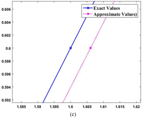
By employing the decomposition technique, the iterations of Eqs. (22) and (23) are calculated and displayed in Table 1 at z=1. These results are compared with the exact solutions, as shown in Figure 2, highlighting the method’s convergence towards the FDVFIDE. The FDVFIDE is solved using MATLAB R2015a.
Table 1. Comparison between exact and approximate solution
|
|
Exact Solution |
Approximate Solution |
||
|
T |
U(z) |
U(z) |
κ(z) |
κ(z) |
|
0 |
1 |
3 |
1.00735 |
3.00830 |
|
0.2 |
1.2 |
2.8 |
1.20584 |
2.80672 |
|
0.4 |
1.4 |
2.6 |
1.40595 |
2.60661 |
|
0.6 |
1.6 |
2.4 |
1.60606 |
2.40650 |
|
0.8 |
1.8 |
2.2 |
1.80617 |
2.2063 |
|
1.0 |
2 |
2 |
2.00628 |
2.00628 |
Figure 2. Convergences of exact and approximate method
The decomposition technique solves the given problem effectively based on the information provided. The approximate solutions converge to the exact solutions, suggesting that the method is accurate and stable.
The Adomian Decomposition Method (ADM) is a numerical technique for solving FDVFIDE. It's a reliable and efficient method that can handle complex equations with minimal computational effort. ADM has been shown to solve a wide range of FDVFIDE accurately, and its convergence properties have been studied in detail. ADM exhibits exceptional efficacy and efficiency in numerically resolving a comprehensive array of FDVFIDE.
The outcomes substantiate the convergence domain of the ADM series solution. An illustrative example, alongside the convergence theorem, underscores the method’s precision and effectiveness. The futuristic scope of the study is the convergence of different iterative techniques, and by increasing iteration, the convergence of the methods may be more efficient.
[1] Zadeh, L. (1975). The concept of a linguistic variable and its application to approximate reasoning. Information Science, 8: 199-249. https://doi.org/10.1016/0020-0255(75)90036-5
[2] Chang, S.S., Zadeh, L.A. (1972). On fuzzy mapping and control. IEEE Transactions on Systems, Man, and Cybernetics, (1): 30-34. https://doi.org/10.1109/TSMC.1972.5408553
[3] Kaleva, O. (1987). Fuzzy differential equation. Fuzzy Sets and Systems, 24: 301-317. https://doi.org/10.1016/0165-0114(87)90029-7
[4] Allahviranloo, T., Ahmady, N., Ahmady, E. (2007). Numerical solution of fuzzy differential equations by predictor-corrector method. Information Sciences, 177(7): 1633-1647. https://doi.org/10.1016/j.ins.2006.09.015
[5] Seikkala, S. (1987). On the fuzzy initial value problem. Fuzzy Set and System, 24: 319-330. https://doi.org/10.1016/0165-0114(87)90030-3
[6] Jafari, H., Saeidy, M., Baleanu, D. (2012). The variational iteration method for solving n-th order fuzzy differential equations. Central European Journal of Physics, 10(1): 76-85. https://doi.org/10.2478/s11534-011-0083-7
[7] Chalco-Cano, Y., Román-Flores, H. (2008). On new solutions of fuzzy differential equations. Chaos, Solitons & Fractals, 38(1): 112-119. https://doi.org/10.1016/j.chaos.2006.10.043
[8] Rasha H., Rawaa I., Alif (2023). The new Runge-Kutta Fehlberg method for the numerical solution of second-order fuzzy initial value problems. Mathematical Modelling of Engineering Problems, 10(4): 1409-1418. https://doi.org/10.18280/mmep.100436
[9] Allahviranloo, T., Abbasbandy, S., Hashemzehi, S. (2014). Approximating the solution of the linear and nonlinear fuzzy Volterra integro-differential equations using expansion method. Abstract and Applied Analysis. 2014: 1-8. https://doi.org/10.1155/2014/713892
[10] Al-Hayani, W., Younis, M.T. (2023). A numerical study for solving the systems of fuzzy Fredholm integral equations of the second kind using the Adomian Decomposition Method. Iraqi Journal of Science, 64(7): 4407-4430. https://doi.org/10.24996/ijs.2023.64.7.31
[11] Georgieva, A., Naydenova, I. (2022). Approximate solution of nonlinear Volterra-Fredholm fuzzy integral equations. AIP Conference Proceedings, 2505(1): 070002. https://doi.org/10.1063/5.0100646
[12] Osama M., Fadhel S., Mizal H., (2023). Using variational iteration method for solving linear fuzzy random ordinary differential equations. Mathematical Modelling of Engineering Problems, 10(4): 1457-1466. https://doi.org/10.18280/mmep.100442
[13] Amin, R., Ahmadian, A., Alreshidi, N.A., Gao, L., Salimi, M. (2021). Existence and computational results to Volterra-Fredholm integro-differential equations involving delay term. Computational and Applied Mathematics, 40: 1-18. https://doi.org/10.1007/s40314-021-01643-y
[14] Ziari, S., Bica, A.M., Ezzati, R. (2022). Successive approximations method for fuzzy Fredholm-Volterra Integral equations of the second kind. Advances in Fuzzy Integral and Differential Equations, 412: 209-228. https://doi.org/10.1007/978-3-030-73711-5_9
[15] Dubois, D., Prade, H. (1978). Operations on fuzzy numbers. International Journal of Systems Science, 9: 613-626. https://doi.org/10.1080/00207727808941724
[16] Narayanamoorthy, S., Yookesh, T.L. (2015). Approximate method for solving the linear fuzzy delay differential equations. Discrete Dynamics in Nature and Society, 2015: 1-9. https://doi.org/10.1155/2015/273830
[17] Nanda, S. (1989). On integration of fuzzy mappings. Fuzzy Sets and Systems, 32: 95-101. https://doi.org/10.1016/0165-0114(89)90090-0
[18] Zhou, Y. (2014). Basic Theory of Fractional Differential Equations. Singapore: World Scientific. 6.
[19] Hamoud, A.A., Ghadle, K. (2018). Homotopy analysis method for the first order fuzzy Volterra-Fredholm integro-differential equations. Indonesian Journal of Electrical Engineering and Computer Science, 11(3): 857-867.
[20] Adomain, G., Rach, R. (1983). Nonlinear stochastic differential-delay equations. Journal of Mathematical Analysis and Applications, 19(1): 94-101. http://doi.org/10.1016/0022-247X(83)90094-X
[21] Adomian, G. (1983). Stochastic Systems. Academic Press.
[22] Yookesh, T.L., Chithambarathanu, M., Kumar, E.B., Sekhar, P.S. (2021). Efficiency of iterative filtering method for solving Volterra fuzzy integral equations with a delay and material investigation. Materials Today: Proceedings, 47: 6101-6104. https://doi.org/10.1016/j.matpr.2021.05.025
[23] Amirali, I., Acar, H. (2024). Stability inequalities and numerical solution for neutral Volterra delay integro-differential equation. Journal of Computational and Applied Mathematics, 436: 115343. https://doi.org/10.1016/j.cam.2023.115343