Eskeziyaw Alemneh Mekonen![]() | Ayodeji Olalekan Salau*
| Ayodeji Olalekan Salau*![]() | Elisha Didam Markus
| Elisha Didam Markus![]() | Ermias Kassahun
| Ermias Kassahun![]() | Ting Tin Tin
| Ting Tin Tin![]()
© 2024 The authors. This article is published by IIETA and is licensed under the CC BY 4.0 license (http://creativecommons.org/licenses/by/4.0/).
OPEN ACCESS
An essential component of human survival is agriculture. Global human welfare is guaranteed by accurate and effective agricultural control. Conventional agricultural production regulation techniques are time-consuming, labor-intensive, and challenging, while pressing agricultural concerns continue to exist. Agricultural systems are complicated, multivariate, and unpredictable which can be difficult to control using classical control technologies. Model predictive control (MPC) techniques enhance spinning efficiency in a constrained temporal domain, which increases precision, and can provide very accurate control actions with moderate complexity. This paper presents a differential drive robot trajectory tracking approach to achieve minimum error using a mathematical model that controls kinematics and dynamics without coordinate transformation. By taking into account the physics of the engine and frame, a linear state-space dynamic model is developed. The dynamic and kinematic models are enhanced to yield one single state-space linear equation. Constraints on manipulated and controlled variables of the drive motors supply voltage are considered in the control design. To show the performance of the controller, different kinds of trajectories were implemented including circular and eight shaped using MATLAB Simulink software. The findings are examined critically and analytically. Furthermore, investigation was conducted to assess the controller's efficiency both in the presence and absence of unforeseen external disruption along with interior parameter change using a number of key performance measures, which include rise time, settling time, integral time absolute error (ITAE), integral time square error (ITSE), and integral absolute error (IAE). This analysis shows that the suggested MPC regulator is more predictable and flexible to changes in internal parameters and outside influences for the investigated system.
differential drive, dynamics, kinematics, model predictive control (MPC)
An essential component of human survival is agriculture. There are still difficult and urgent agricultural issues, and traditional methods of regulating agricultural output are labor- and time-intensive. Farming systems are intricate, multifaceted, and erratic. Classical control systems such as P, on/off, proportional integral (PI), and proportion-integration differentiation (PID) control are easy to implement, but they are not able to regulate time-delayed moving processes. Additionally, changing the controller takes a lot of effort and time [1].
Fuzzy logic (FL) control, hybrid models, non-mathematical extended scenarios, and predictable mathematical frameworks are also utilized in intelligent techniques such as artificial neural network (ANN) control. However, these techniques need thinking and picking up information from integrated or data-driven knowledge of experts [2].
Databases can be computationally costly, intricate, and difficult to use in real-world situations. Luckily, MPC performs better than older control and is simpler to employ than smart computing techniques. Excellent regulation precision can be achieved with MPC when the complexity level is appropriate. As such, precision agricultural yield meets the requirements for this sort of approach [3].
A particular kind of robot that has gained a lot of popularity is the differential drive mobile robot (DDMR), which is simple and easy to manage [4]. The following recent papers address robust and adaptive control of WMRs [5-7].
The most popular method for tracking a mobile robot's trajectory involves using sophisticated controllers to regulate its angular and linear velocities, and low-level controllers, such as PID controllers, to regulate its wheel speeds [8].
However, because of the limitations on inputs or naturally occurring states, it is challenging to achieve high performance in realistic implementations. The earlier mentioned works have not considered those limitations. Model predictive control (MPC) methods offer a simple solution for this. This is a significant problem for a WMR since the robot's position can be limited to fall inside a safe operating area. Control actions that respect actuator limits can be developed by taking input constraints into account.
Moreover, the dynamic system's coordinate transformations are no longer required, making the MPC's tuning parameter selection process more straightforward. MPC inherently generates a piecewise-continuous (non-smooth) control rule with respect to the nonholonomic properties of the WMR. Furthermore, the majority of DDMR-related article concentrates only on their kinematics models. But such a theory is only useful for low-speed, low-acceleration, light-load operations. Therefore, dynamic modeling must be considered if mobile robots are to work quickly and with large loads.
MPC is a system of control that uses optimization that utilizes the following elements: An objective function that articulates desired system behavior; a mathematical model of operational limits that must be satisfied; evaluations of the system's state at every step; and any data that is currently available about impending disturbances [9].
A WMR has a nonlinear model. Despite extensive development [10-12] the computational effort required for nonlinear model predictive control (NMPC) is significantly greater than that of the linear version. There is an online nonconvex nonlinear programming issue in NMPC. Since there are a numerous of selection factors, and obtaining a universal minimum is often not possible [13].
Employing the sequential linearization technique, one can generate a linear, variable in time system that can be solved using linear MPC. A range of trajectories are used to evaluate the performance of the suggested controller. The MPC controller performs well in trajectory tracking of the DDMR system when there are disruptions. In addition, an analysis is conducted to compare the controllers' responses using several performance indicators, such as integral squared error (ISE), integral absolute error (IAE), and steady state error.
This research's primary contribution is the construction of a linear time variant MPC for a pesticide spraying robot through the use of a successive linearization technique. The kinematics and dynamics of the robot are both augmented into a single state space model. By considering the mobile robot's complex kinematic and dynamic model, which takes the actuator and chassis dynamics into account, the accuracy of the model is significantly increased.
The other elements of the paper are organized as follows: Section 2 presents prior studies in the area of mobile robotics. Section 3 describes the DDWMR's nonlinear mathematical modeling, while Section 4 presents the control design of the MPC. Section 5 discusses the computer simulation results, and Section 6 provides the conclusion.
Ding et al. [3] proposed a nonlinear PID controller to regulate the DDMR's trajectory. While trajectory tracking control and stability are achieved with the proposed nonlinear PID controller, the precision is not as good as it may be. It should be noted that the nonlinear PID Controller finds widespread application in various industries due to its simplicity and easy of design. Nevertheless, employing a PID controller to attain satisfactory performance in nonlinear systems is challenging.
Lee et al. [14] compared PID controllers with fuzzy-PID controllers for DDMR path tracing. The authors conclude that the fuzzy-PID regulator is a good choice for path following control of DDMRs when compared to the PID controller. However, it should be noted that fuzzy-PID depends heavily on qualified expertise and that using fuzzy techniques does not necessarily guarantee reliability and robustness always ensured by the use of fuzzy approaches.
On the other hand, in the study conducted by Phuc [15], an adaptive fuzzy sliding mode control (AFSMC) was presented in for the purpose of controlling the trajectory surveillance of a robot system. The effectiveness of the suggested AFSMC was shown by the Simulink findings, which displayed good resilience and the ability to manage issues like parameter change and system disruption while also getting rid of chattering. It is important to note, although, that the sole focus of this work was on creating a controller, which is not the best option for path following control of DDMRs. Furthermore, actuator function was overlooked, which might have resulted in a decrease in system performance.
Similarly, Moudoud et al. [16] suggested an adaptive terminal integral sliding mode control (ATISMC) for a trajectory control of a wheeled mobile robot. It demonstrates quick convergence and robustness. But adding terminal sliding mode could make things more complicated, particularly for dynamic systems that are complicated like mobile robots.
As reported by Thay et al. [17], SMC was proposed as a controller for the trajectory tracking control of a mobile robot system. They compared the efficiency of a PID to that of SMC controller. The controller based on SMC outperformed the PID controller, according to the numerical simulation findings. However, due to undesirable control input behavior, the chattering in conventional SMC hindered its practical application.
Cáceres et al. [18] suggested an economical and periodic predictive controller. In order to maximize agricultural productivity, the controller seeks to determine the best irrigation method that minimizes energy and water usage while maintaining sufficient soil moisture levels for crops. To do this, a problem of optimization under constraints is formulated by the developed predictive controller using data on soil moisture at different depths. Nevertheless, the system was not integrated by the inventor with an autonomous robot. They solely take soil dynamics into account to maximize soil and water content.
The majority of the article that is currently available focuses on controller design and system modeling, primarily using the more basic kinematics model. However, using the kinematics model alone could not give the best velocity tracking in situations requiring fast motion or the transfer of large loads. In our approach, we handle this problem by considering both kinematic and dynamic models without the need of coordinate transformation. More over constraints are applied both on the inputs as well as outputs since performance cannot be improved in real system implementation due to limitations on actuators or naturally occurring states.
The paper provides three dynamic models of the robot. The kinematic model, the DC motor dynamics, and the chassis dynamics.
3.1 Dynamics of the mobile robot
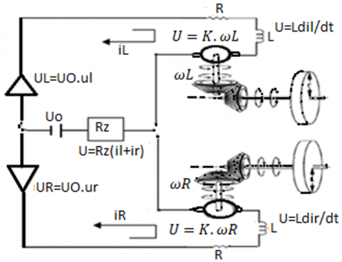
Based on Figure 1, it appears that the differential drive mobile robot is supported appropriately by a castor wheel and has two wheels connected to two DC series motors.
Figure 1. DC motor wiring of the robot
Kirchhoff's law, which applies to voltage balancing, and moment balancing can be used to determine the dynamics of a series DC motor. Apply Kirchhoff's voltage law from Figure 1 gives:
$\begin{gathered}R_a i_L(t)+R_z i_L(t)+i_R(t)+L_a \frac{d i_L(t)}{d t}=u_L V_a(t)- K_b \omega_L(t)\end{gathered}$ (1)
$\begin{gathered}R_a i_R(t)+R_z i_L(t)+i_R(t)+L_a \frac{d i_R(t)}{d t}=u_R V_a(t)- K_b \omega_R(t)\end{gathered}$ (2)
where, Kb is emf constant. ωR, ωL represent the right and left motor speeds.
The control voltages for the left and right motors are, respectively, uR, uL. In Figure 1, every other parameter is assigned.
Considering the balance of moments, we obtain:
$J_m \frac{d \omega_L}{d t}+K_r \omega_L+M_L=K_b i_L$ (3)
$J_m \frac{d \omega_R}{d t}+K_r \omega_R+M_R=K_b i_R$ (4)
where, Kr is the rotating resistance coefficient.
Table 1. DC motor parameters
|
Symbol |
Amount |
Unit |
Meaning |
|
R |
4 |
$\Omega$ |
Conductivity of windings |
|
L |
0.024 |
H |
Inductance of an engine |
|
K |
0.1 |
Kgm2s-2A-1 |
Motor constant |
|
Rz |
0.4 |
Ω |
Source resistance |
|
U0 |
24 |
$v$ |
Source voltage |
|
J |
0.0025 |
Kgm2 |
Inertia of rotor |
|
Kr |
0.00005 |
Kgm2.s-1 |
Coefficient of resistance |
|
PG |
25 |
- |
Gear box ration |
To verify the model's functionality, the motor parameters in Table 1 were used after several attempts using MATLAB simulation.
3.2 Chassis dynamics
The vector of angular velocity ωB, which is constant for all chassis locations, and the vector of linear velocity vB acting on a chassis reference point establish the dynamics of the chassis. The intersection of the axis connecting the wheels and the normal projection of the center of gravity is known as the chassis reference point B. Usually, it is positioned in the middle of the axis that connects the wheels and best explained by Sharma et al. [19].
Equilibrium of the loads and the current situation can be used to express the dynamics of the chassis. Applying the balance of forces yields Eq. (5). And the balance of moments yields Eq. (6) more explained by Dušek et al. [20].
$M_L+M_R-r_G K_v v_B-r_G m \frac{d v_B}{d t}=0$ (5)
$-M_L I_L+M_R I_R-K_\omega \omega_B-r_G J_B \frac{d \omega_B}{d t}=0$ (6)
where, Kω is the factor of opposition to turning and PG is the gear box transmission ratio.
The wheels' peripheral velocities (VL, VR) in relation to the angular velocity (ωB) and linear velocity (vB) at point B as:
$v_B=\frac{r_G}{I_L+I_R}\left(I_R \omega_L+I_L \omega_R\right)$ (7)
$\omega_B=\frac{r_G}{I_L+I_R}\left(-\omega_L+\omega_R\right)$ (8)
Input variables are the control signals, uL and uR that regulate the motors' supply voltages. By introducing some variables, Eqs. (1)-(8) can be reduced to a single state space representation.
$\dot{x}=A x+B u, y=C x+D u$ (9)
where, $x=\left[\begin{array}{c}i_L \\ i_R \\ \omega_L \\ \omega_R\end{array}\right], u=\left[\begin{array}{l}u_L \\ u_R\end{array}\right], C=\left[\begin{array}{c}v_B \\ \omega_B\end{array}\right], D=0$.
with constant matrices A, B and C as:
$A=\left[\begin{array}{cccc}-\left(\frac{R_a+R_z}{L_a}\right) & -\frac{R_z}{L a} & -\frac{k_b}{L a} & 0 \\ -\frac{R_z}{L a} & -\left(\frac{R_a+R_z}{L_a}\right) & -\frac{k_b}{L a} & 0 \\ k_b \frac{d_r+b_r L_L}{b_l d_r+b_r d_l} & k_b \frac{d_r-b_r L_R}{b_l d_r+b_r d_l} & -\frac{d_r a_l+b_r c_l}{b_l d_r+b_r d_l} & -\frac{d_r a_r-b_r c_r}{b_l d_r+b_r d_l} \\ k_b \frac{d_l-b_l L_L}{b_l d_r+b_r d_l} & \frac{d_l+b_l L_R}{b_l d_r+b_r d_l} & -\frac{d_l a_l-b_l c_l}{b_l d_r+b_r d_l} & -\frac{d_l a_r+b_l c_r}{b_l d_r+b_r d_l}\end{array}\right]$
$B=\left[\begin{array}{cc}\frac{v_a}{l_a} & 0 \\ 0 & \frac{v_a}{l_a} \\ 0 & 0 \\ 0 & 0\end{array}\right], C=\left[\begin{array}{cccc}0 & 0 & r_G \frac{L_R}{L_L+L_R} & r_G \frac{L_R}{L_L+L_R} \\ 0 & 0 & \frac{-r_G}{L_L+L_R} & \frac{r_G}{L_L+L_R}\end{array}\right]$
3.3 Kinematics of the mobile robot
Let α represent the robot's orientation, vB and ωB its linear and angular velocities, and (xB, yB) its global coordinates. Then the kinematic equations for the mobile robot with differential drive is given by Dušek et al. [21]:
$\frac{d x_B}{d t}=v_B \cos \alpha$ (10)
$\frac{d y_B}{d t}=v_B \sin \alpha$ (11)
$\frac{d \alpha}{d t}=\omega$ (12)
This can be expressed simply as:
$\frac{d x_B}{d t}=f\left(x_B, u_B\right)$ (13)
Eqs. (9)-(11), a non-linear model with regard to the reference robot, can be used to derive a linear model (see Figure 2). Calculating an error model in relation to a reference car yields a linear model. To achieve this, think about the reference vehicle that Eq. (12) also describes. Thus, its trajectory xr and ur are related by:
$\frac{d x_r}{d t}=f\left(x_r, u_r\right)$ (14)
Figure 2. Real robot and reference robot coordinate
The parameters for reference are [xr, yr, αr, ωr]. From Eqs. (9)-(11) the reference robot's angular velocity, orientation angle, and linear velocity may be obtained as:
$v_r=\sqrt{\left(\dot{x}_r\right)^2+\left(\dot{y}_r\right)^2}$ (15)
$\alpha_r=\arctan 2\left(\dot{y}_r, \dot{x}_r\right)$ (16)
$\omega_r=\dot{\alpha}_r=\frac{\dot{x}_r \ddot{y}_r-\dot{y}_r \ddot{x}_r}{\sqrt{\left(\dot{x}_r\right)^2+\left(\dot{y}_r\right)^2}}$ (17)
It follows that by extending the right side of Eqs. (9)-(11) in Taylor series around the point xr, ur and removing the high order terms gives:
$\dot{x}=f\left(x_r, u_r\right)+\frac{\partial f(x, u)}{\partial x}\left(x_B-x_r\right)+\frac{\partial f(x, u)}{\partial x}\left(u_B-u_r\right)$ (18)
Subtracting Eq. (17) from Eq. (13) and approximate the result by the forward difference gives a discrete (LTV) state-space model:
$\begin{gathered}\bar{Z}(k+1)=\bar{A}(k) \bar{Z}(k+1)+\bar{B}(k) \bar{u}(k) \bar{Y}(k)=\bar{C}(k) \bar{Z}(k)\end{gathered}$ (19)
A discrete error model is created by linearizing the kinematic model. Additionally, in order to supplement with a kinematic model, the dynamic model must be transformed into a discrete error-based model. The error model is the same as that of the above representation model since the dynamic model is linearly time invariant, but it needs to be discretized.
Model combination is more explained by Tilahun et al. [22].
$\begin{gathered}\dot{\bar{x}}_D(\mathrm{k}+1)=\bar{A}_D(k) \bar{x}_D(k)+\bar{B}_D(k) \bar{u}_D(k) \\ \bar{y}_D(k)=\bar{C}_D(k) \bar{x}_D(k)\end{gathered}$ (20)
A single mathematical representation with nine states (currents, wheel speeds, linear and angular velocities and coordinates), two control variables (motor voltage control input), and three outputs can be generated by augmenting the model, Eq. (19):
$\begin{gathered}\bar{Z}(k+1)=\bar{A}(k) \bar{Z}(k+1)+\bar{B}(k) \bar{u}(k) \\ \bar{Y}(k)=\bar{C}(k) \bar{Z}(k)\end{gathered}$ (21)
where,
$\bar{A}_{(K)}=\left[\begin{array}{cc}\bar{A}_{D(4 x 4)} & 0_{(4 x 5)} \\ \bar{C}_{D(2 x 4)} & 0_{(2 x 5)} \\ 0_{(3 x 4)} & \bar{B}_{K(3 x 2)} & \bar{A}_{K(3 x 3)}\end{array}\right]$,
$\bar{B}_{(K)}=\left[\begin{array}{c}\bar{B}_{D(4 x 2)} \\ 0_{(5 x 2)}\end{array}\right]$,
$\bar{C}_{(K)}=\left[\begin{array}{ll}0_{(3 x 6)} & \bar{C}_{K(3 x 3)}\end{array}\right]$,
$\bar{x}=\left[\begin{array}{lll}\bar{x}_D & \bar{u}_k & \bar{x}_k\end{array}\right], \bar{u}=\bar{u}_D$.
There is no control over this enlarged state space. We need a controlled model for the design model predictive to transport the states to any desired location. Over the aforementioned state space, a minimal realization is employed. Next, the MPC is designed using the robot's controllable model.
3.4 Disturbance Model affecting the DDWAR
The robot's goal is to carry an herbicide tanker and spring it to protect the vegetables from harm. When the robot starts working, the mass of the liquid occasionally decreases because the total weight of the machine equals the weight of the liquid in the tank plus the weight of the robot's body. The system's operation is altered by a decline in mass.
$m=m_h+m_b$ (22)
where, mh is mass of the herbicide and mb is mass of the body of the designed robot m is total mass of the robot. Figure 3 shows the flow of herbicide in very small pipe.
Figure 3. Flow of herbicide in very small pipe
The mass flow rate of the herbicide in the tank can be derived from the following equation.
$\begin{gathered}d m_h=\rho d V ; d V=A d x \\ d m_h=\rho A d x ; \frac{d m_h}{d t}=\frac{\rho A d x}{d t}=\rho A v\end{gathered}$ (23)
where, $\rho=$ density of herbicide, $\frac{d m_h}{d t}=$ mass flow rate, $v=$ velocity of herbicide flowing, $V=$ volume of herbicide flowing, $A=$ pipe cross sectional area.
Prior to incorporating the disturbance into the dynamic equation, it is crucial to ascertain which specific state it is impacting. From Eq. (9) from the state space model recall:
$\left[\begin{array}{l}d \omega_L / d t \\ d \omega_R / d t\end{array}\right]=\left[\begin{array}{cccc}k_b \frac{d_r+b_r L_L}{b_l d_r+b_r d_l} & k_b \frac{d_r-b_r L_R}{b_l d_r+b_r d_l} & \frac{d_r a_l+b_r c_l}{b_l d_r+b_r d_l} & \frac{-d_r a_r-b_r c_r}{b_l d_r+b_r * d_l} \\ k_b \frac{d_l-b_l L_L}{b_l d_r+b_r d_l} & \frac{d_l+b_l L_R}{b_l d_r+b_r d_l} & \frac{-d_l a_l-b_l c_l}{b_l d_r+b_r \mathrm{dl}} & \frac{-d_l a_r+b_l c_r}{b_l d_r+b_r d_l}\end{array}\right]\left[\begin{array}{c}i_L \\ i_R \\ \omega_L \\ \omega_R\end{array}\right]$ (24)
The total mass of the robot as the robot moves its mass decreases from time to time. This decrease in total mass does not affect the whole states or it does not affect the position and orientation of the designed robot. But as we already described in the state space model the variation of mass alters the angular velocity of the robot only. Therefore, due to variation in mass the above state space model can be modified into the following form:
$b_l=J_m+\left(m_h L_R \frac{r^2{ }_G}{L_L+L_R}\right)+m_b L_R \frac{r^2{ }_G}{L_L+L_R}$ (25)
$b_r=J_m+\left(m_h L_L \frac{r^2{ }_G}{L_L+L_R}\right)+m_b L_L \frac{r^2{ }_G}{L_L+L_R}$ (26)
Since $m_b$ is the robot's mass, it is constant over time. Only the parameters that contain the mass of the herbicide is considered to be known disturbance and its effect is well explained in the simulation part. So the known disturbances are only $m_h L_R \frac{r^2{ }_G}{L_L+L_R}$ and $m_h L_L \frac{r^2{ }_G}{L_L+L_R}$ is considered as a disturbance.
Optimizing process outcome forecasts across a range of foreseeable inputs is the primary goal of the model forecasting regulator. This is accomplished by applying an algorithm model over the forecast timeline, within a limited time frame. Following that, utilizing the new method data and a shifted horizon, the issue is solved once more at the next sampling time.
Internal Model Control (IMC) is the original source of evolution for the family of control systems known as Model Predictive Control (MPC). The processes sector widely employ MPC due to its ability to address limitations in an optimal way. Like the name suggests, maximum principle correction (MPC) relies on forecasts of the set point tracking conduct or refusal of disturbances derived from assessments of the two historical regulated and modified elements. A tuning method is utilized for each forecast to find the optimal source for the closed loop response that needs to satisfy predefined standards, such as the rate of output or profit function maximization [23].
MPC constitutes one of the widely prevalent techniques in the field of machine control. In actuality, it is one of the few cutting-edge control methods still offered by commercial industrial control systems today [24].
An optimization-based control technique that is ideal for meeting to forecast process outputs in the future within a given prediction horizon, it makes use of a process model, it, considering source and controlled variable restrictions as well as the process model, to identify the subsequent inputs for the process is called MPC [25]. MPC has been successful because it can tolerate MIMO control challenges naturally, handle limitations on the manipulated and controlled variables in a systematic way, is easy to tune, and is an entirely visible techniques relay on certain fundamental domains which permit for future extensions [26, 27].
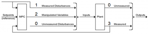
In essence, model forecast control computations are carried out at every sample interval, which the control designer may also specify. Current measurements and forecasts of future output values serve as the foundation for these computations. An MPC controller primarily performs two sorts of computations: control analysis, that contain process limitations and other explicitly given variables, and set-point calculations. An MPC controller's primary responsibility is to ascertain the best course of action for controlling the manipulated variable in order to track the system to its set-point [28, 29]. Figure 4 presents the MPC methodology.
Figure 4. MPC methodology
The model predictive controller optimizes a quadratic cost function to produce an ideal control sequence every time an observation interval is conducted. The event is subjected to the first control action in this sequence. The revised process inspections along with a changed perspective are used to solve the optimization issue once more at the subsequent sampling period.
The formulation of the cost function is contingent upon the control requirements.
The proposed forecasting regulator solves an optimization challenge to produce an ideal action series at every measurement period. The function of objective variables that needs to be reduced can be represented as a quadratic expression of the current state and the control components:
$\Phi_A=\sum_{i=1}^P \tilde{y}^T{ }_{(A+i \mid A)} W \tilde{Y}_{(A+i \mid A)}+\tilde{u}_{(A+i-1 \mid A)}^T L \tilde{u}_{(A+i-1 \mid A)}$ (27)
where, W≥0 and L>0 are the weighting function, and P is the forecasting horizon.
P, the prediction horizon, is a crucial factor to consider in Model Predictive Control. P must change inversely with sample time (Ts) if one decides to retain the prediction horizon duration (the product P*Ts ) constant. It is advised to start with the control interval duration (controller property Ts) when choosing sample time and to maintain it at that value while we adjust the other controller settings. We can edit Ts if the first selection was not the best one. We may then need to adjust other settings if we choose to do this.
Choose P so that $\mathrm{T} \cong \mathrm{P} * \mathrm{~T}_{\mathrm{s}}$ if the required closed-loop reaction time is T and the control interval is Ts.
The control horizon (m) is a crucial element in the design of an MPC controller. The number of manipulated variable (MV) motions to be optimized at each control interval k is known as the control horizon, or m. Select m in the interval between one and the forecasting horizon P. The default number is with m = 2. Every time, the control horizon (m<P) exceeds the prediction horizon.
Keep m<P for the following reasons: Smaller m indicates fewer variables to compute in the quadratic programming solved at each control interval, resulting in faster computations. In the event that the plant incorporates delays, m<p is crucial. Thirdly, m encourages the development of an internally stable controller, but it does not ensure one.
Figure 5. MPC design GUI
The MPC controller can be designed using the MPC app, using the command line using Simulink graphical tool.
The sample time and horizons can be changed while creating an MPC controller with the MPC app. This is done in the Tuning tab's horizon section. Figure 5 shows the MPC design GUI.
We can use state-space matrices, transfer functions, or a combination of the two with MPC Toolbox. Delays are another option; these are a typical occurrence in industrial facilities. A Simulink block for that environment is provided by the MPC Toolbox if we choose to model the plant using Simulink® graphical tools. It is simple to linearize a nonlinear Simulink plant, construct an MPC Controller block using the linearized model, and assess the linearized model's control over the nonlinear plant.
4.1 Constraints
The controller of a long-range predictive control must anticipate constraint violations and adjust control actions accordingly. The boundaries on the input are:
$\begin{array}{ll}\mathrm{u}_{\min } \leq \mathrm{u}(\mathrm{i}) \leq \mathrm{u}_{\max }, & \mathrm{i} \in\{\mathrm{k}, \mathrm{k}+\mathrm{N}-1\} \\ \mathrm{y}_{\min } \leq \mathrm{y}(\mathrm{i}) \leq \mathrm{y}_{\max }, & \mathrm{i} \in\{\mathrm{k}+1, \mathrm{k}+\mathrm{N}\}\end{array}$
Enter the constraint values in the constraints dialog box. Click constraints on the tuning tab of the MPC APP to set the properties of the controller constraint.
The next phase evaluates the efficiency of the proposed control strategy regardless of system perturbation and within variable modifications. We will take into account a constant state oversights, fluctuating replies, and efficiency indicators (like ITSE, IAE, ISE, and ITAE, which are carried out using MATLAB/Simulink, in order to determine the effectiveness of the proposed controller. Figure 6 depicts the default MPC controller structure, while Figure 7 shows a Simulink representation of the robotic vehicle with an MPC controller.
In this paper the three important parameters to use for the simulation are prediction horizon P=10, control horizon m=5 and a sample time of 0.1 s in the MATLAB software. The constraints to amplitude of the control variables are: vmin=-1.2m⁄s, vmax=1.2 m⁄s wmin=-1.2 rad⁄s, wmax=1.2 rad⁄s.
As previously mentioned, the MPC app allows one to import a plant from the MATLAB workspace or even a previously designed controller; the plant can be a linearized model that was obtained from a Simulink block diagram, or it can be a transfer function or state space model. Once a plant or controller has been imported, the user can set the properties of the input and output signals, including name, type of variable (manipulated, measured disturbance or unmeasured disturbance), description, physical units, and nominal value.
In this paper, the Simulink block was used to transmit information to the MPC controller. The following diagram shows the structure of the MPC toolbox.
In addition to other information, this window requests the number of MVs, measured outputs, and measured disturbances (for a feedforward technique). This initial section essentially checks if the block diagram's specified settings are correct and mostly describes the system. Once this tab has been completed, the controller parameters can be accessed.
Through following the above appropriate procedures for the design requirement of MPC the simulation results can be analyzed and discussed in the following section.
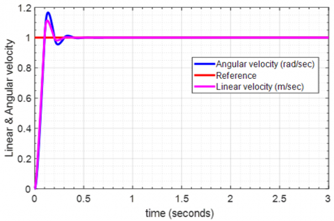
Figure 8 shows the simulation result of the linear and angular velocity. It is evident from Figure 6, that the control inputs fall within the bounds set by the constraints.
As observed from the simulation result, the linear and angular velocity can perfectly track the desired value of 1 m/s and 1 rad/sec respectively. The linear velocity achieves the desired velocity within a rise time of 0.0723, a settling time of 0.1892, and a peak time of 0.127 seconds. Likewise, the angular velocity achieves the desired velocity with a rise time of 0.0710, a settling time of 0.2797, and a peak time of 0.127 seconds. In Table 2, different error performances are given to show the controllers performance for linear and angular velocity. From the table, the average error (average IAE, average ISE, average ITSE and average ITAE) are 0.0069705, 0.0043785, 0.0001321 and 0.00040355 are presented respectively.
Figure 6. Default MPC controller structure
Figure 7. Simplified Simulink model of the robot with MPC controller
Figure 8. Angular and linear velocity of DDMR
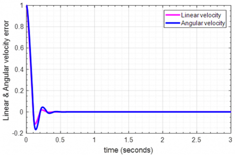
Figure 9. Angular and linear velocity error
Table 2. Analysis of the MPC controller
|
Controller Type |
State of Robot Dynamics |
IAE |
ISE |
ITSE |
ITAE |
|
Model Predictive Controller |
Linear Velocity |
0.006463 |
0.004172 |
0.0001182 |
0.0003351 |
|
Angular Velocity |
0.007478 |
0.004585 |
0.0001461 |
0.000472 |
Table 3. Performance of the controller at different error performance indices
|
Controller Type |
State of Robot Dynamics |
IAE |
ISE |
ITSE |
ITAE |
|
Model Predictive Controller |
ex |
0.01461 |
0.01151 |
0.0007337 |
0.00128 |
|
ey |
0.0201 |
0.01676 |
0.01516 |
0.002208 |
|
|
eθ |
0.01397 |
0.01086 |
0.0006601 |
0.001184 |
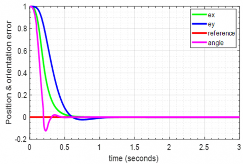
Figure 10. Position and orientation tracking error for MPC controller
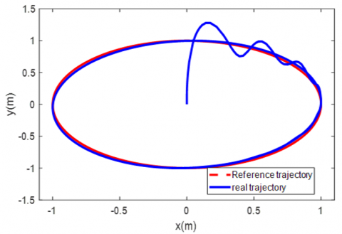
Figure 11. Circular trajectory tracking using MPC
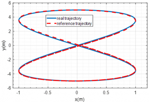
Figure 12. 8-shape trajectory tracking using MPC controller
As shown in Figure 9, the maximum error for angular velocity is 0.162 and linear velocity maximum error is 0.1. Since the objective of the robot is to move between crops for pesticide spraying purpose this error is relatively very small.
As presented in Table 3, the average error values which are (average IAE, average ISE, average ITSE and average ITAE) are respectively, 0.016226, 0.01304, 0.0055179, 0.001557 for the linear and angular velocity.
The mobile robot's trajectory tracking performance with model predictive controllers is shown in Figure 10. With an astonishingly quick settling time of 0.3646, rise time 0.1020, and peak time 0.2414 seconds, the x-position tracking error asymptotically approaches zero from an initial error of 1. likewise, the y position achieves the desired trajectory which is 1 m with a rise time of 0.1482, a settling time of 0.3048, and a peak time of 0.3724 with an overshoot of 1.6027. In addition, the orientation angle alpha achieves the desired value with rise time of 0.1013, settling time of 0.3643, peak time of 0.2371 seconds.
To evaluate this research with prior research, the primary evaluation variables, such as equilibrium error, settlement time, location measuring error, and direction tracking error, had been acquired.
As shown in Figure 10, the tracking errors (ey and e$\theta$) reach at maximum value of 0.0825 and 0.15, before reduced to zero with a settling time of 0.3048 and 0.3643 respectively.
In addition to tracking, it is better to show other simulations to check the validity of the designed robot performance. We have also included circular and eight shaped trajectories. The fundamental routine for the mobile machine is chosen to be for circular (xref=cos(2*t), yref=sin(2*t)) & 8-shaped (xref=cos(t), yref=sin(2*t)) in order to evaluate the tracking capabilities of the suggested controller in the simulation. Trajectory tracking simulation time for a circular reference trajectory is 10 seconds, assuming the robot starts at origin (0, 0) and the reference trajectory starts at point (1, 0).
The system's performance response for following the circular reference trajectory for the MPC controller is indicated in Figure 11. From the figures, we can see that, with higher performance, the actual trajectory follows or tracks the reference trajectory from the starting point to the end of the simulation period allocated.
In addition, an 8-shape trajectory is generated and uploaded to the mobile robot system in order to keep track of its position in an appropriate way. The tracking results are shown in Figure 12.
5.1 Disturbance rejection and sensitivity to internal parameter variation
As we explained earlier the mass change of the robot does not affect the position of the robot, the orientation of the robot and the linear and angular velocity of the robot. to check the validity of disturbance rejection capability of the controller we modify the parameter of the robot which is mass change of the robot and a disturbance is added to the block and we will explain its effect in detail.
In parameter variation we change the variation of mass of the robot which is 0.5kg and the rest of the parameters are unchanged. This is because the objective of the designed robot is to carry an herbicide tanker and its mass changes constantly as the robot moves. As an external disturbance we apply a unit step signal at a simulation of 2 seconds.
The linear and angular velocity does not be affected by mass change of the robot. but due to the application of external disturbance at a time of 2 seconds the error performance indices parameters slightly varied but this variation is not significant. This is graphically shown in Figure 13.
The accuracy and efficacy of the controllers against random external disturbances were assessed using a variety of performance index measures, including integral square error (ISE), integral absolute error (IAE), integral time square error (ITSE), and integral time absolute error (ITAE).
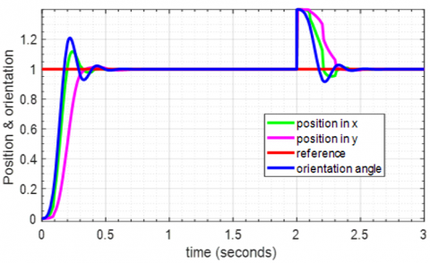
The results of the experiment demonstrate that, regardless of inner parameter modifications or external disruptions, the planned controller operates effectively all the time. The average error performance measures (ISE, IAE, ITSE, and ITAE) only encounters a slight modification which is (0.004555, 0.008357, 0.0004868, and 0.003301, respectively). However, the time domain specification parameters are still the same. The settling time for linear motion is 0.1892, whereas for angular velocity it is 0.2797. This indicates how effectively the proposed controller model forecasting regulator (MPC) can manage changes in its internal parameters and function even when external influences are present, resulting in the lowest amount of tracking error. The performance index of the controller for various errors shows that, for ITAE, the maximum value of 0.008602 is obtained along Y with an external disturbance; for IAE, ITSE, and ISE, the corresponding values are 0.02426, 0.002927, and 0.01747. The IAE achieves the highest value (0.00282) along with θ and external disturbance, whereas ISE, ITSE, and ITAE achieve 0.01129, 0.001555, and 0.007008. According to the results, the biggest error was obtained along the Y-axis with disturbance (0.01081) using ITAE, whereas the least error was reached along θ with external disturbance (0.001555) using ITSE. This is shown in Figure 14.
Figure 13. Linear & angular velocity with disturbance
Figure 14. Disturbance rejection using MPC controller
The variation in mass still does not affect the performance of the controller but due to external added disturbance signal the different measurement error indices are slightly modified but not due to internal parameter variation. Agricultural robots encounter a number of disturbances. This could be due to parameter variation, due to external disturbances, due to soil content, due to sloppy and sticky conditions and so on. The designed robot is for pesticide spraying purpose. Since the mass of herbicide is decrease from time to time this is considered as a disturbance and this effect is clearly shown in the simulation.
Better results have been found using the linear model predictive controller in comparison to trajectory tracking based studies. The results show that we can achieve a minimal rise time of 0.1013 and faster settling time of 0.3048 seconds using the model predictive controller.
From the obtained result we can say that the proposed model predictive controller has a better disturbance rejection capability and internal parameter variation. This is one more advantage of using model predictive controller.in section one we have explained the unique advantage of model predictive controller which is handling of constraints. Due to naturally occurring states and actuator limitations it is difficult to implement the real system. This disadvantage can be easily reversed by using model predictive controller. The capacity of MPC to conform to constraints whether they are simple limitations on states or controls or more complicated ones sets it apart from other advanced control systems. This is especially important when the real system is operating close to its limits or in potentially collision-prone situations, such autonomous robotics. Not only does MPC guarantee safety and operational efficiency, but it also improves predictability and dependability in contexts that are uncertain and dynamic by directly integrating constraints into the control issue. By adjusting the limitations or the parameters of the cost function, MPC is also readily adjusted and changed.
However, since having an exact model of the system is not always attainable, particularly for non-linear systems, MPC requires an accurate model of the system in order to provide suitable control inputs. This may not always be the case. Large unmodeled external disturbances have the potential to seriously impair the MPC controller's performance because they are not included in the system model.
In this paper, we proposed a differential type machine model that considers the dynamics of the actuator and chassis in addition to the impacts of kinematics. The model was validated by simulations involving real-time scenarios. A range of assessment criteria were utilized for performance comparison, such as equilibrium error and time domain specification parameters as well as error performance indices (ISE, IAE, ITSE, and ITAE).
The suggested model predictive controller demonstrates a superior ability to improve trajectory tracking performance and robustness, as evidenced by the outcome results utilizing both circular and 8-shaped inputs, showing that tracking performance remains constant even in the face of uncertainty. Moreover, the suggested controller demonstrates flexibility with respect to different reference paths, making it an efficient choice for dynamic systems. It outperforms typical controllers in uncertain settings and generally has extraordinary robustness in handling uncertainty. These results confirm the suggested controller's viability and suitability for use in real-world control systems.
In this work, MPC is suggested for motion control of the differentially driven wheeled agricultural pesticide robot. State space representation was used to describe the model of the robot, and an augmented model was obtained and used in the simulation part. Error minimization is used as a performance index for the controller. The constraint only applies to the manipulated and controlled variables, but in subsequent studies, wheel speeds will also be subject to limits, and it is better to include slopy and sticky area of land and better to include the resistance effect of soil in the irrigation.
[1] Qu, J., Zhang, Z., Qin, Z., Guo, K., Li, D. (2024). Applications of autonomous navigation technologies for unmanned agricultural tractors: A review. Machines, 12(4): 218. https://doi.org/10.3390/machines12040218
[2] Bumroongsri, P., Kheawhom, S. (2014). Off-line robust constrained MPC for linear time-varying systems with persistent disturbances. Mathematical Problems in Engineering, 2014(1): 936093. https://doi.org/10.1155/2014/936093
[3] Ding, Y., Wang, L., Li, Y., Li, D. (2018). Model predictive control and its application in agriculture: A review. Computers and Electronics in Agriculture, 151: 104-117. https://doi.org/10.1016/j.compag.2018.06.004
[4] Leena, N., Saju, K.K. (2016). Modelling and trajectory tracking of wheeled mobile robots. Procedia Technology, 24: 538-545. https://doi.org/10.1016/j.protcy.2016.05.094
[5] Belay, A., Salau, A.O., Kassahun, H.E., Eneh, J.N. (2024). Stator flux estimation and hybrid sliding mode torque control of an induction motor. International Journal of System Assurance Engineering and Management, 15: 2541-2553. https://doi.org/10.1007/s13198-024-02275-1
[6] Zangina, U., Buyamin, S., Abidin, M.S.Z., Azimi, M.S., Hasan, H.S. (2020). Non-linear PID controller for trajectory tracking of a differential drive mobile robot. Journal of Mechanical Engineering Research and Developments, 43(7): 255-270.
[7] Bosera, A.S., Salau, A.O., Yadessa, A.G., Jembere, K.A. (2022). Finite time trajectory tracking of a mobile robot using cascaded terminal sliding mode control under the presence of random Gaussian disturbance. In International Conference on Advances of Science and Technology, pp. 63-78. https://doi.org/10.1007/978-3-031-28725-1_5
[8] Maurović, I., Baotić, M., Petrović, I. (2011). Explicit model predictive control for trajectory tracking with mobile robots. In 2011 IEEE/ASME International Conference on Advanced Intelligent Mechatronics (AIM), pp. 712-717. https://doi.org/10.1109/AIM.2011.6027140
[9] Negenborn, R.R., Maestre, J.M. (2014). Distributed model predictive control: An overview and roadmap of future research opportunities. IEEE Control Systems Magazine, 34(4): 87-97. https://doi.org/10.1109/MCS.2014.2320397
[10] Zhou, H., Güvenç, L., Liu, Z. (2017). Design and evaluation of path following controller based on MPC for autonomous vehicle. In 2017 36th Chinese Control Conference (CCC), pp. 9934-9939. https://doi.org/10.23919/ChiCC.2017.8028942
[11] Utstumo, T., Berge, T.W., Gravdahl, J.T. (2015). Non-linear model predictive control for constrained robot navigation in row crops. In 2015 IEEE International Conference on Industrial Technology (ICIT), pp. 357-362. https://doi.org/10.1109/ICIT.2015.7125124
[12] Bouzoualegh, S., Guechi, E.H., Kelaiaia, R. (2018). Model predictive control of a differential-drive mobile robot. Acta Universitatis Sapientiae, Electrical and Mechanical Engineering, 10(1): 20-41. https://doi.org/10.2478/auseme-2018-0002
[13] Henson, M.A. (1998). Nonlinear model predictive control: Current status and future directions. Computers & Chemical Engineering, 23(2): 187-202. https://doi.org/10.1016/S0098-1354(98)00260-9
[14] Lee, K., Im, D.Y., Kwak, B., Ryoo, Y.J. (2018). Design of fuzzy-PID controller for path tracking of mobile robot with differential drive. International Journal of Fuzzy Logic and Intelligent Systems, 18(3): 220-228. https://doi.org/10.5391/IJFIS.2018.18.3.220
[15] Phuc, P.T., Tho, T.P., Hai, N.D.X., Thinh, N.T. (2021). Design of adaptive fuzzy sliding mode controller for mobile robot. International Journal of Mechanical Engineering and Robotics Research, 10(2): 54-59.
[16] Moudoud, B., Aissaoui, H., Diany, M. (2023). Adaptive integral-type terminal sliding mode control: Application to trajectory tracking for mobile robot. International Journal of Adaptive Control and Signal Processing, 37(3): 603-616. https://doi.org/10.1002/acs.3540
[17] Thay, A.O., Basri, M.A.M., Subha, N.A.M., Shamsudin, M.A., Sahlan, S. (2018). Sliding mode controller for trajectory tracking control of autonomous mobile robot. ELEKTRIKA-Journal of Electrical Engineering, 17(1): 28-33. https://doi.org/10.11113/elektrika.v17n1.27
[18] Cáceres, G., Millán, P., Pereira, M., Lozano, D. (2021). Smart farm irrigation: Model predictive control for economic optimal irrigation in agriculture. Agronomy, 11(9): 1810. https://doi.org/10.3390/agronomy11091810
[19] Sharma, K.R., Honc, D., Dusek, F. (2016). Predictive control of differential drive mobile robot considering dynamics and kinematics. In ECMS, pp. 354-360.
[20] Dušek, F., Honc, D., Rozsíval, P. (2011). Mathematical model of differentially steered mobile robot. In 18th International Conference on Process Control, Tatranská Lomnica, Slovakia, pp. 221-229.
[21] Dušek, F., Honc, D., Rozsíval, P. (2011). Mathematical model of differentially steered mobile robot. In 18th International Conference on Process Control, Tatranská Lomnica, Slovakia, pp. 221-229.
[22] Tilahun, A.A., Desta, T.W., Salau, A.O., Negash, L. (2023). Design of an adaptive fuzzy sliding mode control with neuro-fuzzy system for control of a differential drive wheeled mobile robot. Cogent Engineering, 10(2): 2276517. https://doi.org/10.1080/23311916.2023.2276517
[23] Ashagrie, A., Salau, A.O., Weldcherkos, T. (2021). Modeling and control of a 3-DOF articulated robotic manipulator using self-tuning fuzzy sliding mode controller. Cogent Engineering, 8(1): 1950105. https://doi.org/10.1080/23311916.2021.1950105
[24] Álvarez, A., Ridao, M.A., Ramirez, D.R., Sánchez, L. (2013). Constrained predictive control of an irrigation canal. Journal of Irrigation and Drainage Engineering, 139(10): 841-854. https://doi.org/10.1061/(ASCE)IR.1943-4774.0000619
[25] Breckpot, M., Agudelo, O.M., De Moor, B. (2013). Flood control with model predictive control for river systems with water reservoirs. Journal of Irrigation and Drainage Engineering, 139(7): 532-541. https://doi.org/10.1061/(ASCE)IR.1943-4774.0000577
[26] Bosera, A.S., Salau, A.O., Yadessa, A.G., Jembere, K.A. (2022). Finite time trajectory tracking of a mobile robot using cascaded terminal sliding mode control under the presence of random Gaussian disturbance. In International Conference on Advances of Science and Technology, pp. 63-78. https://doi.org/10.1007/978-3-031-28725-1_5
[27] Mayne, D.Q., Rawlings, J.B., Rao, C.V., Scokaert, P.O. (2000). Constrained model predictive control: Stability and optimality. Automatica, 36(6): 789-814. https://doi.org/10.1016/S0005-1098(99)00214-9
[28] Schwenzer, M., Ay, M., Bergs, T., Abel, D. (2021). Review on model predictive control: An engineering perspective. International Journal of Advanced Manufacturing Technology, 117(5): 1327-1349. https://doi.org/10.1007/s00170-021-07682-3
[29] Rezaee, A. (2017). Model predictive controller for mobile robot. Transactions on Environment and Electrical Engineering, 2: 17.