Mamidi Naveen Babu![]() | Pradyumna Kumar Dhal*
| Pradyumna Kumar Dhal*![]()
© 2024 The authors. This article is published by IIETA and is licensed under the CC BY 4.0 license (http://creativecommons.org/licenses/by/4.0/).
OPEN ACCESS
The crow search algorithm (CSA) was developed to optimize swarm intelligence by modeling crows' clever food concealment and retrieval. Simple structure, few tuning parameters, and easy implementation characterize the method. The crow search technique is used to frame an imbalanced radial distribution network in this research. This study aims to decrease power losses in uneven distribution networks via design. CSA strategies like power flow and DG placement decrease losses. A load-flow method for three-phase unbalanced radial distribution networks may easily incorporate these solutions into present networks. This approach optimizes network phase balance and conductor sizes. Planning goals include reducing total complex power imbalance, power loss, and average voltage drop. The thermal limit of each line and the minimum and maximum voltage limitations for each bus voltage confine the optimization. A three-phase forward–backward sweep load flow technique was developed to calculate these objective functions. The framing approach was evaluated on unbalanced radial distribution networks with 19 and IEEE 25 buses to determine its efficiency. Power loss and voltage drop are significantly reduced by optimizing phase balance and conductor sizes together. CSA outperformed and was more consistent than several meta-heuristic algorithms studied in this work.
unbalanced system, distributed generation, crow search algorithm, IEEE 19 & 25 buses
Phase loading disrupts dispersion. Distribution lines have a larger mutual inductance than transmission lines because they are seldom transposed, unbalancing them. These generate three-phase branch/line current inequality. Thus, neutral current and power loss grow. Phase unbalancing may trip relays. Phase balancing improves voltage profile and power quality. It increases distribution line capacity. Many academics and operators care about distribution system optimization. Distribution and size of reactive power sources and DG allocation are using metaheuristic optimization. Can-based, derivative-free, discrete objective function algorithms have been developed recently. No strategy is suitable for all optimization scenarios, says the no-free lunch hypothesis. Tuning parameters, local minimum escape, convergence rate, and reliability differ across these methods. These methods use random search, random starting population, exploration-exploitation phases to find new candidate solutions, and uncertain stopping criteria. Inefficient components waste power in distribution networks. Weather, overloading, etc. malfunction. Inefficiency and failure waste energy. System operators retrieve loads individually. Rethink feeders. The feeder reset turns switches on and off to change network design to electricity distribution. Adjustments to feeders minimize power loss, balance network load, optimize voltage outline, and increase reliability and efficiency [1, 2].
Restructuring distribution networks reduces losses and branch overload. Reasons to restructure. Using restructure, load balancing avoids converter and queue overflow. Resetting may reduce network power loss under certain loads [3]. After restoring non-error sections and deleting error sites from active sinners, emergency rehabilitation is achievable. Healthy networks can restructure. A functional network is simpler to redesign owing to power and communication. System imbalance hinders reorganization due to classifications. All three phases must be considered in power distribution systems. Reorganizing distribution networks cuts costs. Heuristic reduction, imitation, and genetic process reduce losses [4-7]. CSA, Askarzadeh's 2016 swarm intelligence optimization method, is simple, has few control parameters, and is easy to apply. Central power plants generate hundreds of MW to several GW [8]. Power plants are generally unprofitable due to dwindling fuel reserves, increased fuel costs, and stricter environmental regulations [9]. Wind and solar energy are cheaper and simpler. Small power plants connected to the distribution network near end consumers are termed "embedded" or "distributed" generation [10]. Radial distribution network capacitor placements and sizes are determined in two steps in this study. Choosing the best capacitor placements starts with two loss sensitivity indices (LSIs). In the second stage, ant colony optimization is utilized to arrange and size capacitors to optimize energy loss and cost while fulfilling system requirements [11].
Electrical distribution networks use shunt capacitors to adjust reactive power. These methods reduce feeder capacity, voltage shape, and loss. Distribution network capacitor size and location need combinatorial optimization. The goal function should reduce power losses and capacitor installation costs under operational limitations [12].
Due to delayed expansion, high load growth, and increased distribution generation (DG) penetration, distribution system functioning requires voltage stability. Three-phase unbalanced distribution systems were analyzed for voltage stability using modal analysis [13]. The effects of renewable energy output unpredictability on scattered networks are studied using a non-linear three-phase maximum loadability model. The cumulate-based probabilistic evaluation of static voltage stability for distributed networks incorporates wind power generation and load forecasting variation. Studying neighboring wind farm correlations. Three-phase unbalanced power network maximum load increment models are solved using enhanced self-adaptive particle swarm technique. Cornish–Fisher and Gram–Charlier expansions construct random variable probability distributions [14].
This paper proposes a robust voltage control optimisation approach for unbalanced radial distribution systems with load and distributed generation uncertainty. To solve mixed-integer nonlinear programming (MINLP), a two-stage technique was developed. The recommended method's resilience was tested using Monte Carlo simulations [15]. Unbalanced DN voltage control solutions are supported by literature. Our method for the compulsory voltage control auxiliary service avoids active power production curtailments and regulates with low reactive power. The IEEE 13-bus distribution system showed encouraging results for the suggested control [16]. This study optimises multiphased unbalanced distribution network distributed generator (DGS) allocation using particle swarm optimisation (PSO). PSO was built in MATLAB using Open DSS in a co-simulation environment to solve unbalanced three-phase optimal power flow (TOPF) and find the best location and size of different distributed generators [17].
The study covers all planning technology advances, including optimization models and solution methods. This cutting-edge survey helps future researchers and engineers’ plan. The first two planning models in a three-level categorization framework are without and with reliability concerns. Subdivisions grow trees. This category tree concludes with planning and solving methods [18].
Power distribution feeders are imbalanced due to unbalanced loads. Unbalanced feeders affect three-phase devices. Balance feeders. Phase shifting balances feeder phases [19].
A mesh-based alternative replaced nodes, graph theory, and typical injection techniques. To demonstrate their superior skill. Most alternative methods for enhancing power system generation and growing power requirements include distribution network reconfiguration and optimal distributed generator. Optimisation maximises cost reductions after radial distribution network reconfiguration. Both algorithms perform better together [20]. This research introduces a new method for optimizing distribution network topology modification and DG installation. This technique uses GA, PSO, and BWO optimization methods. This study optimizes DG placement to decrease losses in a balanced radial distribution system [21]. Unbalanced distribution systems calculate load flows forward and backward. The best string is found by randomly exchanging information via crossover and mutation to imitate natural selection [22]. This approach uses the loop frame of reference instead of the bus frame. The reference frame for this loop is a simple direct iterative impedance technique. The approach also uses graph theory and injection current [23]. This study uses a simple three-phase load flow technique to fix an unbalanced three-phase radial distribution system (RDS). The issue is solved using a simple algebraic recursive voltage value equation using vector data. Simple circuit theory ideas underpin the method. The mathematical model now accounts for phase interaction. The report shows the imbalanced RDS results from testing the recommended approach on many unbalanced distribution networks [24]. A fast power flow decoupling approach is given by Zimmerman and Chiang [25]. Layering laterals instead of buses reduces the issue. Lateral variables are more efficient than bus variables, but they might become troublesome when the network design changes regularly, like in distribution systems due to switching activities.
We provide several distribution automation strategies and discuss URDS unbalanced distribution load flow studies in this work. Our method for determining the 3-ph load flow of an unbalanced radial distribution network is to thoroughly model its components. One recursive algebraic equation accounts for receiving voltage. This method uses static load models since load voltage changes per system.
Many load flows for BRDS analysis cannot be utilized for URDS. It is difficult to choose a load flow that works for both BRDS and URDS.
Research into statistical performance comparisons of metaheuristics is promising for refining algorithms and designing unequal distribution systems. These processes are essential to planning and design, especially in DG-integrated systems. Finding the ideal mix analytically takes longer. Thus, determining the ideal switch combination requires arithmetic. Loop matrix for optimum dg placement determines the best number of combinations.
The remainder of this work is divided: Unbalanced distribution load flow is shown in section 2; suggested CSA is in section 3. Section 4 presents simulation findings for different test situations, and section 5 concludes.
Electricity flow must be monitored in any power system. Power drift analysis for the suspension of three phases (3-ph) of the electrical device is necessary for proper planning due to energy structure disparities induced by continuous transmission lines and load discrepancies [22]. Watt and wattle power fluxes in each feeder are the main focus of this section [24]. Traditional static nation evaluation using energy structures has used three-dimensional measurements and switching gearbox traces to estimate loads. Radial distribution networks sometimes do not. Thus, the profile shows three uneven segment networks, making single-phase evaluation methods obsolete. Energy imbalance may be addressed by considering segment size and connection equipment quality. Thus, power flow solutions are uneven, necessitating a unique network correction technique [26, 27]. The admittance matrix of buses i and j in Eq. (1) is a 6×6 matrix with series impedance Z and shunt admittance Y.
$Y_{i j}=\left[\begin{array}{cc}Z^{-1}+\frac{1}{2} Y & -Z^{-1} \\ -Z^{-1} & Z^{-1}+\frac{1}{2} Y\end{array}\right]$ (1)
Voltages and currents of 3×1 vectors Vi, Iiand Ij.
$\left\lfloor\frac{I_i}{I_j}\right\rfloor=Y_{i j}\left[\frac{\mathrm{V}_{\mathrm{i}}}{\mathrm{V}_{\mathrm{j}}}\right]$ (2)
For a network has n nodes, the node voltage vector (Vbus) and node current vector (Ibus) are obtained as:
$V_{\mathrm{bus}}=\left[V_1^a, V_1^b, V_1^c, V_2^a, V_2^b, V_2^c, \ldots, V_n^a, V_n^b, V_n^c\right]^T$ (3)
where, Vip is complex voltage and Iip is current of phase p in bus i (injected current).
$\mathrm{I}_{\text {bus }}=Y_{\text {bus }} V_{\text {bus }}$ (4)
where, $Y_{\text {bus }}=\left[Y_{i j}^{p m}\right]$ complex 3n×3n matrix, its function links voltage Vjm to the current Iip.
Rewriting Eq. (4) will become Eq. (5).
$I_i^p=\sum_{j=1}^n \sum_{m=a}^c Y_{i j}^{p m} V_j^m$ (5)
The watt and wattles powers are in Eqs. (7) and (8).
$S_i^p=P_i^p+Q_i^p$ (6)
$\begin{gathered}P_i^p=\left|V_i^p\right| \sum_{j=1}^n \sum_{m=a}^c\left|V_j^m\right|\left[G_{i j}^{p m} \cos \theta_{i j}^{p m}\right. \left.+B_{i j}^{p m} \sin \theta_{i j}^{p m}\right]\end{gathered}$ (7)
$Q_i^p=\left|V_i^p\right| \sum_{j=1}^n \Sigma_{m=a}^c\left|V_j^m\right|\left[G_{i j}^{p m} \sin \theta_{i j}^{p m}-B_{i j}^{p m} \cos \theta_{i j}^{p m}\right]$ (8)
$Y_{i j}^{p m}=G_{i j}^{p m}+j B_{i j}^{p m}$ (9)
$\theta_{i j}^{p m}=\theta_i^p-\theta_j^m$ (10)
The real and reactive power losses in branch pq is obtained as:
$\left[\begin{array}{l}L S_{p q}^a \\ L S_{p q}^b \\ L S_{p q}^c\end{array}\right]=\left[\begin{array}{l}L P_{p q}^a+j L Q_{p q}^a \\ L P_{p q}^b+j L Q_{p q}^b \\ L P_{p q}^c+j L Q_{p q}^c\end{array}\right]=\left[\begin{array}{l}V_p^a \cdot\left(I_{p q}^a\right)^*-V_q^a \cdot\left(I_{q p}^a\right)^* \\ V_p^b \cdot\left(I_{p q}^b\right)^*-V_q^b \cdot\left(I_{q p}^b\right)^* \\ V_p^c \cdot\left(I_{p q}^c\right)^*-V_q^c \cdot\left(I_{q p}^c\right)^*\end{array}\right]$ (11)
2.1 Problem formulation
The goal function in 3-ph distribution network is:
MinimizeTPL $=\sum_{p q=1}^{b r} L P_{p q}^{a b c}=\sum_{p q=1}^{b r} I_{p q}^{a b c T} \operatorname{Re}_{p q}^{a b c} I_{p q}^{a b c}$ (12)
Subjected to
Voltage, current and source constraints are Eqs. (13)-(15) respectively:
$V_q^{\min } \leq V_q \leq V_q^{\max }$ (13)
$I_{p q} \leq I_{p q}^{\max }$ (14)
$P_{p q} \leq P_{p q}^{\max }, \quad Q_{p q} \leq Q_{p q}^{\max }$ (15)
2.2 Distribution load flow using DG model
In uneven distribution networks, DGs are introduced. A piece of an unbalanced distribution network sample line and a connection configuration for three DGs of different kW ratings linked to bus j are shown in Figure 1.
Figure 1. Connection diagram of DGs in a sample unbalanced distribution system
The a, b, and c have different impedances. To integrate the DG model, bus i's active power demand must be adjusted. DG ratings remain valuable. To add the DG model, modify the active power demand at bus i, where a DG unit is located.
$P_{D i p}^{D G}=P_{D i p}^{b j e s}-P_{i p}^{D G}$ (16)
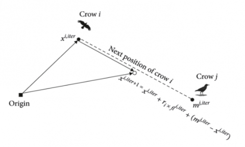
The newly developed crow search algorithm is inspired by how crows remember cache sites. Crows are extremely greedy and will band together to steal food after the owner leaves. Crows defend themselves in several ways [3, 28]. CSA works in d-dimensional space with NN crows, like prior metaheuristic algorithms. Rooster perches represent alternative solutions to the dilemma. Figure 2 and Figure 3 illustrate crow i's position at iteration iter.
$x^{i, \text { iter }}=\left[x_1^{i, \text { iter }}, x_2^{i, \text { iter }}, \ldots, x_d^{i, \text { iter }}\right]$
Crow number is i, iteration number iter. Crows should remember caches. The Crow i cache at iteration no is mmii,iii. Best crow yet. Crows remember their greatest moments. Crows want better food. Crow follows the other crows to the cache and snatches food after the owner departs. Consider i and jj crows. Crow j will visit cache mmjj,iii at iteration no. Crow i eats with j. There are two options:
CSA's fundamental process:
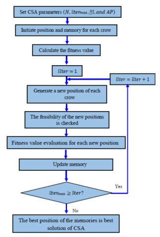
Step 1: Initialising CSA parameters: population size (n), maximum iteration number (Maxsize), flight step size (fl), and awareness probability (AP).
Figure 2. Schematic diagram for updating the position of crow i, when fl<1
Figure 3. Schematic diagram for updating the position of crow i, when fl>1
Step 2: Initialising each crow and memory matrix. n crows are created in the search space of d − dimension, and each crow xi (Xi,1, Xi,2, ..., Xi,d) indicates a plausible issue solution. The beginning population has no experience, hence the memory matrix is the initial position.
Step 3: Fitness function-based crow quality evaluation.
Step 4: Relocating each crow in the d − dimensional search space. If crow i randomly follows a crow, such as crow j, to discover its concealed food, its location update may be classified into two situations:
Case 1: Crow jj doesn't see crow i following it. Crow i will take food from crow jj's stash.
Case 2: Crow jj observes crow i following it. In this situation, crow jj would fool crow i by randomly travelling to another search area to safeguard its thieving hiding location. Case 1 and 2 expression:
$x^{i, \text { iter }+1}=\left\{\begin{array}{cc}x^{i, \text { iter }}+r_i \times f l^{i, \text { iter }} \times\left(m^{j, \text { iter }}-x^{i, \text { iter }}\right), & r_j \geq A P^{j, \text { iter }} \\ \text { a random number, } & \text { otherwise }\end{array}\right)$
where, rrii and rrjjar are random integers uniformly distributed between 0 and 1; fff ii,iii is the flight length of crow i at iteration iiiiiiii; and jj,iii is the awareness probability of crow jj at iteration.
In the fifth step, we'll see whether it's possible to relocate each crow to its proposed spot. Move the crow if at all feasible.
Otherwise, no changes are made to it.
The sixth step is to determine how much each crow's new location improves their fitness.
The seventh step involves refreshing each crow's memory matrix.
${{m}^{i,iter+1}}=\left\{ \begin{matrix} {{x}^{i,iter+1}}, & f\left( {{x}^{i,iter+1}} \right)\text{ is better than }f\left( {{m}^{i,iter}} \right) \\ {{x}^{i,iter}}, & \text{otherwise} \\\end{matrix} \right.$
Repeating Steps 4-7 until the end condition is met constitutes Step 8.
The constraints is shown in Figure 2 and Figure 3.
CSA parameters as flock size, flight length, and awareness probability are set to 10, 2 and 0.1, respectively. A brief flow chart for the CSA method is illustrated in Figure 4.
Figure 4. Flowchart of the proposed CSA
The recommended method computes the CSA solution for the supplied radial network and its unbalanced loadings. The recommended method is shown using the 19- and 25-node unbalanced radial distribution systems.
4.1 19 – node Network with and devoid of DG
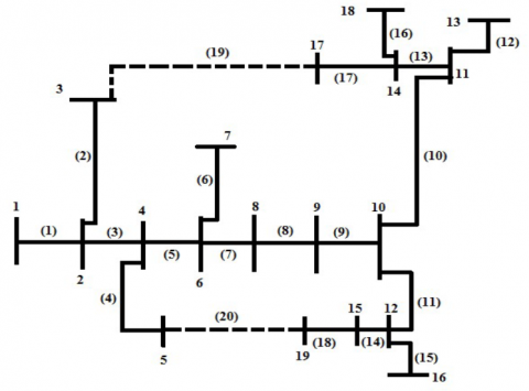
Figure 5 is a representation of the 19-node system that is described by Chen and Yang [23]. For the purpose of making the flow of power more manageable, the base voltage has been set to 11000V, and the base kVA has been set at 103 kVA. With a power supply optimization (PSO) of 11.497 kW and a projected CSA of 11.4012 kW, the actual power consumption without DG is 13.4709 kW. On the other hand, the wattles power consumption devoid of DG is 5.7956 kVAr, while the PSO level is 4.9464 kVAr and the projected CSA level is 4.9054 kVAr. We can examine how the voltage magnitude and phase angles of the 19-node URDN changed after the feeder was rewired by looking at Table 1. As a result of the addition of DG by CSA, the minimum voltages for the rewired network have increased to 0.9516 for phase a, 0.9498 for phase b, and 0.9505 for phase c. These values represent an increase from 0.9574, 0.9556, and 0.9559 p.u.
Table 1. Phase voltages of 19-node devoid of DG
|
Node |
Va |
angVa |
Vb |
angVb |
Vc |
angVc |
|
1 |
1.00000 |
0.00000 |
1.00000 |
-2.09450 |
1.00000 |
2.09450 |
|
2 |
0.98750 |
0.00030 |
0.98910 |
-2.09400 |
0.98800 |
2.09530 |
|
3 |
0.98540 |
0.00000 |
0.98870 |
-2.09410 |
0.98630 |
2.09580 |
|
4 |
0.98240 |
0.0006 0 |
0.98390 |
-2.09390 |
0.98300 |
2.09550 |
|
5 |
0.98200 |
0.0006 0 |
0.98370 |
-2.09390 |
0.9828 0 |
2.09560 |
|
6 |
0.97930 |
0.00070 |
0.98080 |
-2.09370 |
0.98010 |
2.09570 |
|
7 |
0.97860 |
0.00080 |
0.98030 |
-2.09380 |
0.97960 |
2.09570 |
|
8 |
0.97280 |
0.00110 |
0.97380 |
-2.09340 |
0.97350 |
2.09580 |
|
9 |
0.96590 |
0.00150 |
0.96600 |
-2.09290 |
0.96570 |
2.09590 |
|
10 |
0.95630 |
0.00190 |
0.95550 |
-2.09210 |
0.9550 |
2.09620 |
|
11 |
0.95500 |
0.00180 |
0.95430 |
-2.09190 |
0.95330 |
2.09630 |
|
12 |
0.9548 0 |
0.00200 |
0.9538 0 |
-2.09210 |
0.95360 |
2.09620 |
|
13 |
0.95440 |
0.00180 |
0.9534 0 |
-2.09170 |
0.9521 0 |
2.09630 |
|
14 |
0.95450 |
0.0018 0 |
0.95390 |
-2.09190 |
0.95280 |
2.09640 |
|
15 |
0.95270 |
0.00220 |
0.95120 |
-2.09190 |
0.95130 |
2.09620 |
|
16 |
0.95340 |
0.00230 |
0.9515 0 |
-2.09190 |
0.9522 0 |
2.09610 |
|
17 |
0.95370 |
0.00190 |
0.95340 |
-2.0920 0 |
0.95230 |
2.09650 |
|
18 |
0.9538 0 |
0.00180 |
0.9532 0 |
-2.0919 0 |
0.95210 |
2.096400 |
|
19 |
0.95160 |
0.00240 |
0.94980 |
-2.09190 |
0.95050 |
2.09620 |
Table 2. Phase voltages of 19-node with DG
|
Node |
Va |
angVa |
Vb |
angVb |
Vc |
angVc |
|
1 |
1.00000 |
0.0000 0 |
1.00000 |
-2.09440 |
1.00000 |
2.09440 |
|
2 |
0.98820 |
0.00050 |
0.98980 |
-2.09380 |
0.98870 |
2.09560 |
|
3 |
0.98610 |
0.00030 |
0.98940 |
-2.09380 |
0.98700 |
2.09610 |
|
4 |
0.98340 |
0.00100 |
0.98500 |
-2.09340 |
0.98410 |
2.09600 |
|
5 |
0.98310 |
0.00100 |
0.98470 |
-2.0935 0 |
0.98390 |
2.09600 |
|
6 |
0.98060 |
0.00130 |
0.98210 |
-2.09320 |
0.98140 |
2.09620 |
|
7 |
0.97990 |
0.0013 0 |
0.98160 |
-2.09330 |
0.98090 |
2.09620 |
|
8 |
0.97470 |
0.00190 |
0.97570 |
-2.09270 |
0.97540 |
2.09660 |
|
9 |
0.96850 |
0.00250 |
0.96860 |
-2.09180 |
0.96830 |
2.09700 |
|
10 |
0.96000 |
0.00340 |
0.95930 |
-2.09060 |
0.95880 |
2.097800 |
|
11 |
0.95870 |
0.00340 |
0.95810 |
-2.09040 |
0.95710 |
2.09790 |
|
12 |
0.95890 |
0.00370 |
0.95790 |
-2.09040 |
0.95770 |
2.09790 |
|
13 |
0.95820 |
0.00330 |
0.95720 |
-2.0902 0 |
0.95590 |
2.09790 |
|
14 |
0.95820 |
0.00340 |
0.95770 |
-2.09040 |
0.95660 |
2.09790 |
|
15 |
0.95800 |
0.00440 |
0.95650 |
-2.08970 |
0.95650 |
2.09840 |
|
16 |
0.9575 |
0.0040 |
0.95560 |
-2.09030 |
0.95630 |
2.09780 |
|
17 |
0.95740 |
0.00340 |
0.95710 |
-2.0905 0 |
0.95610 |
2.09800 |
|
18 |
0.95760 |
0.00340 |
0.95700 |
-2.09040 |
0.95590 |
2.09790 |
|
19 |
0.95770 |
0.00500 |
0.95590 |
-2.08930 |
0.95660 |
2.09880 |
Table 3. Outline of 19-node network
|
Parameters |
Devoid of DG |
with DG (PSO) |
with DG (CSA) |
||||||
|
a |
b |
c |
a |
b |
c |
a |
b |
c |
|
|
PTotal(kW) |
4.4539 |
4.4533 |
4.5637 |
3.8072 |
3.7964 |
3.8934 |
3.7783 |
3.7512 |
3.8717 |
|
QTotal(kVAr) |
1.9405 |
1.8964 |
1.9587 |
1.6587 |
1.6176 |
1.6701 |
1.6499 |
1.5986 |
1.6566 |
|
Vmini(p.u) |
0.9516 |
0.9498 |
0.9505 |
0.9553 |
0.9535 |
0.9542 |
0.9574 |
0.9556 |
0.9559 |
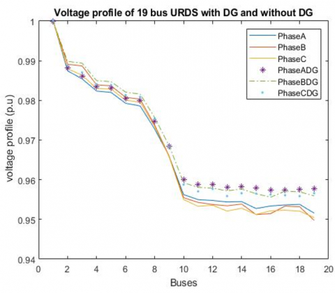
Table 2 examines the 19-node URDN voltage magnitude and phase angles, including DG. Figures 6 and 7 demonstrate the voltage change and power flow across all phases with and devoid of DG for 19 node URDN. DGs improve voltage profiles and reduce power losses. Table 3 summarizes CSA-based 19-node URDS with and without DG.
Figure 5. 19 bus URDS diagram
Figure 6. Voltage outline of 19-node devoid of DG
Figure 7. Voltage outline of 19-node network
4.2 25 – node with and devoid of DG
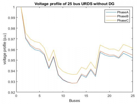
Figure 8 shows the 25-node system [23]. Base voltage is 4.16V and base kVA is 103 kva to improve power flow. Real electricity consumption without DG is 149.938 kW, with PSO 122.3192kW and projected CSA 107.1388kW. Devoid of DG, reactive power consumption is 166.9454 kVAr, with PSO 128.9192 and projected CSA 120.5875. The feeder rewiring affected the 25-bus unbalanced radial distribution system's voltage magnitude and phase angles, as shown in Table 4. The minimum voltages for the rewired network are 0.9284, 0.9285, and 0.9366 p.u., up from 0.9425, 0.9427, and 0.9483 with CSA adding DG.
Figure 8. 25-node URDS
Figure 9. Voltage outline of 25-node devoid of DG
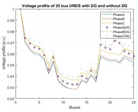
Figure 10. Voltage outline of 25-node network
Table 4. Phase voltages of 25-node devoid of DG
|
Node |
Va |
angVa |
Vb |
angVb |
Vc |
angVc |
|
1 |
1.00000 |
0.00000 |
1.00000 |
-2.0944 0 |
1.00000 |
2.09440 |
|
2 |
0.97020 |
-0.00990 |
0.97110 |
-2.10160 |
0.97550 |
2.08240 |
|
3 |
0.96320 |
-0.01220 |
0.96440 |
-2.10340 |
0.96980 |
2.07960 |
|
4 |
0.95980 |
-0.01340 |
0.96130 |
-2.10430 |
0.96740 |
2.07830 |
|
5 |
0.95870 |
-0.01330 |
0.96030 |
-2.1043 0 |
0.96640 |
2.07830 |
|
6 |
0.95500 |
-0.0097 0 |
0.95590 |
-2.10060 |
0.96150 |
2.08200 |
|
7 |
0.94190 |
-0.0097 0 |
0.94280 |
-2.0997 0 |
0.94920 |
2.08160 |
|
8 |
0.95290 |
-0.00970 |
0.95380 |
-2.10050 |
0.95960 |
2.08200 |
|
9 |
0.93590 |
-0.00970 |
0.93670 |
-2.09930 |
0.94380 |
2.08150 |
|
10 |
0.93150 |
-0.00970 |
0.93190 |
-2.09900 |
0.93950 |
2.08130 |
|
11 |
0.92940 |
-0.00970 |
0.92960 |
-2.09890 |
0.93760 |
2.08130 |
|
12 |
0.92840 |
-0.00970 |
0.92840 |
-2.09880 |
0.9366 0 |
2.08140 |
|
13 |
0.92870 |
-0.00970 |
0.92870 |
-2.09890 |
0.93680 |
2.08140 |
|
14 |
0.93590 |
-0.00960 |
0.93700 |
-2.09920 |
0.94340 |
2.08140 |
|
15 |
0.93380 |
-0.00960 |
0.93490 |
-2.09900 |
0.94140 |
2.08140 |
|
16 |
0.94080 |
-0.00970 |
0.94180 |
-2.09960 |
0.94830 |
2.08160 |
|
17 |
0.93470 |
-0.00960 |
0.93600 |
-2.09910 |
0.94200 |
2.08150 |
|
18 |
0.95730 |
-0.01220 |
0.95860 |
-2.10300 |
0.96430 |
2.07950 |
|
19 |
0.95480 |
-0.01220 |
0.95630 |
-2.10290 |
0.9620 |
2.07950 |
|
20 |
0.95350 |
-0.01220 |
0.95470 |
-2.10280 |
0.96030 |
2.07950 |
|
21 |
0.95380 |
-0.01210 |
0.95490 |
-2.10290 |
0.96050 |
2.07970 |
|
22 |
0.95180 |
-0.01210 |
0.95250 |
-2.10280 |
0.95850 |
2.07990 |
|
23 |
0.95650 |
-0.01330 |
0.95840 |
-2.10430 |
0.96480 |
2.07830 |
|
24 |
0.95440 |
-0.01330 |
0.95650 |
-2.10430 |
0.96310 |
2.07820 |
|
25 |
0.95200 |
-0.01320 |
0.95470 |
-2.10440 |
0.96120 |
2.07830 |
Table 5. Phase voltages of 19-node with DG
|
Node |
Va |
angVa |
Vb |
angVb |
Vc |
angVc |
|
1 |
1.00000 |
0.00000 |
1.00000 |
-2.09440 |
1.00000 |
2.09440 |
|
2 |
0.97420 |
-0.00460 |
0.97520 |
-2.09690 |
0.97820 |
2.08740 |
|
3 |
0.96730 |
-0.00690 |
0.96860 |
-2.09870 |
0.97260 |
2.08460 |
|
4 |
0.96380 |
-0.00800 |
0.96540 |
-2.09960 |
0.97020 |
2.08330 |
|
5 |
0.96280 |
-0.00800 |
0.96440 |
-2.09960 |
0.96920 |
2.08330 |
|
6 |
0.96390 |
-0.00090 |
0.96500 |
-2.09270 |
0.96850 |
2.09030 |
|
7 |
0.95580 |
0.00270 |
0.95690 |
-2.08850 |
0.96060 |
2.09330 |
|
8 |
0.96180 |
-0.00090 |
0.96290 |
-2.09260 |
0.96660 |
2.09020 |
|
9 |
0.94990 |
0.00270 |
0.95090 |
-2.08810 |
0.95520 |
2.09310 |
|
10 |
0.94560 |
0.00270 |
0.94610 |
-2.08780 |
0.95100 |
2.09300 |
|
11 |
0.94350 |
0.00270 |
0.94390 |
-2.08770 |
0.94910 |
2.09300 |
|
12 |
0.94250 |
0.00270 |
0.94270 |
-2.08770 |
0.94810 |
2.09300 |
|
13 |
0.94280 |
0.00270 |
0.94300 |
-2.08770 |
0.94830 |
2.09300 |
|
14 |
0.94990 |
0.00270 |
0.95120 |
-2.08800 |
0.95480 |
2.09310 |
|
15 |
0.94780 |
0.00280 |
0.94910 |
-2.08790 |
0.95290 |
2.09300 |
|
16 |
0.95950 |
0.00630 |
0.96070 |
-2.08510 |
0.96380 |
2.09670 |
|
17 |
0.94870 |
0.00280 |
0.95020 |
-2.08800 |
0.95350 |
2.09310 |
|
18 |
0.96140 |
-0.00690 |
0.96280 |
-2.09830 |
0.96710 |
2.08450 |
|
19 |
0.95890 |
-0.00690 |
0.96050 |
-2.09820 |
0.96480 |
2.08450 |
|
20 |
0.95760 |
-0.00690 |
0.95890 |
-2.09810 |
0.96310 |
2.08450 |
|
21 |
0.95790 |
-0.00680 |
0.95900 |
-2.09820 |
0.96340 |
2.08470 |
|
22 |
0.95590 |
-0.00670 |
0.95660 |
-2.09810 |
0.96130 |
2.08480 |
|
23 |
0.96050 |
-0.008000 |
0.96250 |
-2.09960 |
0.96760 |
2.08320 |
|
24 |
0.95850 |
-0.00800 |
0.96070 |
-2.09960 |
0.96590 |
2.08320 |
|
25 |
0.95610 |
-0.00790 |
0.95890 |
-2.09970 |
0.96400 |
2.08320 |
Table 6. Outline of 25-node network
|
Parameters |
Devoid of DG |
With DG (PSO) |
With DG (CSA) |
||||||
|
a |
b |
c |
a |
b |
c |
a |
b |
c |
|
|
PTotal (kW) |
52.7000 |
55.4102 |
41.8284 |
42.6411 |
44.9182 |
34.7599 |
37.5406 |
39.6744 |
29.9188 |
|
QTotal (kVAr) |
58.2048 |
53.0695 |
55.6711 |
44.6648 |
41.1201 |
43.1343 |
41.8358 |
38.4568 |
40.2949 |
|
V mini (p.u) |
0.9284 |
0.9285 |
0.9366 |
0.9325 |
0.9329 |
0.9394 |
0.9425 |
0.9427 |
0.9483 |
Table 7. CPU Time and iteration number of the suggested technique compared to method [15]
|
UBDN |
Without DG |
With DG |
||||||
|
CPU Time |
Iteration No. |
CPU Time |
Iteration No. |
|||||
|
CSA |
Method [15] |
CSA |
Method [15] |
CSA |
Method [15] |
CSA |
Method [15] |
|
|
19-node |
0.588632 |
3.130 |
3 |
6 |
0.116949 |
1.1312 |
3 |
6 |
|
25-node |
0.147372 |
2.180 |
5 |
7 |
0.179600 |
0.996 |
5 |
7 |
A discussion of the voltage magnitude and phase angles, including DG, of the unbalanced radial distribution system with 25 buses is shown in Table 5. Both Figure 9 and Figure 10 illustrate the magnitude and direction of the voltage change and power flow across all phases for a 25 node URDN, respectively, with and without the presence of Distributed Generation (DG). As a result of the incorporation of DG, the voltage profile is improved, and the real power losses are considerably reduced. In Table 6, a summary of 25-node URDS that either included or did not contain DG is presented using CSA. When compared to approach [15], the CPU Time and Iteration Number of the proposed CSA methodology are shown in Table 7.
An imbalanced radial distribution system's component modelling utilizing fundamental network theory principles has been provided, along with a power flow technique for solving it. The computing load is decreased by solving the voltage phasor's basic formulas. Unlike the time-consuming and inefficient forward-backward sweep approach, which requires repeated identification of parent-child buses, the algorithm only needs to identify the buses and branches beyond a single bus once. The algorithm's present way of summing has shown to provide reliable results. For practical R/X ratios, the suggested CSA approach has a strong convergence characteristic for the realistic URDS. As information is kept in vector form, a significant amount of computer memory is spared. When compared to the current technique presented by method, the CPU time required by the proposed CSA load-flow analysis for URDN is lower in all circumstances and the number of iterations is lower in certain cases.
Time spent evaluating objective functions, verifying established constraints through power-flow computing, and active losses all factor towards the total time spent calculating and determining the set of feasible solutions. In order for the suggested CSA method to work, power flow need not be optimum. An enhanced voltage outline feeder may avoid the need for the opening of sectionalizing switches. Because fewer switching operations are needed, less processing time is consumed in their place. Two test systems with asymmetric radial distributions are used to demonstrate the effectiveness of the suggested method. The suggested CSA technique is reducing real power losses from 13.4709 kW to 11.4012 kW and reactive power consumption from 5.7956 kvar to 4.9054 kvar and for 19-node URDS. Whereas for 25-node URDS reducing real power losses from 149.938 kW to 107.1388 kW and reactive power consumption from 166.9454 kvar to 120.5875 kvar.
[1] Kashem, M.A., Ganapathy, V., Jasmon, G.B. (1999). Network reconfiguration for load balancing in distribution networks. IEE Proceedings-Generation, Transmission and Distribution, 146(6): 563-567. https://doi.org/10.1049/ip-gtd:19990694
[2] Wagner, T.P., Chikhani, A.Y., Hackam, R. (1991). Feeder reconfiguration for loss reduction: An application of distribution automation. IEEE Transactions on Power Delivery, 6(4): 1922-1933. https://doi.org/10.1109/61.97741
[3] Vempalle, R., Dhal, P.K. (2020). Optimal placement of distributed generators in optimized reconfigure radial distribution network using PSO-DA optimization algorithm. In 2020 International Conference on Advances in Computing, Communication & Materials (ICACCM), Dehradun, India, pp. 239-246. https://doi.org/10.1109/ICACCM50413.2020.9213077
[4] Rafi, V., Dhal, P.K. (2020). Loss minimization based distributed generator placement at radial distributed system using hybrid optimization technique. In 2020 International Conference on Computer Communication and Informatics (ICCCI), Coimbatore, India, pp. 1-6. https://doi.org/10.1109/ICCCI48352.2020.9104145
[5] Jeon, Y.J., Kim, J.C. (2000). Network reconfiguration in radial distribution system using simulated annealing and tabu search. In 2000 IEEE Power Engineering Society Winter Meeting. Conference Proceedings (Cat. No. 00CH37077), Singapore, pp. 2329-2333. https://doi.org/10.1109/PESW.2000.847169
[6] Taylor, T., Lubkeman, D. (1990). Implementation of heuristic search strategies for distribution feeder reconfiguration. IEEE Transactions on Power Delivery, 5(1): 239-246. https://doi.org/10.1109/61.107279
[7] Askarzadeh, A. (2016). A novel metaheuristic method for solving constrained engineering optimization problems: Crow search algorithm. Computers & Structures, 169: 1-12. https://doi.org/10.1016/j.compstruc.2016.03.001
[8] Singh, D., Misra, R.K., Singh, D. (2007). Effect of load models in distributed generation planning. IEEE Transactions on Power Systems, 22(4): 2204-2212. https://doi.org/10.1109/TPWRS.2007.907582
[9] Marwali, M.N., Jung, J.W., Keyhani, A. (2007). Stability analysis of load sharing control for distributed generation systems. IEEE Transactions on Energy Conversion, 22(3): 737-745. https://doi.org/10.1109/TEC.2006.881397
[10] El-Samahy, I., El-Saadany, E. (2005). The effect of DG on power quality in a deregulated environment. In IEEE Power Engineering Society General Meeting, pp. 2969-2976. https://doi.org/10.1109/PES.2005.1489228
[11] Abou El-Ela, A.A., El-Sehiemy, R.A., Kinawy, A.M., Mouwafi, M.T. (2016). Optimal capacitor placement in distribution systems for power loss reduction and voltage profile improvement. IET Generation, Transmission & Distribution, 10(5): 1209-1221. https://doi.org/10.1049/iet-gtd.2015.0799
[12] Askarzadeh, A. (2016). Capacitor placement in distribution systems for power loss reduction and voltage improvement: A new methodology. IET Generation, Transmission & Distribution, 10(14): 3631-3638. https://doi.org/10.1049/iet-gtd.2016.0419
[13] Chou, H.M., Butler-Purry, K.L. (2014). Investigation of voltage stability in three-phase unbalanced distribution systems with DG using modal analysis technique. In 2014 North American Power Symposium (NAPS), pp. 1-6. https://doi.org/10.1109/NAPS.2014.6965388
[14] Ran, X., Miao, S. (2015). Probabilistic evaluation for static voltage stability for unbalanced three‐phase distribution system. IET Generation, Transmission & Distribution, 9(14): 2050-2059. https://doi.org/10.1049/iet-gtd.2014.1138
[15] Daratha, N., Das, B., Sharma, J. (2015). Robust voltage regulation in unbalanced radial distribution system under uncertainty of distributed generation and loads. International Journal of Electrical Power & Energy Systems, 73: 516-527. https://doi.org/10.1016/j.ijepes.2015.05.046.
[16] Calderaro, V., Galdi, V., Lamberti, F., Piccolo, A., Graditi, G. (2014). Voltage support control of unbalanced distribution systems by reactive power regulation. In IEEE PES Innovative Smart Grid Technologies, Europe, Istanbul, Turkey, pp. 1-5. https://doi.org/10.1109/ISGTEurope.2014.7028911
[17] Dahal, S., Salehfar, H. (2016). Impact of distributed generators in the power loss and voltage profile of three phase unbalanced distribution network. International Journal of Electrical Power & Energy Systems, 77: 256-262. https://doi.org/10.1016/j.ijepes.2015.11.038
[18] Ganguly, S., Sahoo, N.C., Das, D. (2013). Recent advances on power distribution system planning: A state-of-the-art survey. Energy Systems, 4: 165-193. https://doi.org/10.1007/s12667-012-0073-x
[19] Sathiskumar, M., Lakshminarasimman, L., Thiruvenkadam, S. (2012). A self adaptive hybrid differential evolution algorithm for phase balancing of unbalanced distribution system. International Journal of Electrical Power & Energy Systems, 42(1): 91-97. https://doi.org/10.1016/j.ijepes.2012.03.029
[20] Rafi, V., Dhal, P.K. (2020). Maximization savings in distribution networks with optimal location of type-I distributed generator along with reconfiguration using PSO-DA optimization techniques. Materials Today: Proceedings, 33: 4094-4100. https://doi.org/10.1016/j.matpr.2020.06.547
[21] Rafi, V., Dhal, P.K., Rajesh, M., Srinivasan, D.R., Chandrashekhar, M., Reddy, N.M. (2023). Optimal placement of time-varying distributed generators by using crow search and black widow-hybrid optimization. Measurement: Sensors, 30: 100900. https://doi.org/10.1016/j.measen.2023.100900.
[22] Vulasala, G., Sirigiri, S., Thiruveedula, R. (2009). Feeder reconfiguration for loss reduction in unbalanced distribution system using genetic algorithm. International Journal of Computer and Information Engineering, 3(4): 1050-1058.
[23] Chen, T.H., Yang, N.C. (2010). Loop frame of reference based three-phase power flow for unbalanced radial distribution systems. Electric Power Systems Research, 80(7): 799-806. https://doi.org/10.1016/j.epsr.2009.12.006
[24] Subrahmanyam, J.B.V. (2009). Load flow solution of unbalanced radial distribution systems. Journal of Theoretical and Applied Information Technology, 6(1): 040-051.
[25] Zimmerman, R.D., Chiang, H.D. (1995). Fast decoupled power flow for unbalanced radial distribution systems. IEEE Transactions on Power Systems, 10(4): 2045-2052. https://doi.org/10.1109/59.476074
[26] Ranjan, R., Venkatesh, B., Chaturvedi, A., Das, D. (2004). Power flow solution of three-phase unbalanced radial distribution network. Electric Power Components and Systems, 32(4): 421-433. https://doi.org/10.1080/15325000490217452.
[27] Hosseinzadeh, F., Alinejad, B., Pakfa, K. (2009). A new technique in distribution network reconfiguration for loss reduction and optimum operation. In CIRED 2009-20th International Conference and Exhibition on Electricity Distribution-Part 1, Prague, Czech Republic, pp. 1-3. https://doi.org/10.1049/cp.2009.0778
[28] Vempalle, R., Dhal, P.K. (2020). Loss minimization by reconfiguration along with distributed generator placement at radial distribution system with hybrid optimization techniques. Technology and Economics of Smart Grids and Sustainable Energy, 5: 1-12. https://doi.org/10.1007/s40866-020-00088-2