Abhishek Kumar*![]() | Om Prakash
| Om Prakash![]()
© 2024 The authors. This article is published by IIETA and is licensed under the CC BY 4.0 license (http://creativecommons.org/licenses/by/4.0/).
OPEN ACCESS
With the growing demand of low-cost transportation service, Hybrid airship plays a significant role for providing this service as a cargo nowadays. This paper deals with the controller design for winged hybrid airship with suspended payload for maintaining stability and controllability of the system. Controller design is required for the system to achieve desired tracking performance and collision avoidance for closed loop analysis. Internal Model Control (IMC) compensator is also designed to make few subsystems represented as velocity transfer function stable. The system is a small sized winged hybrid airship with attached suspended payload and having controlling maneuvers like elevator. The system taken is discussed as an approach of single body longitudinal dynamics. A Proportional-Integral-Derivative (PID) controller has been designed for pitch control of hybrid airship including collision avoidance in the pitch up and pith down path. A Hardware-In-the-Loop (HIL) solution also provided for the designed PID controller on UNO kit. Open loop and closed loop stability analysis is done for the longitudinal dynamics of winged small sized hybrid airship. Internal model compensator is required to make overall system as a stable system. A Simulink model for longitudinal dynamics of the hybrid airship with controllers and compensators is developed and result is analyzed and verified with open literature. Overshoot of u is the problem, although it settles to zero trim values within 30 sec. Except that all other parameters of longitudinal dynamics settle to equilibrium points within few seconds. Altair Embed software is used for HIL development.
hybrid airship, transportation, payload, longitudinal dynamics, controller design, Proportional-Integral-Derivative, Internal Model Control
The components of a traditional airship are a propulsion system, a gondola carrying payloads, a teardrop-shaped hull filled with lifting gas, and tail fins for stability and control. As lifting gases, helium and hydrogen are frequently utilized. Because they travel at a slow speed—roughly 20 m/s—airships are wind-sensitive. Throughout flight, the airship's weight and trim settings must be continuously adjusted to preserve stability. Due to its promising features, which include the capacity to hover, prolonged durability, low power consumption and heavy lifting, curiosity in hybrid airship design has been evolving. The characteristics of both heavier-than-air and lighter-than-air vehicles are combined in a hybrid airship. In addition to the propulsion system, buoyancy and aerodynamics also provide lift [1, 2].
Thanks to its static lift and the contribution of the wings to the stability and control of the aircraft, the hybrid-wing airship can be maintained for longer. The fuselage's integrated wings also allow the aircraft to descend safely, the aircraft can control the operation of the wing if there is a malfunction such as loss of helium in flight, and when the engine is not running the airship can glide while still having some tilt maneuverability control. If the hybrid wing airship is well designed, it can meet the requirements of a low-cost cargo vehicle with durability and good maneuverability, enabling it to move or travel in long space. The longitudinal dynamics of the mixed-wing lift airship are important to the safety and stability of the aircraft. Another important consideration in the design of the hybrid airship longitudinal dynamic controller is the control of the wings and elevators. Wings and elevators are important for controlling the pitch and speed of an airplane. Some researchers have suggested different management strategies to solve this problem.
Researchers have developed control strategies for hybrid airships to maintain pitch angle and speed while reducing wind gusts. Different control methods have been proposed, including feedback linearization [3], vision-based and station-keeping PID controllers [4]. The AURORA project focuses on developing detection, control, and navigation technologies for autonomous or semi-autonomous airships discussed by de Paiva et al. [5]. Another approach [6] uses a PID controller with gain developed using the H2/H∞ method. A dynamic inversion control law is also designed for path-tracking capability [7]. A hybrid aircraft payload system [8] is implemented with NDI using a 9 DOF nonlinear dynamic model. The design of two MIMO sliding mode controllers is presented by de Paiva et al. [9]. In relation to a particular reference trajectory, a trajectory tracking approach reduces angle and distance tracking errors. Kumar and Prakash [10] demonstrated how a predictive model of aircraft lateral dynamics is created using system detection. This article also discusses the creation of a state space model for a nonlinear problem. An autonomous airship's stabilisation and trajectory tracking issues are looked at in Zhang et al. [11]. The dynamics of the error systems are generated through the definition of new configuration and velocity errors. State feedback control rules are developed using the Lyapunov stability approach, and Matrosov's theorem is used to show that closed-loop fault systems are uniformly asymptotically stable. Repoulias and Papadopoulos [12] demonstrated a new closed-loop trajectory tracking controller that, using just three controllers, stabilises the position, orientation, linear, and angular velocity sets for a 3D flying robotic airship in a limited range near zero. Due to the sequential nature of vehicle dynamics, backstepping is employed. Additionally, it offers design adaptability and resistance to external shocks and parametric uncertainty. In Kulczycki et al. [13], the autonomous waypoint navigation of airships is examined using both a sequential loop closure controller (SLC) with classical inspiration and a hybrid classical/linear-quadratic regulator (LQR) controller. The LQR controller typically takes less time and fewer inputs in common navigation profiles and existing controller models. Atmeh and Subbarao [14] hypothesised that an AS500 aircraft can be flown through numerous waypoints in crosswind and time-varying wind circumstances by a straightforward LQ controller that receives navigation commands based on a relative navigation guidance law or a track-specific navigation guidance law. When just measurements from GPS and IMU sensors are available, a timed extended Kalman filter with a set of precomputed Jacobians performs reasonably well and offers reasonable estimates of states, measurement bias, and prevailing wind. It was discovered that using information about anticipated wind speeds can enhance the control instructions provided to the LQ controller, improving performance. When the airship couldn't land in Takaya et al. [15], a retry mode was added, and a loading landing function was developed. Wu [16] discussed a novel idea for an airship without thrust, rudder, or elevator. It is propelled by an interior air bubble with a variable mass and a moving mass. The input-output linearization, maximum feedback linearization, and internal stability of the LQR approach are used to analyse and control the dynamics of the longitudinal plane. Instead of the scaled configurations utilised in the wind tunnel test setup, a genuine geometric configuration is employed to simulate the results in Ashraf and Choudhry [17]. Using the bifurcation method, Kumar and Prakash [18] provided a 3DOF and 4DOF longitudinal hybrid airship model with longitudinal trim stability evaluation. For a variety of elevator deviation instances, trim analysis and simulation of a 3DOF hybrid airship model are conducted. The real flight controller for the hybrid airship with a suspended payload is designed using the collected results. Kumar and Prakash [19] developed a 3-DOF nonlinear longitudinal dynamic model for hybrid airships. For a hybrid airship with a suspended payload, a 4 DOF nonlinear longitudinal dynamic model is created. The simulation shows that the model almost behaves like a single-body 3 DOF longitudinal model. The fin deflection control motions that are unique to the hybrid model with three degrees of freedom (3DOF) are included, and in the four degree of freedom (4DOF), a new finding is the ability to regulate how the airship climbs by varying the angle of the rigging. However, this hybrid airship design is distinct. Its modelling and stability study were done in Ghaffar [20] using a process that is common for conventional aircraft and aeroplanes. The outcome demonstrates the winged hybrid airship's dynamic instability in lateral slow motion and longitudinal angular motion. This is a result of the close connection between the aerodynamic lift of the wing and the aerostatic lift of the buoyant gas. The findings of aerodynamic analyses on an early concept for a hybrid airship with wings are shown in Andan et al. [21]. Using a commercial CFD solvent and wind tunnel testing, the proposed model was effectively simulated. Data from wind tunnel tests and CFD simulation are compatible. Discuss the airship's equation of motion and the design of its tail fin in Cook [22]. Sinha and Ananthkrishnan [23] made contributions to the advancement of longitudinal dynamics control and airship dynamics. This book is an airship reference [24], and it discusses development of the linear longitudinal model for airships stability in heaviness condition. In Prakash [25], it is examined how the lateral inclination (rigging) of the hybrid airship suspension lines affects lateral and unidirectional flight dynamics.
In order to examine the flying behaviour of airships, such as in Cook et al. [26], and to build controls, as was done for a large airship [27], linear dynamic models have been employed extensively. An LTA vehicle's CG is below the CV, which causes the aircraft to have fluctuating pitch and roll angles. a motion resembling a pendulum. Analytical linear models [26, 28, 29] or numerical models created from finite difference nonlinear equations [30] have both been used to analyse airship stability. By analysing the eigenvalues and eigenvectors of the state matrices of the linear models, these stability investigations are carried out. According to the stability analysis results [26, 28-30], each mode of motion for conventional airships has identical motion characteristics. The surge subsidence damping mode, or a 1-DOF surge motion u, is the initial mode in the longitudinal plane and is brought on by the aerodynamic axial drag. The heave-pitch subsidence mode, which is brought on by typical aerodynamic drag, is the second longitudinal mode. As the velocity increases, the predominate motion is zero motion with near-zero velocity, some pitch angle y, and some pitch q. The airship's CG is located below the CV, which results in a pitch oscillatory mode, which is the origin of the third longitudinal pattern. Pitch rate q is the primary motion at almost zero velocity; as velocity rises, w becomes apparent.
Only two states can become unstable, according to the findings of the stability analysis [26, 28-30]. The characteristic values for the steady motion speeds u0 of 3,4,8 and 12m/s reveal that the Lotte airship's pitch incidence oscillation mode and sideslip yaw subsidance mode become unstable as the speed increases. This is so that the unstable Munk moment, which dominates the stabilizing moment generated by the fins [29], can be understood. Due to increased aerodynamic damping, all other modes stabilize as speed rises. The objective of the paper is to make the hybrid airship autonomous. In line with this approach a PID controller is designed for pitch control and for collision avoidance in pitch up and pitch down motion. For the same designed controller, HIL solution is also provided, and the controller is fabricated on UNO hardware kit interfaced with servo motor for hardware replica demonstration. Open loop and closed loop system stability analysis is also performed. IMC compensator is designed to make the system stable for velocity transfer functions. Longitudinal dynamic mode is also taken care.
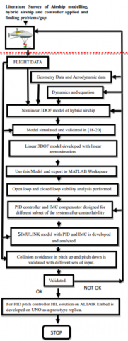
Figure 1. Methodology flow chart
Only two states can become unstable, according to the findings of the stability analysis [26, 28-30]. The characteristic values for the steady motion speeds u0 of 3,4,8 and 12m/s reveal that the Lotte airship's pitch incidence oscillation mode and sideslip yaw subsidance mode become unstable as the speed increases. This is so that the unstable Munk moment, which dominates the stabilizing moment generated by the fins [29], can be understood. Due to increased aerodynamic damping, all other modes stabilize as speed rises.
The objective of the paper is to make the hybrid airship autonomous. In line with this approach a PID controller is designed for pitch control and for collision avoidance in pitch up and pitch down motion. For the same designed controller, HIL solution is also provided, and the controller is fabricated on UNO hardware kit interfaced with servo motor for hardware replica demonstration. Open loop and closed loop system stability analysis is also performed. IMC compensator is designed to make the system stable for velocity transfer functions. Longitudinal dynamic mode is also taken care.
Methodology is shown in Figure 1.
The organisation of the paper is as follows: Section 1 starts with introduction to hybrid airship, it’s applications and literature survey of various control strategies adopted. Section 2 developed mathematical model for the hybrid airship in longitudinal dynamics in state space form and transfer function form primarily with elevator deflection as input for pitch control. Section 3 discuss about the open loop stability analysis of hybrid airship. Section 4 deals with closed loop stability analysis of hybrid airship including PID controller design for pitch control, IMC compensator design for making a system stable and HIL development on UNO hardware kit for pitch control with the help of servo motor as a hardware prototype replica for PID pitch controller. Result is simulated and analysed on SIMULINK. Collision avoidance is also taken care in this section. The work is concluded in section 5.
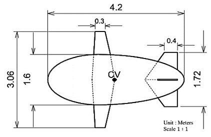
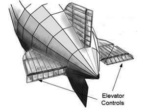
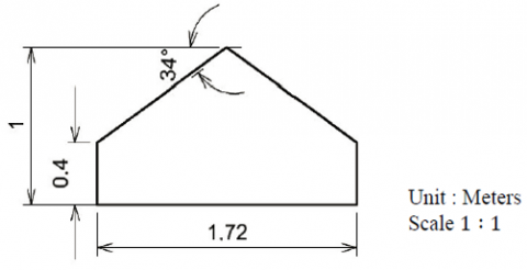
Mathematical modelling talks about the aerodynamics of airships and how factors like the interaction between the body and fins [31], separation between fins, and presence of fins affects lift. It mentions some studies that analyzed models like the R-101 and Akron and found fins separated by the hull produced around 30-40% more lift than directly connected fins. The drag on the hull is reported to be between 50-75% [31] while drag on tail fins is between 7-27% [1]. It also describes a hybrid airship model combining features of winged aircraft and airships, with a symmetric cross-shaped horizontal and vertical tail configuration at the rear end of the hull. The aerodynamic calculations consider forces from the hull as well. Figure 2 is a geometric top view of a hybrid winged airship. Figure 3 shows the control input as elevator deflection of horizontal tail of airship. Figure 4 is indicating the finite tail geometry used in the airship. It is common to define the hull reference area as $V^{\frac{2}{3}}$, and reference chord as $V^{\frac{1}{3}}$, where volume of the hull $V=\frac{2}{3} \pi\left(a_1+a_2\right) b^2$.
Figure 2. Top view of winged hybrid airship [20]
Figure 3. Elevator control on airship [1]
Figure 4. Finite tail geometry of airship [20]
Table 1. Airship geometry [20]
|
Parameter of a HULL |
Value |
|
Mass of a Hull, mh |
10 kg |
|
Overall Airship length, l |
3.75 m |
|
Maximum Airship Diameter, D |
1.6 m |
|
Hull Volume, V |
5.6 m3 |
|
Reference Area of a Hull, Sk |
3.16 m2 |
|
Reference length of a Hull, c |
1.78 m |
|
Ellipsoid shaped semi-minor axis, b |
0.8 m |
|
a1 |
1.55 m |
|
a2 |
2.75 m |
|
Airship Wingspan, bw |
3.06 m |
|
Airship Wing area, Sw |
1.72 m2 |
|
Airship tail span, bt |
3.06 m |
|
Airship tail area, St |
0.916 m2 |
|
Rck |
0.8 m |
|
Wing MAC $\bar{c}$ (m) |
0.47 |
|
Tail MAC $\bar{c}$ (m) |
0.51 |
Table 1 shows the geometry data used in modelling and simulation of the hybrid airship. For developing the mathematical model, it is assumed to be a flat earth approach, the aircraft is a rigid body, the mass and volume of the hybrid airship are constant, the volume averaged, and the average lift force assumed. coincident and air is assumed to be stationary. In addition to adding mass and inertia effects and lift, the equation of motion for the airship was developed using Newton's and Euler's equations. Longitudinal non-linear dynamic model of hybrid airship is developed by Kumar and Prakash [18, 19]. The linearization is done with small perturbation theory [22-24]. The linearized longitudinal dynamic equation [18] of the hybrid airship is as follows:
Force equations:
Axial force:
$\begin{aligned} & m_x \dot{U}+\left(m a_x-X_{\dot{q}}\right) \dot{q} \\ & \quad=X_1+X_u \cdot u+X_w \cdot w+X_{\delta_e} \cdot \delta_e \\ & \quad+\left(X q-m_z W_1\right) \cdot q \\ & \quad-(m g-B) \left(\sin \theta_1+\theta \cos \theta_1\right) \\ & \quad+T\end{aligned}$ (1)
Normal force:
$\begin{aligned} & m_z \dot{W}-\left(m a_x+Z_{\dot{q}}\right) \dot{q} \\ & \quad=Z_1+Z_u \cdot u+Z_w \cdot w+Z_{\delta_e} \cdot \delta_e \\ & \quad+\left(Z _q+m_x U_1\right) \cdot q \\ & \quad+(m g-B) \left(\cos \theta_1-\theta \sin \theta_1\right)\end{aligned}$ (2)
Moment equations:
Pitching moment:
$\begin{gathered}J_y \dot{q}+\left(m a_z+M_{\dot{u}}\right) \dot{U}-\left(m a_x+M_{\dot{w}}\right) \dot{W} \\ =M_1+M_u \cdot u+M_w \cdot w+M_{\delta_e} \cdot \delta_e \\ \left.+(M)_q-m a_x U_1-m a_z W_1\right) \cdot q \\ -\theta\left[\left(m g a_z+B b_z\right) \cos \theta_1\right. \\ -\left(m g a_x+B b_x\right) \sin \left[\theta_1\right] \\ -\left(m g a_z+B b_z\right) \sin \theta_1 \\ -\left(m g a_x+B b_x\right) \cos \theta_1+T d_z\end{gathered}$ (3)
Kinematic equation:
$\dot{\theta}=q$ (4)
2.1 State space representation of linearized longitudinal dynamic equations for hybrid airship
Eqs. (1) to (4) are expressed in state space form as:
$m \dot{x}=a x+b u$ (5)
where, the state variables expressed as:
$x^T=\left[\begin{array}{llll}u & w & q & \theta\end{array}\right]$ (6)
$u^T=\left[\delta_e T\right]$ (7)
The state variable in Eq. (6), u is forward velocity along x body axis of airship, w is the velocity in z body axis of airship, q is pitching moment along y body axis of airship and θ is the pitching angle. Eq. (7) is the input variable vectors having δe as elevator deflection and T is thrust, where,
$m=\left[\begin{array}{cccc}m_x & 0 & \left(m a_x-X_{\dot{q}}\right) & 0 \\ 0 & m_z & -\left(m a_x+Z_{\dot{q}}\right) & 0 \\ \left(m a_z+M_{\dot{u}}\right) & -\left(m a_x+M_{\dot{w}}\right) & J_y & 0 \\ 0 & 0 & 0 & 1\end{array}\right]$
$a=$$\left[\begin{array}{cccc}X_u & X_w & \left(X_q-m_z W_1\right) & -(m g-B) \cos \theta_1 \\ Z_u & Z_w & \left(Z_q+m_x U_1\right) & -(m g-B) \sin \theta_1 \\ M_u & M_w & \left(M_q-m a_x U_1-m a_z W_1\right) & -\left[\left(m g a_z+B b_z\right) \cos \theta_1-\left(m g a_x+B b_x\right) \sin \theta_1\right] \\ 0 & 0 & 1 & 0\end{array}\right]$
$b=\left[\begin{array}{cc}{\left[X_{\delta_e}+C_{L_{\delta_e}} \sin \alpha-C_{D_{\delta_e}} \cos \alpha\right]} & 1 \\ {\left[Z_{\delta_e}-C_{D_{\delta_e}} \sin \alpha-C_{L_{\delta_e}} \cos \alpha\right]} & 0 \\ {\left[M_{\delta_e}+C_{m_{\delta_e}}\right]} & d_z \\ 0 & 0\end{array}\right]$
The general form of the state equation represented in Eq. (8) as:
$\dot{x}=A x+B u$ (8)
where, system matrix A=m-1a, Input matrix B= m-1b.
2.2 Aerodynamic model of longitudinal dynamic equations for hybrid airship
The equation for aerodynamic forces and moments are provided below [1, 25]. Let δELVL and δELVR be the deflections of the left and right trailing edge flaps of the elevator.
$\begin{aligned} X=\frac{1}{2} \rho V_0^2 & {\left[C_{X_1} \cos ^2 \alpha \cos ^2 \beta\right.} \\ & \left.+C_{X_2} \sin 2 \alpha \sin \left(\frac{\alpha}{2}\right)\right] \end{aligned}$ (9)
$\begin{gathered}Z=\frac{1}{2} \rho V_0^2\left[C_{Z_1} \cos \left(\frac{\alpha}{2}\right) \sin 2 \alpha+C_{Z_2} \sin (2 \alpha)\right. \\ +C_{Z_3} \sin (\alpha) \sin (|\alpha|) \\ \left.+C_{Z_4}\left(\delta_{E L V L}+\delta_{E L V R}\right)\right]\end{gathered}$ (10)
$\begin{gathered}M=\frac{1}{2} \rho V_0^2\left[C_{M_1} \cos \left(\frac{\alpha}{2}\right) \sin 2 \alpha+C_{M_2} \sin (2 \alpha)\right. \\ +C_{M_3} \sin (\alpha) \sin (|\alpha|) \\ \left.+C_{M_4}\left(\delta_{E L V L}+\delta_{E L V R}\right)\right]\end{gathered}$ (11)
$C_L=\left\{C_{L_0}+C_{L_\alpha} \cdot \alpha+C_{L_q} \cdot \frac{q \bar{c}}{2 V_1}+C_{L_{\delta_e}} \cdot \delta_e\right\}$ (12)
$C_D=\left\{C_{D_0}+C_{D_\alpha} \cdot \alpha+C_{D_q} \cdot \frac{q \bar{c}}{2 V_1}+C_{D_{\delta_e}} \cdot \delta_e\right\}$ (13)
$C_m=\left\{C_{m_0}+C_{m_\alpha} \cdot \alpha+C_{m_q} \cdot \frac{q \bar{c}}{2 V_1}+C_{m_{\delta_e}} \cdot \delta_e\right\}$ (14)
The expression for the stability derivatives is given in the Table 2. The aerodynamic coefficients (such as, $C_{m_\alpha}, C_{m_q}$ and $c_{m_{\delta_e}}$) are obtained as shown in Table 3, either from wind tunnel test, numerical solutions, or semi-empirical approach [21].
Table 2. Longitudinal stability derivatives [1, 21]
|
u Derivatives |
w Derivatives |
|
$\begin{aligned} X_u & =\frac{-2 C_{D_1} q_1 S}{U_1} \\ Z_u & =\frac{-2 C_{L_1} q_1 S}{U_1} \\ M_u & =\frac{C_{m_1} q_1 S \bar{c}}{U_1}\end{aligned}$ |
$\begin{gathered}X_w=\frac{-\left(C_{D_\alpha}-C_{L_1}\right) q_1 S}{U_1} \\ Z_w=\frac{-\left(C_{L_\alpha}+C_{D_1}\right) q_1 S}{U_1} \\ M_w=\frac{C_{m_\alpha} q_1 S \bar{c}}{U_1}\end{gathered}$ |
|
q Derivatives |
δe Derivatives |
|
$\begin{aligned} X_q & =\frac{-C_{D_q} q_1 S \bar{c}}{2 U_1} \\ Z_q & =\frac{-C_{L_q} q_1 S \bar{c}}{2 U_1} \\ M_q & =\frac{C_{m_q} q_1 S \bar{c}^2}{2 U_1}\end{aligned}$ |
$\begin{aligned} X_{\delta_e} & =\frac{-C_{D_{\delta_e}} q_1 S \bar{c}}{2 U_1} \\ Z_{\delta_e} & =\frac{-C_{L_{\delta_e}} q_1 S \bar{c}}{2 U_1} \\ M_{\delta_e} & =\frac{C_{m_{\delta_e}} q_1 S \bar{c}^2}{2 U_1}\end{aligned}$ |
Table 3. Aerodynamic coefficient data [17, 20, 21, 32]
|
Aerodynamic Coefficient |
Approximate Equations |
Estimated Values for Hybrid Airship |
|
$C_{D_\alpha}$ |
$2 C_{L_1} C_{L_\alpha} K$, where $\mathrm{K}=\frac{1}{\pi e A R}$ is induced drag factor. |
0.0011 |
|
$C_{L_\alpha}$ |
CFD |
0.0462 |
|
$C_{m_\alpha}$ |
CFD |
-0.0066 |
|
$C_{D_q}$ |
$-2 \eta_{h t} C_{D_{\alpha h t}} V_{h t}$ |
negligible |
|
$C_{L_q}$ |
$\begin{gathered}-2 \eta_{h t} C_{L_\alpha} V_{h t} \text {, where } \\ V_{h t}=\frac{l_h}{\bar{c}} \frac{S_{h t}}{S}, \eta_{h t}=1\end{gathered}$ |
-0.0104 $C_{L_{\alpha h t}}=0.0048$ -ve for canard configuration |
|
$C_{m_q}$ |
$-2 \eta_{h t} C_{L_\alpha h t} V_{h t} \frac{l_{h t}}{\bar{c}}$ |
-0.0359 |
|
$C_{D_{\delta_e}}$ |
$-\eta_{h t} C_{D_{\alpha h t}} V_{h t} \zeta \frac{S_{h t}}{S}$ |
$C_{D_{\alpha h t}}$ not available. 0.120 |
|
$C_{L_{\delta_e}}$ |
$-\eta_{h t} C_{L_{\alpha h t}} V_{h t} \zeta \frac{S_{h t}}{S}$
|
1.24 |
|
$C_{m_{\delta e}}$ |
$\begin{gathered}-\eta_{h t} C_{L_\alpha h t} V_{h t} \zeta, \text { where } \\ \zeta=0.62\end{gathered}$ |
-6.8 |
With the help of semi-empirical method, the mathematical model is developed on MATLAB and the state matrix A and the input matrix B is computed for the winged hybrid airship is computed for longitudinal dynamics as below:
$\begin{gathered}A=\left[\begin{array}{cccc}-0.3339 & 0.3763 & 0.0633 & -4.8697 \\ -1.2535 & -0.5901 & 34.1954 & 0 \\ -0.1094 & 0.0809 & -0.0286 & 1.1979 \\ 0 & 0 & 1 & 0\end{array}\right] \\ B=\left[\begin{array}{cc}-0.0032 & 0.1113 \\ 0.0056 & 0 \\ -0.0022 & 0.0027 \\ 0 & 0\end{array}\right]\end{gathered}$
To design a controller for a system represented in state space form, the Kalman controllability test is checked. If the system matrix A is of order n×n, Then, we create the controllability matrix (Qc):
$\mathrm{Qc}=\left[B: A B: A^2 B: A^3 B\right]$
The calculated value of Qc for the system is:
$\begin{aligned} & \text { Qc }= {\left[\begin{array}{cccccccc}-0.0032 & 0.1113 & 0.0030 & -0.0370 & -0.0183 & -0.0193 & 0.0276 & -0.0634 \\ 0.0056 & 0 & -0.0745 & -0.0472 & 0.0698 & -0.3448 & -0.3267 & 0.3581 \\ -0.0022 & 0.0027 & 0.0009 & -0.0123 & -0.0090 & 0.0038 & 0.0089 & 0.3581 \\ 0 & 0 & -0.0022 & 0.0027 & 0.0009 & -0.0123 & -0.0090 & 0.0038\end{array}\right]}\end{aligned}$
Table 4. Hybrid airship system transfer function and designed controller transfer function for longitudinal dynamics
|
$\frac{O / p}{i / p}$ |
Transfer Function (O/p vs δe) |
|
$\mathrm{G} 11=\frac{u(s)}{\boldsymbol{\delta}_{\boldsymbol{e}}}$ |
$\frac{-0.0032(s-0.6215)\left(s^{\wedge} 2+0.6252 s+1.938\right)}{(s+2.294)(s-1.695)\left(s^{\wedge} 2+0.3534 s+0.4139\right)}$ |
|
$\mathrm{G} 12=\frac{w(s)}{\boldsymbol{\delta}_{\boldsymbol{e}}}$ |
$\frac{0.0056(s-12.66)\left(s^{\wedge} 2+0.3009 s+0.331\right)}{(s+2.294)(s-1.695)\left(s^{\wedge} 2+0.3534 s+0.4139\right)}$ |
|
$\mathrm{G} 13=\frac{q(s)}{\boldsymbol{\delta}_{\boldsymbol{e}}}$ |
$\frac{-0.0022 s\left(s^{\wedge} 2+0.5589 s+0.4634\right)}{(s+2.294)(s-1.695)\left(s^{\wedge} 2+0.3534 s+0.4139\right)}$ |
|
$\mathrm{G} 14=\frac{\theta(s)}{\boldsymbol{\delta}_{\boldsymbol{e}}}$ |
$\frac{-0.0022\left(s^{\wedge} 2+0.5589 s+0.4634\right)}{(s+2.294)(s-1.695)\left(s^{\wedge} 2+0.3534 s+0.4139\right)}$ |
|
$\frac{O / p}{i / p}$ |
Transfer Function (O/p vs $T$) |
|
$\mathrm{G} 21=\frac{u(s)}{T}$ |
$\frac{0.1113(s+2.179)(s-1.761)(s+0.2024)}{(s+2.294)(s-1.695)\left(s^{\wedge} 2+0.3534 s+0.4139\right)}$ |
|
$\mathrm{G} 22=\frac{w(s)}{T}$ |
$\frac{-0.047187(s+8.707)(s-0.4469)}{(s+2.294)(s-1.695)\left(s^{\wedge} 2+0.3534 s+0.4139\right)}$ |
|
$\mathrm{G} 23=\frac{q(s)}{T}$ |
$\frac{0.0027 s(s-4.857)(s+1.271)}{(s+2.294)(s-1.695)\left(s^{\wedge} 2+0.3534 s+0.4139\right)}$ |
|
$\mathrm{G} 24=\frac{\theta(s)}{T}$ |
$\frac{0.0027(s-4.857)(s+1.271)}{(s+2.294)(s-1.695)\left(s^{\wedge} 2+0.3534 s+0.4139\right)}$ |
The rank of Qc (controllability matrix) is 4 i.e., equal to the rank of system matrix A, so the system is controllable in the nature. Open loop Transfer function is obtained on MATLAB platform from the state space longitudinal model of the hybrid airship system with the help of Laplace transform technique and shown in the Table 3. The Controller transfer function is also mentioned in the Table 4.
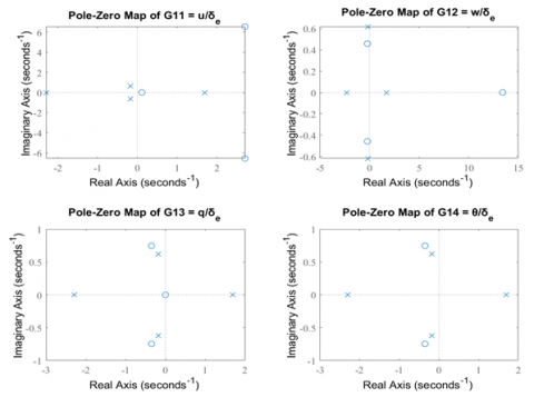
Eigenvalues of the hybrid airship system is obtained from its characteristic equation |SI-A|=0 or the denominator of any transfer function equal to zero. Where I is 4×4 identity matrix. The obtained eigen values for the hybrid airship are two real -2.2940 and 1.6948 and one complex pair of roots -0.1767+0.6186i and -0.1767-0.6186i. In summary, the hybrid airship’s longitudinal motion characteristic roots consist of a stable first order root, an unstable first order root and a pair of stable oscillatory roots. Our study is based on elevator deflection as an input in designing a controller /compensator for longitudinal dynamics of the system. The pole zero map for the systems is shown in Figure 5.
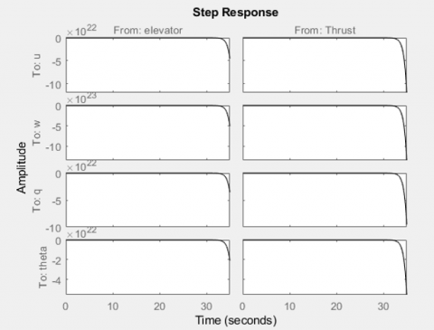
Open loop step response of the MIMO state space model (A, B, C, D) is shown in Figure 6 by observing the step response and pole zero map of the system, it is observed that the system is unstable in nature because one pole lies on RHS plane of pole zero map.
Figure 5. Pole zero map
Figure 6. Step response open loop
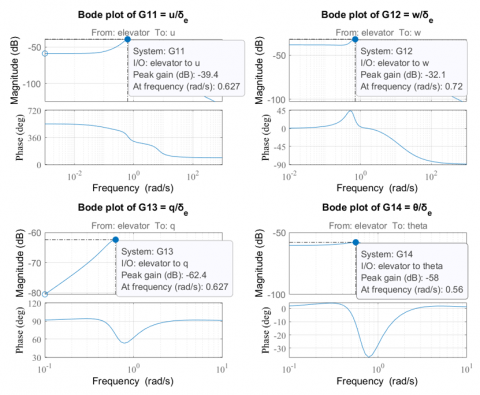
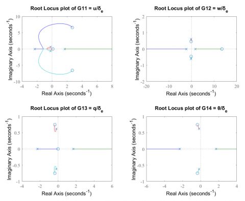
For closed loop stability analysis [14-16], root locus and bode plot technique is performed for each four-transfer function (O/p vs δe) discussed in Table 3. Bode plot and root locus for the system is shown in Figures 7 and 8 respectively.
Figure 7. Bode plot of the system
Figure 8. Root locus plot of the system
The small sized winged hybrid airship having elevator control maneuver surface and with suspended payload mathematical model is analysed in longitudinal dynamics. The mode analysis, damping factor, frequency, and time constant are calculated for each eigen values of the system and is listed in Table 5.
It is observed that the system in closed loop is not dynamically stable, so to make a system stable and having trajectory tacking mechanism, designing of controllers/compensators with filter is required. Pitch control is an important aspect in longitudinal dynamics of hybrid airship discussed in references [8-12]. For pitch control as a trajectory tracking, a PI and PID controller is designed for the transfer function $G 13=\frac{q(s)}{\delta_e} \quad$ and $\quad G 14=\frac{\theta(s)}{\delta_e}$. IMC compensator is designed for stabilizing the transfer function $G 11=\frac{u(s)}{\delta_e} \quad$ and $\quad G 12=\frac{w(s)}{\delta_e}$. The designed controller/compensator transfer function is listed in Table 6.
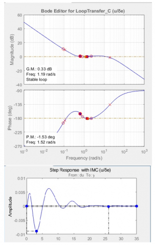
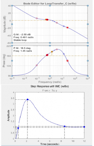
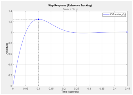
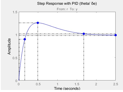
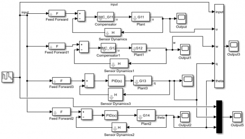
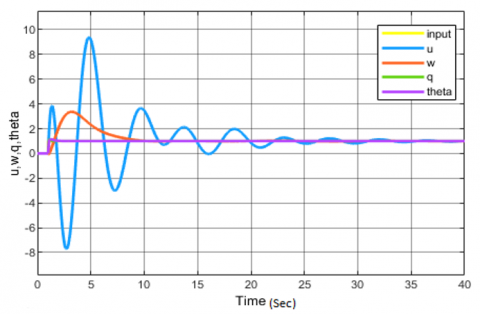
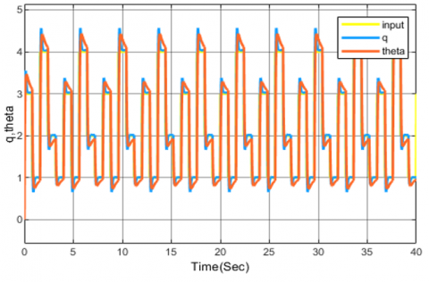
The performance, robustness, and stability analysis for transfer functions $\left(\frac{u(s)}{\delta_{\boldsymbol{e}}}, \frac{w(s)}{\delta_{\boldsymbol{e}}}, \frac{q(s)}{\delta_{\boldsymbol{e}}}\right.$ and $\left.\frac{\theta(s)}{\delta_{\boldsymbol{e}}}\right)$ are obtained and listed in Table 7. The same analysis is also done for the system with different controllers as required and is listed in Table 7. Eigen values of w, the velocity in z body axis of winged hybrid airship is on RHS of pole zero plot, that provides instability in the system. The winged hybrid airship is statically stable and dynamically unstable. An internal model control (IMC) compensator [13] is designed for a SISO mathematical model represented in transfer function form as G11 and G12. The bode plot and step response of IMC compensator for G11 and G12 are shown in Figure 9 and Figure 10 respectively and it gives closed loop stability in the system. PI (proportional integral) controller and PID (proportional integral derivative controller is designed as pitch control and trajectory tracking for G13 and G14 transfer function. The reference tracking response of G13 and G14 is shown in Figure 11 and Figure 12. Finally, a complete longitudinal dynamics model with controller/compensator for winged hybrid airship is designed as Simulink model and is shown in Figure 13. Simulink step response and collision avoidance pitch control response is shown in Figure 14 and Figure 15. respectively. u and w with compensator overshoots at higher value, so Hardware in loop (HIL) solution for the same is not possible here in this case due to the actuator movement limit.
Table 5. Longitudinal dynamics mode analysis
|
Transfer Function |
Pole/Longitudinal Eigen Values |
Damping |
Frequency (rad/s) |
Time Constant(s) |
Stability |
Mode |
|
$\begin{aligned} \mathrm{G} 11 & =\frac{u(s)}{\boldsymbol{\delta}_{\boldsymbol{e}}} \\ \mathrm{G} 12 & =\frac{w(s)}{\boldsymbol{\delta}_{\boldsymbol{e}}} \\ \mathrm{G} 13 & =\frac{q(s)}{\boldsymbol{\delta}_{\boldsymbol{e}}} \\ \mathrm{G} 14 & =\frac{\theta(s)}{\boldsymbol{\delta}_{\boldsymbol{e}}}\end{aligned}$ System matrix A |
-0.177 + 0.6191i |
0.275 |
0.643 |
5.66 |
yes |
Pendulum mode |
|
-0.177 - 0.6191i |
0.275 |
0.643 |
5.66 |
yes |
Pendulum mode |
|
|
1.69 |
-1 |
1.69 |
-0.59 |
no |
Heave mode |
|
|
-2.29 |
1 |
2.29 |
0.436 |
yes |
Surge mode |
Table 6. Controller transfer function for longitudinal dynamics of hybrid airship
|
|
Controller Transfer Function (O/p vs δe) |
|
G11_IMC |
$\frac{-7241.2(s+2.272)(s-0.8257)(s+0.09128)\left(s^2+0.397 s+0.4041\right)}{s(s-19.3)(s-0.1089)\left(s^2+0.6198 s+1.948\right)}$ |
|
G12_IMC |
$\frac{-597.06(s+23.98)(s+3.534)(s+0.09103)\left(s^{\wedge} 2+0.3099 s+0.4018\right)}{s\left(s^{\wedge} 2+0.2686 s+0.3322\right)\left(s^{\wedge} 2+47.47 s+646.9\right)}$ |
|
G13_PI |
$-13530.16\left(1+\frac{12.7037}{s}\right)$ |
|
G14_PID |
$-38070.787-\frac{39504.896}{s}-8952.545 \frac{109.82}{1+109.82 s}$ |
Table 7. Performance, robustness, and stability analysis
|
Transfer Function |
GM (dB) |
PM (dB) |
Rise Time |
Settling Time |
Overshoot |
Peak |
CL Stability |
|
$\mathrm{G} 11=\frac{u(s)}{\delta_e}$ |
52.4 dB @ 0 rad/s |
- |
- |
- |
- |
- |
NO |
|
$\mathrm{G} 12=\frac{w(s)}{\delta_e}$ |
- |
- |
- |
- |
- |
- |
NO |
|
$\mathrm{G} 13=\frac{q(s)}{\delta_e}$ |
- |
- |
- |
- |
- |
- |
NO |
|
$\mathrm{G} 14=\frac{\theta(s)}{\delta_e}$ |
- |
- |
- |
- |
- |
- |
NO |
|
G11_IMC |
0.33 dB @ 1.19 rad/s |
-1.53deg @1.52 rad/s |
0.0376 s |
28.9 s |
838.4% |
9.38 in 3.83 s |
YES |
|
G12_IMC |
-2.55 dB @ 0.491 rad/s |
18.5 deg @ 1.45 rad/s |
0.339 s |
8.59 s |
236% |
3.36 in 2.14 s |
YES |
|
G13_PI |
-37.8 @1.15 rad/s |
69 deg @ 31.9 rad/s |
0.0433 s |
0.264 s |
17.8% |
1.19 |
YES |
|
G14_PID |
-20.6 dB @ 2.02 rad/s |
69 deg @ 20.1 rad/s |
0.064 s |
1 s |
15.7 % |
1.16 |
YES |
Figure 9. G11_IMC compensator with system response
Figure 10. G12_IMC compensator with system response
Figure 11. G13_PI controller reference tracking
Figure 12. G14_PID controller reference tracking
Figure 13. Simulink longitudinal dynamic model for winged hybrid airship
Figure 14. Step response of Simulink model
Figure 15. Collision avoidance response
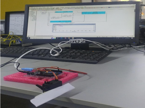
Figure 16. HIL for G14 as pitch control
Figure 17. Development of airship in UPES campus
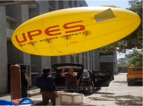
PID controller for pitch control is fabricated on UNO board with ALTAIR Embed software shown in Figure 16. The movement of elevator for pitch control is represented here with paper attached to servo motor. This is a small step to make hybrid airship autonomous with navigation, guidance, and control. The airship shown in Figure 17, is under development as a SEED funded project under Dr. Om Prakash in UPES, Dehradun campus. Result of longitudinal stability analysis of the hybrid airship is elaborated in Tables 5 and 7.
In this paper, a complete linearized mathematical model for longitudinal dynamics of winged hybrid airship with elevator deflection is developed in state space form and with transfer function classical approach. The work is in continuation with development and analysis of non-linear mathematical model of small sized winged hybrid airship with suspended payload discussed [18-20]. For longitudinal trim, the hybrid airship is flying at 20 m/s speed, pitch angle 0 degree and angle of attack as 0 degree. u, w, q and θ are states of the system and δe (elevator) and T (thrust) are inputs to the system. The work is restricted to elevator deflection as longitudinal dynamic study in this paper. The stability analysis is done for both open loop and closed loop. The winged hybrid airship is statically stable and dynamically unstable in nature. The time domain analysis and frequency domain analysis are done for the system. Aerodynamic model is developed with the help of curve tracing techniques on the graph taken from the study [21]. Aerodynamic data is computed either from wind tunnel test, numerical solutions, or semi-empirical approach approximating the dynamics is more towards conventional aircraft.
PID controller is tuned and designed for pitch control. IMC compensator is designed for u and w. After designing the controller, the system is stable in closed loop and pitch up and down trajectory tracking is achieved more accurately for hybrid airship. Hardware in loop solution is also provided in this paper as shown in Figure 16. With reference to the table 7, the hybrid airship system is unstable in open loop but is stable with proper designing of controllers and compensators. For G13 transfer function PI controller is designed for pitch control, and it settles within 0.264 s with rise time of 0.0433 s and overshoot of 17.8 percentage. For G14 transfer function PID controller is designed for pitch control, and it settles within 1 s with rise time of 0.064 s and overshoot of 15.7 percentage. In pitching path simulation of collision avoidance is shown in Figure 15.
The same work with controller design in this paper can be carried out for making the airship shown in Figure 15 as autonomous with geometrical values inserted. The airship shown in Figure 17 will be used for delivering a payload in small range transportation.
[1] Khoury, G.A. (2012). Airship Technology. Cambridge University Press.
[2] Ardema, M.D. (1977). Feasibility of modern airships: Preliminary assessment. Journal of Aircraft, 14(11): 1140-1148. https://doi.org/10.2514/3.58902
[3] Nagabhushan, B.L., Tomlinson, N.P. (1982). Dynamics and control of a heavy lift airship hovering in a turbulent cross wind. Journal of Aircraft, 19(10): 826-830. https://doi.org/10.2514/3.61564
[4] van der Zwaan, S., Bernardino, A., Santos-Victor, J. (2000). Vision based station keeping and docking for an aerial blimp. In Proceedings. 2000 IEEE/RSJ International Conference on Intelligent Robots and Systems (IROS 2000) (Cat. No. 00CH37113), Takamatsu, Japan, pp. 614-619. https://doi.org/10.1109/IROS.2000.894672
[5] de Paiva, E.C., Bueno, S.S., Gomes, S.B., Ramos, J.J., Bergerman, M. (1999). A control system development environment for AURORA's semi-autonomous robotic airship. In Proceedings 1999 IEEE International Conference on Robotics and Automation (Cat. No. 99CH36288C), Detroit, MI, USA, pp. 2328-2335. https://doi.org/10.1109/ROBOT.1999.770453
[6] Carvalho, J., De Paiva, E., Elfes, A., Azinheira, J., Ferreira, P., Ramos, J. (2001). Classic and robust PID heading control of an unmanned robotic airship. In SIRS 2001: Proceedings of the 9th International Symposium on Intelligent Robotic Systems, Toulouse, pp. 61-70.
[7] Moutinho, A., Azinheira, J.R. (2004). Path control of an autonomous airship using dynamic inversion. IFAC Proceedings Volumes, 37(8): 633-638. https://doi.org/10.1016/S1474-6670(17)32049-9
[8] Prakash, O., Kumar, A. (2022). NDI based heading tracking of hybrid-airship for payload delivery. In AIAA SCITECH 2022 Forum, p. 1432. https://doi.org/10.2514/6.2022-1432
[9] de Paiva, E.C., Benjovengo, F., Bueno, S.S. (2007). Sliding mode control for the path following of an unmanned airship. IFAC Proceedings Volumes, 40(15): 221-226. https://doi.org/10.3182/20070903-3-FR-2921.00040
[10] Kumar, A., Prakash, O. (2022). Analysis of lateral dynamics of ARX model of an aircraft with model predictive controller. In 2022 International Conference for Advancement in Technology (ICONAT), Goa, India, pp. 1-6. https://doi.org/10.1109/ICONAT53423.2022.9726117
[11] Zhang, Y., Qu, W.D., Xi, Y.G., Cai, Z.L. (2008). Stabilization and trajectory tracking of autonomous airship's planar motion. Journal of Systems Engineering and Electronics, 19(5): 974-981. https://doi.org/10.1016/S1004-4132(08)60184-X
[12] Repoulias, F., Papadopoulos, E. (2008). Robotic airship trajectory tracking control using a backstepping methodology. In 2008 IEEE International Conference on Robotics and Automation, Pasadena, CA, USA, pp. 188-193. https://doi.org/10.1109/ROBOT.2008.4543207
[13] Kulczycki, E., Joshi, S., Hess, R., Elfes, A. (2006). Towards controller design for autonomous airships using SLC and LQR methods. In AIAA Guidance, Navigation, and Control Conference and Exhibit, p. 6778. https://doi.org/10.2514/6.2006-6778
[14] Atmeh, G., Subbarao, K. (2016). Guidance, navigation and control of unmanned airships under time-varying wind for extended surveillance. Aerospace, 3(1): 8. https://doi.org/10.3390/aerospace3010008
[15] Takaya, T., Kawamura, H., Minagawa, Y., Yamamoto, M., Ohuchi, A. (2006). PID landing orbit motion controller for an indoor blimp robot. Artificial Life and Robotics, 10: 177-184. https://doi.org/10.1007/s10015-006-0385-9
[16] Wu, X. (2011). Modelling and control of a buoyancy driven airship (Doctoral dissertation, Ecole Centrale de Nantes (ECN). South China University of Technology. https://hal.science/tel-01146532.
[17] Ashraf, M.Z., Choudhry, M.A. (2013). Dynamic modeling of the airship with Matlab using geometrical aerodynamic parameters. Aerospace Science and Technology, 25(1): 56-64. https://doi.org/10.1016/j.ast.2011.08.014.
[18] Kumar, A., Prakash, O. (2023). Longitudinal trim and stability analysis of hybrid airship with suspended payload for single body and two body dynamics using bifurcation method. Mathematical Modelling of Engineering Problems, 10(2): 671-680. https://doi.org/10.18280/mmep.100238
[19] Kumar, A., Prakash, O. (2022). Nonlinear modelling and analysis of longitudinal dynamics of hybrid airship. In Nonlinear Dynamics and Applications: Proceedings of the ICNDA 2022, pp. 965-976. https://doi.org/10.1007/978-3-030-99792-2_82
[20] Ghaffar, A.F.A. (2012). The development of a mathematical model of a hybrid airship. Doctoral dissertation, University of Southern California. https://ui.adsabs.harvard.edu/abs/2012PhDT.......124A/abstract.
[21] Andan, A.D., Asrar, W., Omar, A.A. (2012). Investigation of aerodynamic parameters of a hybrid airship. Journal of Aircraft, 49(2): 658-662. https://doi.org/10.2514/1.C031491
[22] Cook, M.V. (1990). The linearised small perturbation equations of motion for an airship. Cranfield report, UK. http://hdl.handle.net/1826/1482.
[23] Sinha, N.K., Ananthkrishnan, N. (2021). Elementary Flight Dynamics with an Introduction to Bifurcation and Continuation Methods. CRC Press. https://doi.org/10.1201/9781003096801
[24] Acanfora, M., Lecce, L. (2016). On the development of the linear longitudinal model for airships stability in heaviness condition. Aerotecnica Missili & Spazio, 90(1): 33-40.
[25] Prakash, O. (2023). Modeling and simulation of turning flight maneuver of winged airship-payload system using 9-DOF multibody model. In AIAA SCITECH 2023 Forum, p. 1681. https://doi.org/10.2514/6.2023-1681
[26] Cook, M.V., Lipscombe, J.M., Goineau, F. (2000). Analysis of the stability modes of the non-rigid airship. The Aeronautical Journal, 104(1036): 279-290. http://doi.org/10.1017/S0001924000091612
[27] Schmidt, D.K. (2007). Modeling and near-space stationkeeping control of a large high-altitude airship. Journal of Guidance, Control, and Dynamics, 30(2): 540-547. http://doi.org/10.2514/1.24865
[28] Gomes, S.B.V. (1990). An investigation into the flight dynamics of airships with application to the YEZ-2A. PhD thesis, Cranfield Institute of Technology.
[29] Kornienko, A. (2006). System identification approach for determining flight dynamical characteristics of an airship from flight data. PhD thesis, University of Stuttgart.
[30] Li, Y. (2008). Dynamics modeling and simulation of flexible airships. PhD thesis, McGill University.
[31] Curtiss Jr, H.C., Hazen, D.C., Putman, W.F. (1976). LTA aerodynamic data revisited. Journal of Aircraft, 13(11): 835-844. http://doi.org/10.2514/3.58719
[32] Li, Y., Nahon, M., Sharf, I. (2011). Airship dynamics modeling: A literature review. Progress in Aerospace Sciences, 47(3): 217-239. http://doi.org/10.1016/j.paerosci.2010.10.001