Karim ElFeky*![]() | Abdalla Hanafi
| Abdalla Hanafi![]() | Wael Abbas
| Wael Abbas![]() | Mahmoud A. AlKady
| Mahmoud A. AlKady![]()
© 2024 The authors. This article is published by IIETA and is licensed under the CC BY 4.0 license (http://creativecommons.org/licenses/by/4.0/).
OPEN ACCESS
Thermal efficiency serves as a crucial indicator of performance, facilitating the prediction of the overarching functionality of large-scale systems through the analysis of parabolic trough behavior in relation to the working fluid's temperature. This study examines the influence of heat loss on the efficiency of collectors, employing a numerical simulation to distribute the tube's thermal efficiency across the four distinct seasons. A comprehensive heat transfer model for the thermal analysis of parabolic trough solar receivers has been developed, considering significant variables such as solar intensity, the flow rate of heat transfer, and heat losses. This research endeavors to evaluate the performance of a specifically designed 24-metre parabolic trough solar collector (PTSC) under Cairo's climatic conditions, focusing on surface temperatures and thermal efficiency. The system was numerically analysed during winter, from January 15 to January 21, highlighting efficiency metrics across the week at a mass flow rate of 1.41 kg/s, where efficiency did not surpass 35% on the concluding day. The proposed model incorporates precise heat transfer correlations and an in-depth examination of radiative heat transfer, aiming to underpin the foundation for the manufacture of larger units within Egypt. The results indicate that thermal efficiency is critically impacted by heat loss, underscoring the necessity for refined models that accurately represent heat transfer dynamics within parabolic trough solar collectors.
solar collector, parabolic trough collector, heat loss, optimum efficiency
Solar energy consumption is essential for sustainability and several climate change-related issues. One important clean and renewable energy source that can accomplish sustainability and solve a variety of problems is solar energy use, including climate change on a global scale [1]. Solar towers, linear Fresnel, and parabolic trough collectors (PTCs) are some of the most popular ways to convert solar energy into electrical power. One such approach that is popular and thought to be reliable is PTCs, which have capacities ranging from a few kilowatts to hundreds of megawatts [2]. The PTC, which is used in more than 80% of all concentrated solar power (CSP) plants worldwide and has a wide range of uses in CSP plants, is the most advanced concentrated solar collector technology currently available [3]. Solar PTC is a low-cost technology that can be used to create systems with lightweight constructions for process heat applications up to 400℃. Between 50 and 400℃ can be efficiently produced by these technologies [4]. Several theoretical and experimental research investigations have been conducted since around thirty years ago with the aim of enhancing the thermal and optical efficiency of the PTC system. Odeh et al. [5] created a transient numerical model and analysed the operation of industrial water heating systems employing PTC. Solar radiation originates from the sun, where its irradiance is around 63 MW/m2. It is an energy source with a high temperature and high energy. On the Earth's surface, the solar energy flow is only about 1 kW/m2 due to the sun-earth geometry.
The sun can be visualised as a 1.39×10⁹ m-diameter sphere of gas that is extremely hot. Solar energy needs 8 minutes and 20 seconds to travel 1.5×10¹¹ metres from the Earth to the surface. At a temperature of 5,762 K, the sun can be seen as a black body from the perspective of thermal radiation. It has been calculated that the temperature in the sun's centre zone ranges from 8×10⁶ to 40×106 K [6]. It radiates outside the earth's atmosphere at a constant intensity and comparable black body temperature. The solar constant (Gsc) is the irradiance on a surface that is perpendicular to the direction of solar energy transmission at a typical distance between the earth and the sun outside the atmosphere. It is vital to have this constant in order to examine solar radiation. In order to apply it in solar engineering and research, several writers have tried to calculate its exact value. Johnson discovered that Gsc is equal to 1395 Wm-2, although Frohlich, as noted by Duffie and Beckman, backed the 1373 Wm-2 number. As a more precise estimate of Gsc, Darula suggested 1366.1 Wm2, but the World Radiation Centre (WRC) decided on 1367 Wm-2 [7]. Odeh et al. [8, 9] created a thermal model of a direct steam generation (DSG) collector to assess heat loss in terms of receiver wall temperature rather than working fluid temperatures. The model was shown to significantly underestimate the measured loss when compared to the results of the Sandia test. As a progression of the Solar Energy Generating Systems (SEGS), a DSG collector has been suggested by Stuetzle et al. [10] for the purpose of doing away with the expensive synthetic oil, oil-to-stream heat exchanger, and intermediate heat transfer pipe loop. Dudley et al. [11] employed a simple polynomial correlation of the test data to produce performance correlations connecting heat loss and collector efficiency to working fluid temperature. It was also possible to create an incidence angle modifier by evaluating the collector's effectiveness at various incidence angles.
As a result, in this experiment, the irradiance on an angled glass cover is computed using the WRC value of Gsc. Only direct (beam) radiation is present in space outside of the earth's atmosphere. However, solar radiation encounters the following effects while moving through the atmosphere: transmission, absorption, and scattering. The diffuse portion of the sun's energy is created through scattering [12]. As a result, both beam and diffuse components of the solar energy reach the earth's surface. When incident on a surface, the two components of solar radiation exhibit various optical characteristics [13]. A receiver surface receives direct beam radiation from the sun's disc, whose beams can be traced from the sun's position and used to calculate solar angles. This radiation component can also be directed in order to maximise the quantity of solar energy intercepted per unit area of an absorber surface. Depending on the region, on a cloudy day at solar noon, beam radiation can vary from 10 Wm-2 to 900 Wm-2; on a clear day, diffuse radiation, which comes from the entire sky vault, cannot be concentrated.; the amount of diffuse solar radiation directly absorbed by a given surface depends on the percentage of the sky that surface can see; furthermore, its rays cannot be directly related to the position of the sun. As the sky becomes more clear, dispersed radiation strength drops. Depending on the location, it might be as low as 50 Wm-2 at noon on a clear day or as high as 180 Wm-2 on a cloudy one.
Additionally, according to the International Organization for Standardization (ISO) [14], the efficiency of the majority of solar collectors diminishes as diffuse irradiance increases.
The Gsc alone is insufficient to adequately define the ground-based solar energy resource. In fact, a number of factors and environmental conditions often significantly restrict the energy that a ground-level collector receives. The following shows a few of the most significant ones:
-The apparent speed and, thus, the orientation of the sun are particularly controlled by the field of collectors' latitude. This also affects how long a solar day is. The solar radiation is oriented parallel to the collectors based on the Gsc. It makes sense that a change in the sun's direction would result in a different instantaneous solar energy flux, possibly one that differs greatly.
-The atmosphere is undergoing complex energy exchanges. It can be identified by the presence of aerosols, dust, and a substantial layer of air that absorbs some visible light, clouds that also do so, and other opacities that do the same. As a result, On the other hand, direct and diffuse radiation are the two categories into which the solar flux that reaches the earth can be divided. By means of directed radiation, the incident energy flow outside the atmosphere is distinguished. The worldwide radiation is influenced by geography and seasonal variables. The average daily solar radiation is known as the solar energy potential (kwh/m2/day). or solar radiation (kwh/m2) at one location in the world over the course of a year. This second trimester receives energy on a flat surface each year. The difference between the second term and the number of days in a year is the first term [15].
The fundamental tenet of solar thermal energy conversion is the creation of heat from short-wave solar radiation. The term "photo-thermal conversion" can also be used to describe this energy conversion process. A portion of the radiation gets absorbed when it strikes a substance. The term "absorbing capacity" or "absorption" refers to a body's ability to absorb radiation, where "absorption" denotes the proportion of absorbed radiation that affects matter out of all radiation. Since an ideal black body absorbs light at all wavelengths, its absorption coefficient is one. The power emitted by a body is represented by the emission. Kirchhoff's law explains how absorption and emission are related. All bodies have a ratio of specific radiation to absorption coefficient that is constant at a given temperature and equal to the black body's specific radiation in terms of quantity. This ratio is only a function of wavelength and temperature. Within a specific wave range, matter with a high absorption capacity also exhibits a high emission capacity. Along with absorption and emission, reflection and transmission are important as well. The ratio of radiation that is reflected to radiation that is incident is known as the reflection coefficient.
The transmitting factor [16] specifies the proportion of radiation that passes through a specific material to all incoming radiation. Using ANSYS, Akbarimoosavi and Yaghoubi [17] found that high thermal conductivity absorber materials result in a decrease in the maximum peripheral temperature differential and an increase in thermal efficiency. Additionally, FLUENT is a very helpful simulation program, and the bibliography contains a ton of publications [18-20]. The simulation performed by Mwesigye et al. [21] was of great importance since it demonstrates that the thermal efficiency may be increased by 1.2% by using perforated plate inserts inside the tube while also significantly lowering the absorber temperature. Additionally, it is supported by a lot of experimental studies [22-26]. Kumar and Kumar [27] assessed the receiver's overall heat loss coefficient as well as the heat loss components at the ideal air gap and many other parameters using an iterative method. The convective heat transport of ferrofluid Fe3O4-Therminol 66 under a magnetic field (0-500 G) was presented by Khosravi et al. [28] using computational fluid dynamics. Al-Rashed et al. [29] investigated numerically using ANSYS for the cooling performance of a non-Newtonian nanofluid, water-CMC/Al2O3, in a dual-fluid PTC collector with a non-circular absorber tube. Shaker et al. [30] examined the operation of a linear parabolic collector, the thermal consequences of applying various concentrations of Al2O3-syltherm oil nanofluid, and novel flange-shaped turbulators using Computational Fluid Dynamics (CFD) analysis. Abdelrazik et al. [31] studied numerical simulation of solar thermal and hybrid photovoltaic systems using ANSYS-FLUENT.
According to the above-mentioned literature evaluations, not much research has been done on the PTC's overall heat loss coefficient findings for various receiver diameters and parameters that affect performance. Thus, the purpose of this research is to construct a model using ANSYS-FLUENT and use numerical simulation to determine the optimal efficiency and heat losses of a parabolic trough solar collector. Furthermore, the examination also looks at the numerous heat losses from the receiver at different performance-affecting parameters.
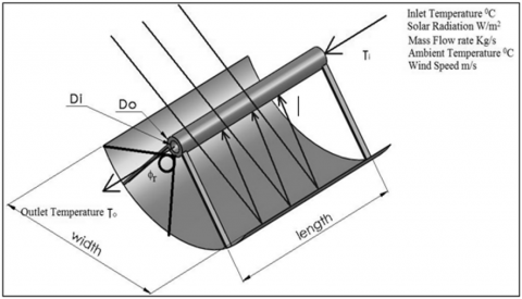
The simulation in this study aims to develop a concept design performance for a power system using a solar parabolic trough as the energy source. This energy source is used to provide heat to a thermal storage system, which is in turn used to provide hot oil to a steam generator. This section focuses on the conceptual performance design for the parabolic trough as the energy source. The basic schematic of the proposed system is shown in Figure 1.
Figure 1. Concept of the parabolic trough
The primary mirror reflectivity, collector absorptance (b), cover gearbox (b), and intercept factor (b) together make up the overall optical efficiency. Eq. (1) expresses the value of the system's overall optical efficiency as:
η(θ)=ρ.(τα)b.γ (1)
The intercept factor is impacted by the impacts of inaccuracies in the concentrating contours, tracking, and receiver movement from the focus, which all result in enlarged or shifted pictures. Biaxial incidence angle modifiers can be used to correct for these issues. However, it varies greatly depending on the collector. Eq. (2) describes the simulation and includes recommended incident angle modifiers (K(θ)Duf).
K(θ)Duf=1-6.74E- .θ2+1.64E-6.θ3–2.51E-8.θ4 (2)
where, θ is in degrees. Eq. (2) is used in the case where the optical efficiency is a function of the angle of incidence. This calculation is made below and is used in the simulation as the modified overall optical efficiency.
ηo,mod(θ)=K(θ)Duf .η(θ) (3)
The absorber tube's convection, radiation, and conduction losses to the surrounding air and to the structure supporting the parabolic trough are what cause the thermal losses. In the current simulation, it was assumed that there would be very little transfer of energy from the support structure to the absorber tube. In addition, it was planned for a glass cover to cover the cylindrical receiver throughout the whole length of the trough. These presumptions were based on actual applications; however, there might be areas where the simulation could be improved in the future.
2.1 Methodology
Solar PTC performance is modeled in ANSYS Workbench version 16 using meteorological and process heat demand data. The goal of the ANSYS Workbench is to offer reliable and user-friendly meshing tools to streamline the mesh creation process. These tools offer the advantages of moderate to high levels of user control and high levels of automation. An examination of the system design parameters and their implications on the various trough configurations' economic competitiveness is provided by the process simulation.
2.2 Heat loss by radiation
For a system with a glass cover, there are two radiation coefficients that must be computed. The first coefficient represents the radiation that travels from the absorber pipe (receiver) to the cover glass. This coefficient is provided by Eq. (4).
$h_r=\frac{\sigma\left(T 2^2+T 1^2\right)(T 2+T 1)}{\frac{1-\varepsilon 1}{\varepsilon 1}+\frac{1}{F 12}+\frac{(1-\varepsilon 2) A 1}{\varepsilon 2 A 2}}$ (4)
where, A1 is the area of the receiver (the absorber pipe), A2 is the area of the cover, T1 is the temperature of the receiver (the absorber pipe), T2 is the temperature of the cover, F12 is the view factor between the receiver and the cover (assumed to be 1), and $\mathcal{E}$ is the Stefan Boltzmann constant, which equals 5.67e-8. It is assumed that the surfaces in this equation are grey with a constant temperature, and are equally exposed to incident energy. The 3D structured mesh of PTC in the present work was designed using a pointwise program. The number of mesh sizes was selected after performing a mesh size independence test. The mesh size independence test acts on five meshes with different mesh sizes to study the change in outlet temperature among the different meshes. The mesh size was gradually and uniformly increased from 633,017.64 cells to 945,619.84 cells. Therefore, the simulation makes an effort to arrive at a reasonable estimation of the average receiver temperature Tr during the evaluation. Consequently, a mesh size was chosen for the current study in order to reduce calculation time without sacrificing result accuracy. The temperature of the receiver and cover must be determined in order to calculate this coefficient, as is evident from Eq. (5). The evaluation length is then iterated a second time to further refine this logical estimate. Eq. (5) yields the expected receiver temperature.
$T_r=T_{i n}+0.25 . S .\left(\frac{\left(a-D_c\right) * l_{\text {eval }}}{m * C p}\right)$ (5)
where, Dc is the receiver cover's diameter, a is the aperture width of the trough, leval is the trough's evaluation length, Tin denotes the intake temperature of the oil, m is the mass flow rate, and Cp is the specific heat.
The cover temperature, or the difference between the receiver temperatures and ambient, is assumed to be 20% higher than ambient in the simulation. The cover temperature is then confirmed in the simulation, and Eq. (6) runs a second iteration of the thermal losses using the changed cover temperature Tc.
Tc=0.2.(Tr-Ta)+Ta (6)
where, Ta is the ambient temperature. The radiation coefficient between the cover and the surrounding air is the second coefficient. Eq. (7) describes this coefficient.
hr,c-a=σ.εc.(Tc2+Ta2)(Tc+Ta) (7)
where, Tc is the cover temperature, Ta is the ambient air temperature, and εcis the emittance of the cover.
The parabolic trough has a positive thermal output Qut, if the oil medium's starting temperature is higher than the exit temperature of the heat transfer fluid (HTF) from the parabolic trough. This useful outcome is provided by Eq. (8).
Qu,t=mf.(hto-hti) (8)
where, hto, hti, and mf are the enthalpies of the heating oil entering and leaving the trough, and mfis the mass flow of the heating oil leaving the trough. On the other hand, if the HTF's temperature is lower than the initial temperature of the oil medium, it cannot provide thermal output. The amount of meaningful gain from energy transmission is defined as the efficiency of the parabolic trough. The area of the parabolic trough is divided by the amount of energy poured into it. Eq. (9) describes how to express this efficiency.
ηtrough=Qu tot/(Idirect.Aa) (9)
where, Aa is the area of the aperture/reflector, Idirect is the direct beam radiation, and Qu,tot is the hourly total usable gain for the trough. The steady-state mathematical model is used to investigate the parabolic trough. The model considers the effects of all thermodynamic losses as well as the performance ratio, the specific heat transfer area, and the specific oil flow rate. The typical key assumptions for the steady-state analysis are shown in Table 1.
Table 1. Typical main input parameters
|
Item |
Value |
|
Reflector type |
Reflectech film mirror |
|
Collector orientation |
N- S |
|
Absorber selective coating |
Solel UVAC Cermet (0.10 @ 400℃) |
|
Collector dimensions |
D2 = 0.066 m D3 = 0.070 m D4 = 0.115 m D5 = 0.121 m |
|
Waperture |
5.59 m |
|
Lcollector |
24 m |
|
Existence of the glass envelope |
No |
|
HTF type |
ABCO |
|
Mass flow rate of collector absorber oil |
1.41 kg/s |
|
HTF flow type |
Pipe flow |
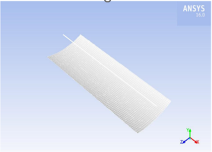
Various researchers have reported numerical studies using the FLUENT-based numerical analysis of a PTC to forecast collector performance. This study determines the distributed temperature in the tube and thermal efficiency during the four seasons of the year. Figure 2 shows modeling of the parabolic trough.
Figure 2. Modeling of the PTC
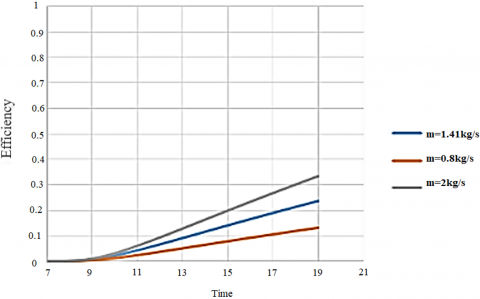
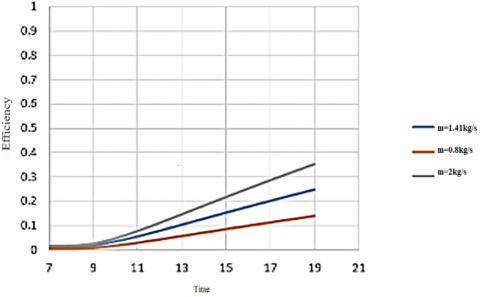
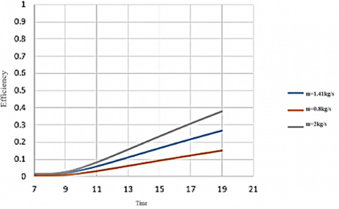
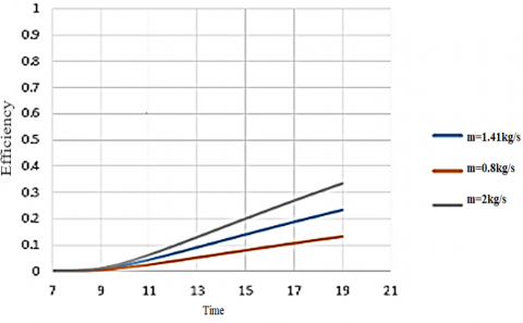
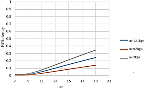
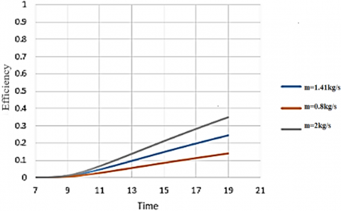
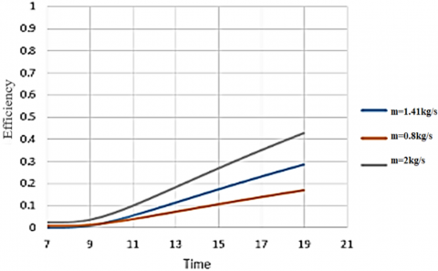
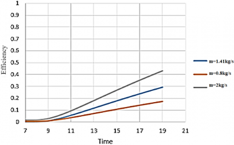
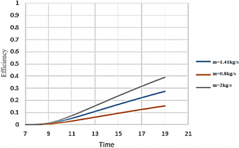
3.1 First season (winter)
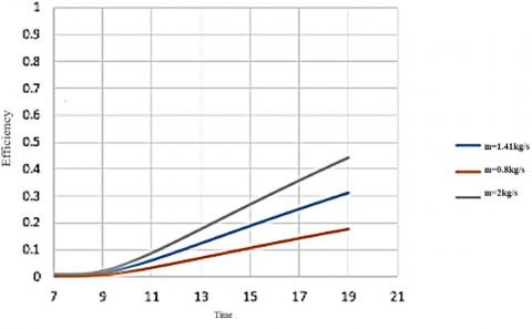
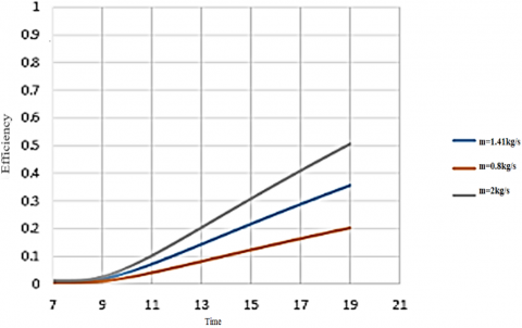
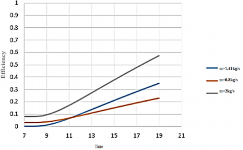
As it was mentioned before, temperature increases more with a lower mass flow rate. On the contrary, it was found that due to the quick rise in temperature caused by the low mass flow rate, the efficiency of the PTC also becomes low. Therefore, calculating the efficiency of the PTC depends on the output temperature of the PTC. Figures 3-9 show the efficiency calculated throughout the week at a mass flow rate of 1.41 Kg/s. As shown on the last day, the efficiency doesn’t exceed 35%. On the other hand, the efficiency reached 50% when the mass flow rate of 2 Kg/s was used, although it is not possible for the efficiency to exceed 40% due to heat losses. Table 2 shows the specifications used for the heat loss using the ANSYS model in January. Experiments were done during the winter, starting from January 15 to January 21. On the first day, the initial temperature entered into the PTC was 19℃, according to the temperature that day at that time. Then, for the next few days, the final temperature reached on a certain day was used as the initial temperature for the following day, taking into consideration the percentage error caused by the decreases in temperatures at night. After almost a week, it was noticed that the temperature in the PTC had become constant. This means that as the temperature increases, the efficiency increases and varies from country to country. It is the same in the other seasons of the year.
Figure 3. Thermal efficiency on January 15th
Figure 4. Thermal efficiency on January 16th
Figure 5. Thermal efficiency on January 17th
Figure 6. Thermal efficiency on January 18th
Figure 7. Thermal efficiency on January 19th
Figure 8. Thermal efficiency on January 20th
Figure 9. Thermal efficiency on January 21st
Table 2. Heat loss specifications using the ANSYS model in January
|
Parameter |
Value |
|
Inlet temperature (K) |
292K, 353K |
|
Beam radiation (W/m2) |
737, 742, 727, 732, 626, 731, 632 |
|
Atmospheric air pressure |
1 atm |
|
Fluid for heat transfer |
VP-1 |
|
Flow rate of HTF |
1.41(kg/s) |
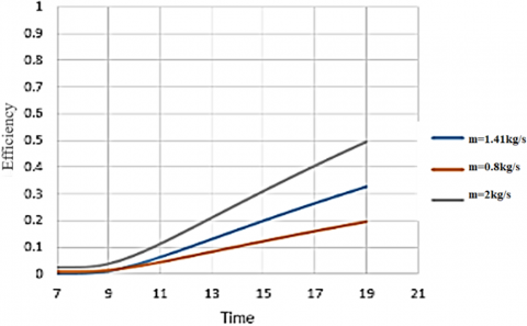
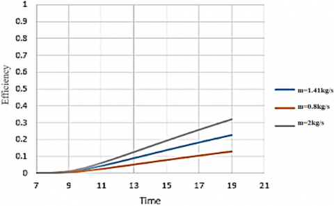
3.2 Second season (spring)
Figures 10-17 show the calculated efficiency of the pipe through the week during which the heating process took place. As shown, the efficiency reached 38% on the last day. Therefore, it can be concluded that the efficiency is relatively higher in April (spring) than in January (winter). Table 3 shows the specifications used for the heat loss ANSYS model in April.
Table 3. Heat loss specifications using the ANSYS model in April
|
Parameter |
Value |
|
Inlet temperature (K) |
303K, 403K |
|
Beam radiation (W/m2) |
736, 742, 721, 727, 703, 698, 656, 742 |
|
Atmospheric air pressure |
1 atm |
|
Fluid for heat transfer |
VP-1 |
|
Flow rate of HTF |
1.41(kg/s) |
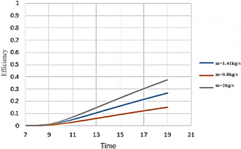
3.3 Third season (summer)
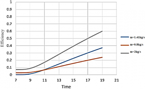
Due to the fast increase in the oil’s temperature, the thermal efficiency was also rapidly increasing. On the first day, the thermal efficiency obtained was 25%. Then on the third, the thermal efficiency obtained was 34%. Finally, on the last day, the average thermal efficiency obtained was 38%, as shown in Figures 18-20. Table 4 shows the specifications used for the heat loss ANSYS model in July.
Figure 10. Thermal efficiency on April 15th
Figure 11. Thermal efficiency on April 16th
Figure 12. Thermal efficiency on April 17th
Figure 13. Thermal efficiency on April 18th
Figure 14. Thermal efficiency on April 19th
Figure 15. Thermal efficiency on April 20th
Figure 16. Thermal efficiency on April 21st
Figure 17. Thermal efficiency on April 22nd
Figure 18. Thermal efficiency on July 15th
Figure 19. Thermal efficiency on July 16th
Figure 20. Thermal efficiency on July 17th
Table 4. Heat loss specifications using the ANSYS model in July
|
Parameter |
Value |
|
Inlet temperature (K) |
310, 425 |
|
Beam radiation (W/m2) |
626, 593, 627 |
|
Atmospheric air pressure |
1 atm |
|
Fluid for heat transfer |
VP-1 |
|
Flow rate of HTF |
1.41(kg/s) |
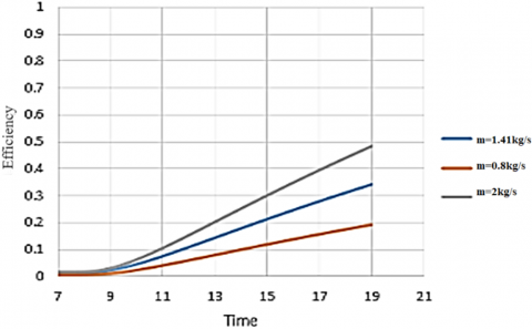
3.4 Fourth season (fall)
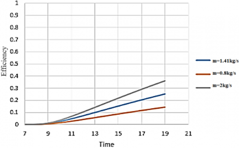
Due to the decrease in temperature, the thermal efficiency obtained in October was about 34% which is less than the thermal efficiency obtained in July, as shown in Figures 21-26. Table 5 shows the specifications used for the heat loss ANSYS model in October.
Figure 21. Thermal efficiency on October 15th
Figure 22. Thermal efficiency on October 16th
Figure 23. Thermal efficiency on October 17th
Figure 24. Thermal efficiency on October 18th
Figure 25. Thermal efficiency on October 19th
Figure 26. Thermal efficiency on October 20th
Table 5. Heat loss specifications using the ANSYS model in October
|
Parameter |
Value |
|
Inlet temperature (K) |
300, 403 |
|
Beam radiation (W/m2) |
541, 530, 534, 532, 509, 508, 466 |
|
Atmospheric air pressure |
1 atm |
|
Fluid for heat transfer |
VP-1 |
|
Flow rate of HTF |
1.41(kg/s) |
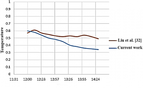
Figures 27 and 28 show the comparison between the present results and the experimental results of Liu et al. [32]. The results of the authors were expressed by the relationship between the efficiency of the parabolic trough and the solar flux and the HTF mass flow rate. The main parameters of the parabolic trough and the comparison conditions used are shown in Table 6.
Figure 27. Comparison between the calculated efficiency of the parabolic trough and the values measured by Liu et al. [32]
Figure 28. Comparison between the calculated temperature of the parabolic trough and the values measured by Liu et al. [32]
Table 6. Parameters of the parabolic trough and the comparison conditions used by Liu et al. [32]
|
Item |
Value |
|
Area (m2) |
30 |
|
Collector aperture (m) |
2.5 |
|
Length (m) |
12 |
|
Rim angle (o) |
31 |
|
Focal distance (m) |
2.25 |
|
Concentration ratio |
38 |
|
Inner diameter of the receiver (m) |
0.0605 |
|
Outer diameter of the receiver (m) |
0.0635 |
|
Inner diameter of the glass envelope (m) |
0.099 |
|
Outer diameter of the glass envelope (m) |
0.102 |
|
Mirror reflection coefficient |
0.90 |
|
Glass transmission coefficient |
0.92 |
|
Absorber absorption coefficient |
>0.9 |
|
Glass tube conductivity coefficient (W/(m K)) |
40 |
|
Absorber emissive coefficient |
0.08@100℃ 0.20@400℃ |
|
Absorber tube conductivity coefficient (W/(m K)) |
1.2 |
|
The direction of the parabolic trough tracking axis |
East-west |
|
Insolation (w/m2) |
200:900 |
|
HTF mass flow rate (Kg/s) |
1.41 |
This study investigated the numerical analysis of a PTC using FLUENT to predict the performance of the PTC. The study figured out how to divide the heat efficiency of the tube among the four different seasons. Calculating the efficiency of the PTC depends on the output temperature of the PTC. In the first season, the efficiency did not exceed 35%, but it reached 38% on the last day of the second season. On the last day of the third season, the average thermal efficiency obtained was 38%. Finally, due to the decrease in temperature in the fourth season, the thermal efficiency obtained in October was about 34%. Finally, this study compared the results with those of previous studies, which shows good agreement with a maximum difference of about 2%. The impact of heat loss on the collector efficiency was also investigated. Point-wise software was employed in this study to create a 3D structured mesh of the PTC. Future research will advance upon this study by investigating the possibility of applying renewable energy (e.g., solar and wind energy) as the main energy source for the district cooling technology. More work is also being done to simulate 3D portions of receivers with varied shapes and flow through the vacuum jacket with gases at different pressures and mass flow rates.
[1] Hamada, M.A., Ehab, A., Khalil, H., Al-Sood, A., Kandeal, A. W., Sharshir, S. (2022). Factors affecting the performance enhancement of a parabolic trough collector utilizing mono and hybrid nanofluids: A mini review of recent progress and prospects. Journal of Contemporary Technology and Applied Engineering, 1(1): 49-61. https://doi.org/10.21608/jctae.2022.152256.1007
[2] Osorio, J.D., Rivera-Alvarez, A. (2022). Influence of the concentration ratio on the thermal and economic performance of parabolic trough collectors. Renewable Energy, 181: 786-802. https://doi.org/10.1016/j.renene.2021.09.040
[3] Wang, Q., Shen, B., Huang, J., Yang, H., Pei, G., Yang, H. (2021). A spectral self-regulating parabolic trough solar receiver integrated with vanadium dioxide-based thermochromic coating. Applied Energy, 285: 116453. https://doi.org/10.1016/j.apenergy.2021.116453
[4] Kalogirou, S.A. (2004). Solar thermal collectors and applications. Progress in Energy and Combustion Science, 30(3): 231-295. https://doi.org/10.1016/j.pecs.2004.02.001
[5] Odeh, S.D., Morrison, G.L., Behnia, M. (2018). Modelling of parabolic through direct steam generation solar collectors. Solar Energy, 62(6): 395-406. https://doi.org/10.1016/S0038-092X(98)00031-0
[6] Aly, N.H., Karameldin, A., Shamloul, M.M. (1999). Modelling and simulation of steam jet ejectors. Desalination, 123(1): 1-8. https://doi.org/10.1016/S0011-9164(99)00053-3
[7] Quaschning, V., Kistner, R., Ortmanns, W. (2002). Influence of direct normal irradiance variation on the optimal parabolic trough field size: A problem solved with technical and economical simulations. Journal of Solar Energy Engineering, 124(2): 160-164. https://doi.org/10.1115/1.1465432
[8] Odeh, S.D. (2003). Unified model of solar thermal electric generation systems. Renewable Energy, 28(5): 755-767. https://doi.org/10.1016/S0960-1481(02)00044-7
[9] Odeh, S.D., Behnia, M., Morrison, G.L. (2003). Performance evaluation of solar thermal electric generation systems. Energy Conversion and Management, 44(15): 2425-2443. https://doi.org/10.1016/S0196-8904(03)00011-6
[10] Stuetzle, T., Blair, N., Mitchell, J.W., Beckman, W.A. (2004). Automatic control of a 30 MWe SEGS VI parabolic trough plant. Solar Energy, 76(1-3): 187-193. https://doi.org/10.1016/j.solener.2003.01.002
[11] Dudley, J.M., Genty, G., Coen, S. (2006). Supercontinuum generation in photonic crystal fiber. Reviews of Modern Physics, 78(4): 1135. https://doi.org/10.1103/RevModPhys.78.1135
[12] Lüpfert, E., Pottler, K., Ulmer, S., Riffelmann, K.J., Neumann, A., Schiricke, B. (2007). Parabolic trough optical performance analysis techniques. Journal of Solar Energy Engineering, 129(2): 147-152. https://doi.org/10.1115/1.2710249
[13] Yang, Y., Cui, Y., Hou, H., Guo, X., Yang, Z., Wang, N. (2008). Research on solar aided coal-fired power generation system and performance analysis. Science in China Series E: Technological Sciences, 51(8): 1211-1221. https://doi.org/10.1007/s11431-008-0172-z
[14] Roesle, M., Coskun, V., Steinfeld, A. (2011). Numerical analysis of heat loss from a parabolic trough absorber tube with active vacuum system. Journal of Solar Energy Engineering, 133(3): 031015. https://doi.org/10.1115/1.4004276
[15] Wagner, M.J., Gilman, P. (2011). Technical manual for the SAM physical trough model (No. NREL/TP-5500-51825). National Renewable Energy Lab. (NREL), Golden, CO (United States). https://doi.org/10.2172/1016437
[16] Laird, A.D., Spiegler, K.S. (1980). Principles of Desalination. Academic Press.
[17] Akbarimoosavi, S.M., Yaghoubi, M. (2014). 3D Thermal-structural analysis of an absorber tube of a parabolic trough collector and the effect of tube deflection on optical efficiency. Energy Procedia, 49: 2433-2443. https://doi.org/10.1016/j.egypro.2014.03.258
[18] Zadeh, P.M., Sokhansefat, T., Kasaeian, A.B., Kowsary, F., Akbarzadeh, A. (2015). Hybrid optimization algorithm for thermal analysis in a solar parabolic trough collector based on nanofluid. Energy, 82: 857-864. https://doi.org/10.1016/j.energy.2015.01.096
[19] He, Y.L., Xiao, J., Cheng, Z.D., Tao, Y.B. (2011). A MCRT and FVM coupled simulation method for energy conversion process in parabolic trough solar collector. Renewable Energy, 36(3): 976-985. https://doi.org/10.1016/j.renene.2010.07.017
[20] Cheng, Z.D., He, Y.L., Xiao, J., Tao, Y.B., Xu, R.J. (2010). Three-dimensional numerical study of heat transfer characteristics in the receiver tube of parabolic trough solar collector. International Communications in Heat and Mass Transfer, 37(7): 782-787. https://doi.org/10.1016/j.icheatmasstransfer.2010.05.002
[21] Mwesigye, A., Bello-Ochende, T., Meyer, J.P. (2014). Heat transfer and thermodynamic performance of a parabolic trough receiver with centrally placed perforated plate inserts. Applied Energy, 136: 989-1003. https://doi.org/10.1016/j.apenergy.2014.03.037
[22] Pigozzo Filho, V.C., de Sá, A.B., Passos, J.C., Colle, S. (2014). Experimental and numerical analysis of thermal losses of a parabolic trough solar collector. Energy Procedia, 57: 381-390. https://doi.org/10.1016/j.egypro.2014.10.191
[23] Zhang, L., Gong, M., Peng, L.M. (2013). Microstructure and strengthening mechanism of a thermomechanically treated Mg–10Gd–3Y–1Sn–0.5 Zr alloy. Materials Science and Engineering: A, 565: 262-268. https://doi.org/10.1016/j.msea.2012.12.051
[24] Zhang, L., Wang, W., Yu, Z., Fan, L., Hu, Y., Ni, Y., Fan, J., Cen, K. (2012). An experimental investigation of a natural circulation heat pipe system applied to a parabolic trough solar collector steam generation system. Solar Energy, 86(3): 911-919. https://doi.org/10.1016/j.solener.2011.11.020
[25] Xiao, X., Zhang, P., Shao, D.D., Li, M. (2014). Experimental and numerical heat transfer analysis of a V-cavity absorber for linear parabolic trough solar collector. Energy Conversion and Management, 86: 49-59. https://doi.org/10.1016/j.enconman.2014.05.001
[26] Valenzuela, L., López-Martín, R., Zarza, E. (2014). Optical and thermal performance of large-size parabolic-trough solar collectors from outdoor experiments: A test method and a case study. Energy, 70: 456-464. https://doi.org/10.1016/j.energy.2014.04.016
[27] Kumar, D., Kumar, S. (2017). Simulation analysis of overall heat loss coefficient of parabolic trough solar collector at computed optimal air gap. Energy Procedia, 109: 86-93. https://doi.org/10.1016/j.egypro.2017.03.057
[28] Khosravi, A., Malekan, M., Assad, M.E. (2019). Numerical analysis of magnetic field effects on the heat transfer enhancement in ferrofluids for a parabolic trough solar collector. Renewable Energy, 134: 54-63. https://doi.org/10.1016/j.renene.2018.11.015
[29] Al-Rashed, A.A., Alnaqi, A.A., Alsarraf, J. (2021). Numerical investigation and neural network modeling of the performance of a dual-fluid parabolic trough solar collector containing non-Newtonian water-CMC/Al2O3 nanofluid. Sustainable Energy Technologies and Assessments, 48: 101555. https://doi.org/10.1016/j.seta.2021.101555
[30] Shaker, B., Gholinia, M., Pourfallah, M., Ganji, D.D. (2022). CFD analysis of Al2O3-syltherm oil Nanofluid on parabolic trough solar collector with a new flange-shaped turbulator model. Theoretical and Applied Mechanics Letters, 12(2): 100323. https://doi.org/10.1016/j.taml.2022.100323
[31] Abdelrazik, A.S., Osama, A., Allam, A.N., Shboul, B., Sharafeldin, M.A., Elwardany, M., Masoud, A.M. (2023). ANSYS-fluent numerical modeling of the solar thermal and hybrid photovoltaic-Based solar harvesting systems. Journal of Thermal Analysis and Calorimetry, 148(21): 11373-11424. https://doi.org/10.1007/s10973-023-12509-2
[32] Liu, Q., Wang, Y., Gao, Z., Sui, J., Jin, H., Li, H. (2010). Experimental investigation on a parabolic trough solar collector for thermal power generation. Science in China Series E: Technological Sciences, 53(1): 52-56. https://doi.org/10.1007/s11431-010-0021-8