Alaa Falih Mahdi*![]() | Hussein K. Asker
| Hussein K. Asker![]() | Inaam R. Al-Saiq
| Inaam R. Al-Saiq![]()
© 2024 The authors. This article is published by IIETA and is licensed under the CC BY 4.0 license (http://creativecommons.org/licenses/by/4.0/).
OPEN ACCESS
To illustrate the dynamics of the COVID-19, we have introduced a mathematical model called PSITPS and shown the effect of protection (vaccination) after treatment. The proposed model solution's positivity, boundedness, existence, and uniqueness are analyzed. The model's possible equilibrium points were also identified, and the NextGeneration Matrix was employed to calculate the Basic Reproduction Number $\mathcal{R}_0$. This study dealt with the stability of equilibrium points at the local and global levels under specific conditions. The Disease-Free Equilibrium point is locally asymptotically stable when $\mathcal{R}_0<1$; otherwise, it's unstable. By creating the Lyapunov function, we showed that the endemic equilibrium points are globally stable. In this work, we conducted numerical simulations of the model using true data from the COVID-19 epidemic in Najaf. It is a city where religious events abound with large gatherings, which lead to violation of health instructions to avoid infection with COVID-19. The simulation showed that protection (vaccination) after treating the infected had a substantial effect on mitigating the spread of COVID-19. The paper highlights the role of vaccination as a protective measure in effectively controlling the transmission of COVID-19 and mitigating the incidence of illness within the community.
basic reproduction number $\mathcal{R}_0$, COVID-19, deterministic model, equilibrium points, numerical simulation, stability
In 1760, Daniel Bernoulli proposed a resolution to his mathematical model pertaining to smallpox [1], and modeling infectious diseases are still as important today. The use of mathematical models to research epidemic causes and effects, however, did not gain widespread acceptance until the 20th century. The first model was created in 1927 by Kermack and McKendrick and is known as the SIR model [2]. This model classifies the population into three distinct groups: susceptible, infected, and removed. The model takes into account group interactions that are based on rates of disease transmission and eradication as well as a constant total population.
The individuals that have been removed can be employed to transform a population size that is dependent on time into a population size that is constant, even though in some models they are used to represent vaccinated individuals. There are advanced modifications of the SIR model, such as the SIRD, SEIR, and SEIRD models [3-5]. Hundreds of viruses comprise the coronavirus family. The SARS-CoV, or severe acute respiratory syndrome coronavirus, was identified in November 2002. In September 2012, researchers identified the Middle East respiratory syndrome coronavirus (MERS-CoV). Both were linked to serious respiratory conditions and high mortality rates [6, 7]. The identification of SARS-CoV-2, a novel coronavirus associated with severe acute respiratory syndrome, has led to the emergence of a contagious disease often referred to as coronavirus disease 2019 (COVID-19) [8].
In Wuhan, China, the virus was initially identified and reported in December 2019. SARS-CoV-2 is a very contagious virus and rapidly spreads around the world [9]. More than 2.1 million COVID-19 cases have been confirmed by the WHO, together with 142,229 fatalities [10]. Iraq is one of the nations that has had significant repercussions as a result of the viral outbreak. On February 25, 2020, the first recorded case of COVID-19 was confirmed in the Najaf governorate for an Iranian student who came from Iran [11], supported by four cases from one family in the Kirkuk governorate on February 26, 2020. All of these cases had a travel history to Iran [12].
COVID-19 cases in total from January 3, 2020, to December 8, 2022, is 2,463,296 confirmed cases with 25,363 deaths in Iraq [13]. While in Najaf Governorate, the cumulative total of COVID-19 cases from March 31, 2020, to May 9, 2022, is 95,147 confirmed cases with 728 deaths [14]. However, according to available data, the cumulative count of COVID-19 cases in Najaf from January 1, 2021, to December 31, 2021, amounted to 68,394, resulting in 397 fatalities [15].
Many studies have been performed on the dynamics of COVID-19.
Abidemi et al. [16] offered a carefully designed deterministic compartmental model to explore the influence of several pharmacological and non-pharmacological control methods on COVID-19 population dynamics in Malaysia. The influence of different control combination techniques incorporating the use of safeguarding oneself, tracking of contacts and laboratory tests, and treatment control measures on disease transmission is demonstrated using numerical simulations. According to numerical simulations, the use of each technique analysed can dramatically lower both the prevalence and incidence of COVID-19 within the general community.
Lobato et al. [17] proposed a technique for parameter estimation in compartmental models through the use of a dynamic data segmentation approach. The likelihood of transmission by touch for each wave is represented by a time-dependent function. The findings offer details on the epidemic's features for each nation as well as input for economic and governmental decision-making.
Rida et al. [18] presented a Mathematical SEIAR Model to analyse the transmission dynamics of the ongoing COVID-19 epidemic. Where the population was categorized into five distinct groups, namely susceptible $S(t)$, exposed $E(t)$, symptomatic $I(t)$, asymptomatic $A(t)$, and recovered $R(t)$. The reproduction number $\mathcal{R}_0$ is used to conduct a sensitivity analysis and identify the most important variables from which to calculate the COVID-19 propagation volume. A numerical simulation was given and is based on data to estimate COVID19's worldwide spread.
Mustafa and Ahmad [19] investigated the impact of contaminated objects on a SIRS model, including compartments for vaccination and hospitalization. The model's solutions are shown to be positive and bounded. When the value of the Basic Reproduction Number is below 1, the examination of the Disease-Free Equilibrium point demonstrates its worldwide stability. Studies on the presence and distinctiveness of the Endemic Equilibrium point are conducted when the Basic Reproduction Number surpasses one.
Hamou et al. [20] studied the mathematical modeling of undiscovered new coronavirus infections in Morocco. The model's parameters and undiscovered COVID-19 instances were evaluated using the least squares approach and were discarded. The researchers employed the MATLAB programming language to explore unexplored scenarios in Morocco and confirm projected results.
Salam et al. [21] developed the SIUWR model they previously used and added certain transmission parameters. The model has five compartments called susceptible people S, people who are infected but have no symptoms I, unreported cases of symptomatic infection U, reported infected people with symptoms W, and recovered people R. The calculation of the Basic Reproduction Number and elastic characteristic coefficients was performed at the Equilibrium Points. The stated model's validity was tested by comparing it to some real data that was collected in Iraq and France between January 1st and December 25th, 2021. The results offered some biological interpretations, which may be utilized to help control this epidemic.
Rai [22] proposed a compartmental SVEIDRS Epidemic Model in order to examine the diffusion dynamics associated with COVID-19. The whole population (N) has been split into six compartments in the bio-mathematical model used. S(t) Amount of people who have not been exposed to the virus and have not developed immunity to it. V(t) is the number of people who were immunized against the virus. E(t) Amount of people who have been exposed to the virus but have not exhibited symptoms and are still in the incubation stage. I(t) Amount of people that have previously been exposed to the virus, are exhibiting illness symptoms and can spread the sickness. D(t) Amount of people who died as a result of complications induced by the virus. R(t) Number of people who have recovered from the virus and are immune to it for a set period of time. Examined are the results of vaccination as well as its effectiveness. A sensitivity analysis is conducted to examine the impact of model parameters on the propagation of a disease in the presence of vaccination. The possibility of COVID-19 is decreased, and the spread of the disease is controlled through the use of efficient vaccinations, improvements to healthcare infrastructure, and intentional measures to minimize human-to-human contact.
In a recent study, Mohammed and Khoshnaw [23] developed a mathematical model that incorporates a vaccination compartment. The model employed in this study adopts an equation-based methodology and aims to offer a full comprehension of the dynamics pertaining to vaccination. The present investigation centers on the analysis of empirical evidence derived from officially confirmed cases in the Kurdistan Region of Iraq during the period spanning from July 17, 2021, to January 1, 2022. In this study, the authors utilized MATLAB's computational tools to compare the total number of infected individuals with both model predictions and empirical data. The computational analysis reveals a striking resemblance between the dynamics of model outcomes and the actual, validated instances. The examination of elasticity coefficients provides a comprehensive comprehension of the impact of vaccination on transmission. The results of this model possess the capacity to provide a valuable contribution to the worldwide effort of effectively managing this ailment by offering supplementary recommendations and enhancements.
The authors, Satar and Naji [24] conducted a study whereby they introduced and examined a mathematical framework that effectively represents the transmission dynamics of COVID-19 throughout the population of asymptomatic individuals. A thorough examination was undertaken to analyse every component of the system's solution. A computation was conducted to determine the Equilibrium Points and the Basic Reproduction Number. The researchers performed local stability studies for both the equilibrium state without disease and the equilibrium state with disease present. In contrast to the Castillo-Chavez theorem, which was utilised to examine the global stability of the Disease-Free Equilibrium, a geometric approach was adopted to analyse the global dynamics of the Endemic Equilibrium. The analysis uncovered that the system's transcritical bifurcation occurs when there is an absence of sickness. The confirmation of the findings and the determination of the mechanisms governing the transmission of the disease were accomplished through the use of a numerical simulation, specifically applied to the population of Iraq.
To our knowledge, no model examines the effect of protection (vaccination) after treatment. According to what was mentioned above, we extended the model introduced by Wameko et al. [25] to the PSITPS Model for the COVID-19 epidemic and demonstrated the effect of protection (vaccination) after treatment in Najaf.
The PSITPS Model, which emphasizes post-treatment protection through vaccination, was examined in the context of Najaf, Iraq. Real data from the year 2021, obtained from the Public Health Department and the Statistics Division of the Training and Human Development Centre of the Najaf Health Directorate, Ministry of Health, were utilized to conduct numerical simulations and obtain the corresponding results.
This paper is arranged as follows, in the second Section, the Deterministic Model of COVID-19 is formulated. In the third Section, the model was analysed in terms of its positivity, invariant region, boundedness, existence, and uniqueness. In the fourth and fifth Sections, the Equilibrium Points and the Basic Reproduction Number were determined, and the stability of the Equilibrium Points was discussed, respectively. Also, the numerical results and discussion are mentioned in the sixth Section. Finally, the conclusions are given in Section 7.
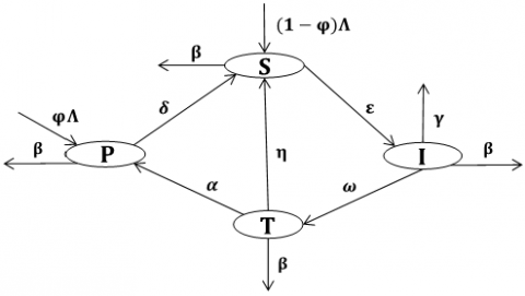
We split the population of Najaf into four classes: at time $t$, the category of individuals denoted as "Protected" $(P(t))$ refers to those who have received vaccination against the illness. On the other hand, the term "Susceptible" $(S(t))$ pertains to those who have not yet been infected by the disease. The term "infected" $(I(t))$ pertains to persons who have contracted an infection, whereas "treated" $(T(t))$ denotes individuals who have effectively undergone a course of therapy. The mathematical model consisting of four differential equations of the first order mentioned below is given, where the flowchart of the model is represented in Figure 1 and each parameter is explained in Table 1.
$\begin{gathered}\frac{d P}{d t}=\varphi \Lambda+\alpha T-(\delta+\beta) P, \\ \frac{d S}{d t}=(1-\varphi) \Lambda+\delta P+\eta T-(\varepsilon+\beta) S, \\ \frac{d I}{d t}=\varepsilon S-(\gamma+\beta+\omega) I, \text { and } \\ \frac{d T}{d t}=\omega I-(\eta+\alpha+\beta) T\end{gathered}$ (1)
where, $\varepsilon=\frac{(1-\vartheta) \pi \theta}{\mathbb{N}} I$ is an effective force of infection, $\vartheta$ is the rate of infection protection efficacy, $\pi$ is the COVID-19 transmission probability rate, $\theta$ is the infection rate per contact, and $\mathbb{N}=P+S+I+T$ with preliminary condition $P(0)=$ $P_0, S(0)=S_0, I(0)=I_0$, and $T(0)=T_0$.
Figure 1. Flowchart of the proposed Model (1)
Table 1. Parameters and its description
|
Parameter Symbol |
Parameter Description |
|
$\Lambda$ |
Birth rate |
|
$\varphi$ |
Already protected rate |
|
$\delta$ |
Rate of loss of protection |
|
$\varepsilon$ |
The effective force of infection |
|
$\omega$ |
Rate of treatment |
|
$\eta$ |
Rate of transmission from T to S |
|
$\alpha$ |
Rate of transmission from T to P |
|
$\gamma$ |
The death rate associated with COVID-19 |
|
$\beta$ |
Natural death rate |
|
$\pi$ |
COVID-19 transmission probability rate |
|
$\theta$ |
Infection rate per contact |
|
$\vartheta$ |
Rate of infection protection efficacy |
|
$\mathbb{N}$ |
Total population size |
This section presents positivity of the solution, the invariant region, and the existence and uniqueness of the solution for Model (1), by applying the technique used by Wameko et al. [25].
3.1 The solution's positivity
The starting condition of the model was assumed to be non-negative, and it is shown that the solution of the model is also positive.
Theorem 1. Solutions of the mathematical Model (1) together with the non-negative preliminary condition $P(0)=P_0, S(0)=S_0, I(0)=I_0$, and $T(0)=T_0$ are always positive; or the classes of model $P(t), S(t), I(t)$, and $T(t)$ are positive for all $t$.
Proof. Positivity of $P(t)$: Consider the first equation given by:
$\frac{d P}{d t}=\varphi \Lambda+\alpha T-(\delta+\beta) P$
After avoiding the positive parts $\varphi \Lambda+\alpha T$ from this equation, reduces to an inequality $\frac{d P}{d t} \geq$ $-(\delta+\beta) P$, and can be described in separable variables form as $\frac{d P}{P} \geq-(\delta+\beta) d t$. Following the integration and application of the initial condition $P(0)=P_0$, the solution can be acquired to be $P(t) \geq$ $P_0 e^{-(\delta+\beta) t}$. Now, since $P_0>0$ and $e^{-(\delta+\beta) t}>0$, it is simple to deduce that:
$P(t) \geq 0, \quad \forall t$.
Positivity of $S(t)$: Consider the second equation given by:
$\frac{d S}{d t}=(1-\varphi) \Lambda+\delta P+\eta T-(\varepsilon+\beta) S$
After avoiding the positive parts $(1-\varphi) \Lambda+\delta P+\eta T$ from this equation, reduces to an inequality $\frac{d S}{d t} \geq-(\varepsilon+\beta) S$ and can be described in separable variables form as $\frac{d S}{S} \geq-(\varepsilon+\beta) d t$. Following the integration and application of the initial condition $S(0)=S_0$, the solution can be acquired to be $S(t) \geq$ $S_0 e^{-(\varepsilon+\beta) t}$. Now, since $S_0>0$ and $e^{-(\varepsilon+\beta) t}>0$, it is simple to deduce that:
$S(t) \geq 0, \quad \forall t$.
Positivity of $I(t)$: By using the same method on the third equation, it can be obtained that:
$I(t) \geq 0, \quad \forall t$.
Positivity of $T(t)$: By using the same method on the fourth equation, it is possible to get that:
$T(t) \geq 0, \quad \forall t$.
We have shown a positive of the solution to the Model (1).
3.2 The invariant region
Theorem 2. The positive solutions of the system of model Eq. (1) are bounded; or, equivalently, the model variables $P(t), S(t), I(t)$, and $T(t)$ are bounded for all $t$. The Invariant Region in which the model solution is bounded has been obtained.
Proof. The entire population $\mathbb{N}$ in the model is given by:
$\mathbb{N}=P+S+I+T$
By deriving $\mathbb{N}$ in both directions with respect to $t$, which leads to
$\frac{d \mathbb{N}}{d t}=\frac{d P}{d t}+\frac{d S}{d t}+\frac{d I}{d t}+\frac{d T}{d t}$ (2)
By replacing model Eqs. (1) with (2), the following is obtained:
$\frac{d \mathbb{N}}{d t}=\Lambda-\beta \mathbb{N}-\gamma I$ (3)
If there are no COVID-19 related death i.e., $\gamma=0$, Eq. (3) becomes
$\frac{d \mathbb{N}}{d t}=\Lambda-\beta \mathbb{N} \Rightarrow \frac{1}{\Lambda-\beta \mathbb{N}} d \mathbb{N} \leq d t$,
and by integration the two sides, the following result is obtained:
$-\frac{1}{\beta} \ln (\Lambda-\beta \mathbb{N}) \leq t+c_1$,
where, $c_1$ is integration constant.
By using antilogarithms and inserting arbitrary constants $c_2=-\beta c_1$ and $B=e^{c_2}$. The generic solution may be written as follows:
$\Lambda-\beta \mathbb{N} \geq B e^{-\mu t}$ (4)
By putting preliminary conditions $\mathbb{N}(0)=\mathbb{N}_0$ in Eq. (4), the next step is obtained:
$B=\Lambda-\beta \mathbb{N}_0$ (5)
By substituting Eqs. (5) for (4), the result is the following:
$\Lambda-\beta \mathbb{N} \geq\left(\Lambda-\beta \mathbb{N}_0\right) e^{-\beta t} \Rightarrow \mathbb{N} \leq \frac{\Lambda}{\beta}-\frac{\left(\Lambda-\beta \mathbb{N}_0\right) e^{-\beta t}}{\beta}$ (6)
Accordingly, $t \rightarrow \infty$ in Eq. (6), the total population size is $\mathbb{N} \rightarrow \frac{\Lambda}{\beta}$, implying that $0 \leq \mathbb{N} \leq \frac{\Lambda}{\beta}$.
As a result, the model's viable solution set enters and remains in the region $\gamma=\{(P, S, I, T) \in$ $\left.\mathbb{R}_{+}^4: \mathbb{N} \leq \frac{\Lambda}{\beta}\right\}$
Therefore, the Model (1) is sound from an epidemiological and mathematical standpoint.
3.3 The solution's existence and uniqueness
Lemma 1. The solutions of the mathematical Model (1) together with the non-negative preliminary conditions $P(0)>0, S(0)>0, I(0)>0$, and $T(0)>0$ exist in $\mathbb{R}_{+}^4$, i.e., the model's solution for $P(t), S(t), I(t)$, and $T(t)$ exist for all $t$ and will continue to exist in $\mathbb{R}_{+}^4$.
Proof. The expressions on the right-hand side of Eq. (1) can be represented as follows:
$\begin{gathered}g_1(P, S, I, T)=\varphi \Lambda+\alpha T-(\delta+\beta) P \\ g_2(P, S, I, T)=(1-\varphi) \Lambda+\delta P+\eta T-(\varepsilon+\beta) S, \\ g_3(P, S, I, T)=\varepsilon S-(\gamma+\beta+\omega) I, \text { and } \\ g_4(P, S, I, T)=\omega I-(\eta+\alpha+\beta) T\end{gathered}$
Let $Y$ represent the region by Derrick and Grossman Theorem, $Y=\left\{(P, S, I, T) \in \mathbb{R}_{+}^4: \mathbb{N} \leq \frac{\Lambda}{\beta}\right\}$.
If $\frac{\partial g_i}{\partial y_j}, i, j=1,2,3,4$ are bounded and continuous in $Y$, then there is only one solution to the mathematical Model (1).
Also here, $y_1=P, y_2=S, y_3=I$ and $y_4=T$. The continuity and the boundedness are confirmed as follows:
|
For $g_1$: |
For $g_2$: |
|
$\begin{aligned} & \left|\frac{\partial g_1}{\partial P}\right|=|-(\delta+\beta)|<\infty \\ & \left|\frac{\partial g_1}{\partial S}\right|=0<\infty \\ & \left|\frac{\partial g_1}{\partial I}\right|=0<\infty \\ & \left|\frac{\partial g_1}{\partial T}\right|=|\alpha|<\infty\end{aligned}$ |
$\begin{aligned} & \left|\frac{\partial g_2}{\partial P}\right|=|\delta|<\infty \\ & \left|\frac{\partial g_2}{\partial S}\right|=|-(\varepsilon+\beta)|<\infty \\ & \left|\frac{\partial g_2}{\partial I}\right|=\left|-\left(\frac{\pi \theta(1-\vartheta)}{\mathbb{N}} S\right)\right|<\infty \\ & \left|\frac{\partial g_2}{\partial T}\right|=|\eta|<\infty\end{aligned}$ |
|
For $g_3$: |
For $g_4$: |
|
$\begin{aligned} & \left|\frac{\partial g_3}{\partial P}\right|=0<\infty \\ & \left|\frac{\partial g_3}{\partial S}\right|=|\varepsilon|<\infty \\ & \left.\frac{\partial g_3}{\partial I}|=|-(\gamma+\beta+\omega) \right\rvert\,<\infty \\ & \left|\frac{\partial g_3}{\partial T}\right|=0<\infty\end{aligned}$ |
$\begin{aligned} & \left|\frac{\partial g_4}{\partial P}\right|=0<\infty \\ & \left|\frac{\partial g_4}{\partial S}\right|=0<\infty \\ & \left|\frac{\partial g_4}{\partial I}\right|=|\omega|<\infty \\ & \left|\frac{\partial g_4}{\partial T}\right|=|-(\eta+\alpha+\beta)|<\infty\end{aligned}$ |
In consequence, all of the partial derivatives $\frac{\partial g_i}{\partial y_j} ; i, j=1,2,3,4$ exist, bounded and continuous in $Y$.
Subsequently, the model's solution (1) is existing and unique, according to Derrick and Grossman Theorem.
In the coming section, the Equilibrium Points and Basic Reproduction Number $\mathcal{R}_0$ for Model (1) are demonstrated.
4.1 Equilibrium points
4.1.1 Disease-Free Equilibrium $\mathbb{E}_0$
It takes into account the steady state of system (1) to obtain a Disease-Free Equilibrium (DFE), which will be:
$\begin{gathered}\varphi \Lambda+\alpha T-(\delta+\beta) P=0, \\ (1-\varphi) \Lambda+\delta P+\eta T-(\varepsilon+\beta) S=0, \\ \varepsilon S-(\gamma+\beta+\omega) I=0, \\ \omega I-(\eta+\alpha+\beta) T=0\end{gathered}$ (7)
Let $I=0$ and $T=0$ be substituted in Eq. (7), and when those equations are solved for non-infected state variables, the following results are obtained:
When calculating the first equation $\varphi \Lambda+\alpha \mathrm{T}-(\delta+\beta) \mathrm{P}=0$ of Eq. (7), the following formula is obtained:
$P=\frac{\varphi \Lambda}{(\delta+\beta)}$
When calculating the second equation $(1-\varphi) \Lambda+\delta P+\eta T-(\varepsilon+\beta) S=0$ of Eq. (7), the following is obtained:
$S=\frac{(\delta+\beta-\varphi \beta) \Lambda}{\beta(\delta+\beta)}$
Therefore, $\mathbb{E}_0=\left(\frac{\varphi \Lambda}{(\delta+\beta)}, \frac{(\delta+\beta-\varphi \beta) \Lambda}{\beta(\delta+\beta)}, 0,0\right)$.
4.1.2 Endemic Equilibrium point $\mathbb{E}^*$
When the illness continues to exist in the population, the Endemic Equilibrium (EE) takes place. It is obtained by equaling all of the Model's Eq. (1) to zero:
$\begin{gathered}\varphi \Lambda+\alpha T-(\delta+\beta) P=0, \\ (1-\varphi) \Lambda+\delta P+\eta T-(\varepsilon+\beta) S=0 \\ \varepsilon S-(\gamma+\beta+\omega) I=0, \text { and } \\ \omega I-(\eta+\alpha+\beta) T=0\end{gathered}$
From $\varphi \Lambda+\alpha T-(\delta+\beta) P=0$, the next is obtained:
$P^*=\frac{\varphi \Lambda+\alpha T^*}{(\delta+\beta)}$ (8)
From $\varepsilon S-(\gamma+\beta+\omega) I=0$, and $\varepsilon=\frac{(1-\vartheta) \pi \theta}{\mathbb{N}} I$, the following is obtained:
$\left(\frac{(1-\vartheta) \pi \theta}{\mathbb{N}} I\right) S-(\gamma+\beta+\omega) I=0$.
Hence,
$S^*=\frac{\mathbb{N}(\gamma+\beta+\omega)}{(1-\vartheta) \pi \theta}$
From $\omega I-(\eta+\alpha+\beta) T=0$, the following formula is obtained:
$T^*=\frac{\omega I^*}{(\eta+\alpha+\beta)}$ (9)
Substituting $P^*, S^*$, and $T^*$ in $(1-\varphi) \Lambda+\delta P+\eta T-(\varepsilon+\beta) S=0$, the following is obtained
$(1-\varphi) \Lambda+\frac{\delta \varphi \Lambda}{(\delta+\beta)}+\frac{\delta \alpha \omega I^*}{(\delta+\beta)(\eta+\alpha+\beta)}+\frac{\eta \omega I^*}{(\eta+\alpha+\beta)}-(\gamma+\beta+\omega) I^*-\frac{\beta \mathbb{N}(\gamma+\beta+\omega)}{(1-\vartheta) \pi \theta}=0$
$\Rightarrow(1-\varphi) \Lambda+\frac{\delta \varphi \Lambda}{(\delta+\beta)}-\frac{\beta \mathbb{N}(\gamma+\beta+\omega)}{(1-\vartheta) \pi \theta}-\left[(\gamma+\beta+\omega)-\frac{\delta \alpha \omega}{(\delta+\beta)(\eta+\alpha+\beta)}-\frac{\eta \omega}{(\eta+\alpha+\beta)}\right] I^*=0$
$\Rightarrow \frac{\pi \theta(1-\vartheta)(\delta+\beta)(1-\varphi) \Lambda+\pi \theta(1-\vartheta) \delta \varphi \Lambda-\beta \mathbb{N}(\delta+\beta)(\gamma+\beta+\omega)}{\pi \theta(1-\vartheta)(\delta+\beta)}$$-\left\lceil\frac{(\delta+\beta)(\eta+\alpha+\beta)(\gamma+\beta+\omega)-\delta \alpha \omega-\eta \omega(\delta+\beta)}{(\delta+\beta)(\eta+\alpha+\beta)}\right\rceil I^*=0$
$\Rightarrow\left[\frac{(\delta+\beta)(\eta+\alpha+\beta)(\gamma+\beta+\omega)-\delta \alpha \omega-\eta \omega(\delta+\beta)}{(\delta+\beta)(\eta+\alpha+\beta)}\right] I^*$$=\frac{\pi \theta(1-\vartheta)(\delta+\beta)(1-\varphi) \Lambda+\pi \theta(1-\vartheta) \delta \varphi \Lambda-\beta \mathbb{N}(\delta+\beta)(\gamma+\beta+\omega)}{\pi \theta(1-\vartheta)(\delta+\beta)}$
$\Rightarrow I^*=\left(\frac{(\delta+\beta)(\eta+\alpha+\beta)}{(\delta+\beta)(\eta+\alpha+\beta)(\gamma+\beta+\omega)-\delta \alpha \omega-\eta \omega(\delta+\beta)}\right)$$\left(\frac{\pi \theta(1-\vartheta)(\delta+\beta)(1-\varphi) \Lambda+\pi \theta(1-\vartheta) \delta \varphi \Lambda-\beta \mathbb{N}(\delta+\beta)(\gamma+\beta+\omega)}{\pi \theta(1-\vartheta)(\delta+\beta)}\right)$.
Hence,
$I^*=\frac{(\eta+\alpha+\beta)(\pi \theta(1-\vartheta)(\delta+\beta)(1-\varphi) \Lambda+\pi \theta(1-\vartheta) \delta \varphi \Lambda-\beta \mathbb{N}(\delta+\beta)(\gamma+\beta+\omega))}{((\delta+\beta)(\eta+\alpha+\beta)(\gamma+\beta+\omega)-\delta \alpha \omega-\eta \omega(\delta+\beta))(\pi \theta(1-\vartheta))}$
Therefore, $\mathbb{E}^*=\left(\mathrm{P}^*, S^*, I^*, T^*\right)$, where,
$P^*=\frac{\varphi \Lambda+\alpha\left[\frac{\omega}{(\eta+\alpha+\beta)}\left(\frac{(\eta+\alpha+\beta)(\pi \theta(1-\vartheta)(\delta+\beta)(1-\varphi) \Lambda+\pi \theta(1-\vartheta) \delta \varphi \Lambda-\beta \mathbb{N}(\delta+\beta)(\gamma+\beta+\omega))}{((\delta+\beta)(\eta+\alpha+\beta)(\gamma+\beta+\omega)-\delta \alpha \omega-\eta \omega(\delta+\beta))(\pi \theta(1-\vartheta))}\right)\right]}{(\delta+\beta)}$,
$S^*=\frac{\mathbb{N}(\gamma+\beta+\omega)}{(1-\vartheta) \pi \theta}$,
$I^*=\frac{(\eta+\alpha+\beta)(\pi \theta(1-\vartheta)(\delta+\beta)(1-\varphi) \Lambda+\pi \theta(1-\vartheta) \delta \varphi \Lambda-\beta \mathbb{N}(\delta+\beta)(\gamma+\beta+\omega))}{((\delta+\beta)(\eta+\alpha+\beta)(\gamma+\beta+\omega)-\delta \alpha \omega-\eta \omega(\delta+\beta))(\pi \theta(1-\vartheta))}$,
$T^*=\frac{\omega}{(\eta+\alpha+\beta)}\left[\frac{(\eta+\alpha+\beta)(\pi \theta(1-\vartheta)(\delta+\beta)(1-\varphi) \Lambda+\pi \theta(1-\vartheta) \delta \varphi \Lambda-\beta \mathrm{N}(\delta+\beta)(\gamma+\beta+\omega))}{((\delta+\beta)(\eta+\alpha+\beta)(\gamma+\beta+\omega)-\delta \alpha \omega-\eta \omega(\delta+\beta))(\pi \theta(1-\vartheta))}\right]$, respectively.
By substituting T* into Eq. (8), the result is the following:
4.2 The basic reproduction number $\mathcal{R}_0$
The basic reproduction number is the average number of secondary cases caused by a COVID-19 infected person in a completely susceptible community. In this part, we calculated the Basic. Reproduction. Number, the critical quantity that limits the disease's spread. With the help of the NextGeneration Matrix method, we can determine the Basic. Reproduction. Number, which is the spectral radius of the matrix. The final equation of Model (1) reads $\frac{d I}{d t}=\varepsilon S-(\gamma+\beta+\omega) I$, where $(\varepsilon S)$ represents freshly infected groups and $(\gamma+\beta+\omega) I$ represents secondary infected groups. The newly infected individuals are then obtained using the Next-Generation Matrix principle:
$f=[\varepsilon S]$
Since, $\varepsilon=\frac{(1-\vartheta) \pi \theta}{\mathbb{N}} I$, the result is the following:
$f=\left[\left(\frac{(1-\vartheta) \pi \theta}{\mathbb{N}} I\right) S\right]$ (10)
Now, taking the partial. derivative of Eq. (10) with respect to I, the following is obtained:
$F=\left[\left(\frac{(1-\vartheta) \pi \theta}{\mathbb{N}}\right) S\right]$
But, since at DFE $S=\frac{(\delta+\beta-\varphi \beta) \Lambda}{\beta(\delta+\beta)}$, Then function $F$ is written as:
$F=\left[\left(\frac{(1-\vartheta) \pi \theta}{\mathbb{N}}\right)\left(\frac{(\delta+\beta-\varphi \beta) \Lambda}{\beta(\delta+\beta)}\right)\right]$
Since, $\mathbb{N} \leq \frac{\Lambda}{\beta}$, the next is obtained:
$F=\left[\frac{\pi \theta(1-\vartheta)(\delta+\beta-\varphi \beta)}{(\delta+\beta)}\right]$ (11)
To get the matrix $v$, which is the secondary infected group:
$v=(\gamma+\beta+\omega) I$. (12)
Taking the partial derivative of Eq. (12) with respect to $I$, the following is obtained:
$V=(\gamma+\beta+\omega)$
By taking inverse $V$, the next is obtained:
$V^{-1}=\left[\frac{1}{(\gamma+\beta+\omega)}\right]$ (13)
By multiplying Eqs. (11) with (13), the result is the following:
$F V^{-1}=\left[\frac{\pi \theta(1-\vartheta)(\delta+\beta-\varphi \beta)}{(\delta+\beta)(\gamma+\beta+\omega)}\right]$ (14)
The basic reproduction number $\mathcal{R}_0$, is referred to as the spectral radius of the Matrix $F V^{-1}$. It is outlined below:
$\rho\left(F V^{-1}\right)=\left[\frac{\pi \theta(1-\vartheta)(\delta+\beta-\varphi \beta)}{(\delta+\beta)(\gamma+\beta+\omega)}\right]$
Therefore, $\mathcal{R}_0=\frac{\pi \theta(1-\vartheta)(\delta+\beta-\varphi \beta)}{(\delta+\beta)(\gamma+\beta+\omega)}$.
Lemma 2. The Endemic Equilibrium $\mathbb{E}^*$ of the Model (1) exists and no Endemic Equilibrium otherwise.
Proof. For the disease to be endemic $\frac{d \mathrm{I}}{d t}>0$ must hold.
That is: $\varepsilon S-(\gamma+\beta+\omega) I>0 \Rightarrow(\gamma+\beta+\omega) I<\varepsilon S$
Since, $\varepsilon=\frac{(1-\vartheta) \pi \theta}{\mathbb{N}} \mathrm{I}$, the next is obtained:
$(\gamma+\beta+\omega) I<\left(\frac{(1-\vartheta) \pi \theta}{\mathbb{N}} I\right) S$
Taking use of the fact that $S<S_1$ where $S_1$ is the total amount of susceptible individuals at DFE:
$\Rightarrow(\beta+\gamma+\omega) I<\left(\frac{(1-\vartheta) \pi \theta}{\mathbb{N}} I\right) S_1$
Divide both sides by $(\beta+\gamma+\omega) \mathrm{I}$, the result is the following:
$1<\left(\frac{(1-\vartheta) \pi \theta}{\mathbb{N}(\gamma+\beta+\omega)}\right) S_1$
Since, $\mathrm{S}_1=\frac{(\delta+\beta-\varphi \beta) \Lambda}{\beta(\delta+\beta)}$, the following is obtained:
$1<\left(\frac{(1-\vartheta) \pi \theta}{\mathbb{N}(\gamma+\beta+\omega)}\right)\left(\frac{(\delta+\beta-\varphi \beta) \Lambda}{\beta(\delta+\beta)}\right)$
Since, $\mathbb{N}=\frac{\Lambda}{\beta}$, the next step is obtained:
$1<\left(\frac{\pi \theta(1-\vartheta)(\delta+\beta-\varphi \beta)}{(\delta+\beta)(\gamma+\beta+\omega)}\right)$
Hence, $1<\mathcal{R}_0$.
Therefore, when $\mathcal{R}_0>1$, a unique Endemic Equilibrium exists.
5.1 Stability of Disease-Free Equilibrium
5.1.1 Local stability of the Disease-Free Equilibrium
Proposition 1. If $\mathcal{R}_0<1$ Then the Disease-Free Equilibrium point is locally asymptotically- stable, and unstable if $\mathcal{R}_0>1$.
Proof. By following the approach outlined by Das [26], the proposition will be proved.
$J=\left[\begin{array}{cccc}-(\delta+\beta) & 0 & 0 & \alpha \\ \delta & -\left(\beta+\frac{(1-\vartheta) \pi \theta}{\mathbb{N}} I\right) & -\left(\frac{(1-\vartheta) \pi \theta}{\mathbb{N}}\right) S & \eta \\ 0 & \frac{(1-\vartheta) \pi \theta}{\mathbb{N}} I & \frac{(1-\vartheta) \pi \theta}{\mathbb{N}} S-(\gamma+\omega+\beta) & 0 \\ 0 & 0 & \omega & -(\eta+\alpha+\beta)\end{array}\right]$ (15)
$J_{\mathbb{E}_0}=\left[\begin{array}{cccc}-(\delta+\beta) & 0 & 0 & \alpha \\ \gamma & -\beta & -\frac{\pi \theta(1-\vartheta)(\delta+\beta-\varphi \beta)}{(\delta+\beta)} & \eta \\ 0 & 0 & \frac{\pi \theta(1-\vartheta)(\delta+\beta-\varphi \beta)}{(\delta+\beta)}-(\gamma+\beta+\omega) & 0 \\ 0 & 0& \omega & -(\eta+\alpha+\beta)\end{array}\right]$ (16)
The Jacobean Matrix is calculated at the DFE. $\mathbb{E}_0$, and the result is: $\operatorname{det}\left(J_{\mathbb{E}_0}-\lambda I\right)=0$, where $\lambda$ is eigenvalue, and $I=\left[\begin{array}{llll}1 & 0 & 0 & 0 \\ 0 & 1 & 0 & 0 \\ 0 & 0 & 1 & 0 \\ 0 & 0 & 0 & 1\end{array}\right]$, the next step is obtained:
$\left|\begin{array}{cccc}-(\delta+\beta)-\lambda & 0 & 0 & \alpha \\ \delta & -\beta-\lambda & -\frac{\pi \theta(1-\vartheta)(\delta+\beta-\varphi \beta)}{(\delta+\beta)} & \eta \\ 0 & 0 & \frac{\pi \theta(1-\vartheta)(\delta+\beta-\varphi \beta)}{(\delta+\beta)}-(\gamma+\beta+\omega)-\lambda & 0 \\ 0 & 0 & \omega & -(\eta+\alpha+\beta)-\lambda\end{array}\right|=0$
$\Rightarrow(-(\beta+\delta)-\lambda)(-\beta-\lambda)\left(\frac{\pi \theta(1-\vartheta)(\delta+\beta-\varphi \beta)}{(\delta+\beta)}-(\beta+\omega+\gamma)-\lambda\right)(-(\beta+\eta+\alpha)-\lambda)=0$
Thus, the eigenvalues are $\lambda_1=-(\beta+\delta), \lambda_2=-\beta, \lambda_3=\frac{\pi \theta(1-\vartheta)(\delta+\beta-\varphi \beta)}{(\delta+\beta)}-(\beta+\omega+\gamma)$, and $\lambda_4=$ $-(\beta+\eta+\alpha)$
Hence, $\lambda_1, \lambda_2$, and $\lambda_4$ are negative, and $\lambda_3$ is negative if $\mathcal{R}_0<1$.
As a result, the Disease-Free Equilibrium point is locally asymptotically stable.
5.1.2 Global stability of the Disease-Free Equilibrium
This section utilises the methodology outlined by Kamgang and Sallet [27] to analyse the global stability of the DFE.
The equations given in Model (1) are expressed in the following manner:
$\begin{gathered}\frac{d X_s}{d t}=M\left(X_s-X_{D F E, s}\right)+M_1 X_i, \\ \frac{d X_i}{d t}=M_2 X_i .\end{gathered}$
where,
$M=\left[\begin{array}{ll}\frac{\partial g_1}{\partial P} & \frac{\partial g_1}{\partial S} \\ \frac{\partial g_2}{\partial P} & \frac{\partial g_2}{\partial S}\end{array}\right], M_1=\left[\begin{array}{ll}\frac{\partial g_1}{\partial I} & \frac{\partial g_1}{\partial T} \\ \frac{\partial g_2}{\partial I} & \frac{\partial g_2}{\partial T}\end{array}\right]$, and $M_2=\left[\begin{array}{ll}\frac{\partial g_3}{\partial I} & \frac{\partial g_3}{\partial T} \\ \frac{\partial g_4}{\partial I} & \frac{\partial g_4}{\partial T}\end{array}\right]$,
such that
$\begin{gathered}g_1(P, S, I, T)=\varphi \Lambda+\alpha T-(\delta+\beta) P, \\ g_2(P, S, I, T)=(1-\varphi) \Lambda+\delta P+\eta T-(\varepsilon+\beta) S, \\ g_3(P, S, I, T)=\varepsilon S-(\gamma+\beta+\omega) I, \\ g_4(P, S, I, T)=\omega I-(\eta+\alpha+\beta) T .\end{gathered}$
The vector corresponding to the transmitting classes is $X_i$, and the vector corresponding the nontransmitting class is $X_s$.
If $M$ has negative. eigenvalues, and $M_2$ is a Metzler Matrix, meaning that its off-diagonal elements do not have negative values, then the DFE is globally asymptotically stable.
For the Model Eq. (1), we have $X_s=(P, S)^t$, and $X_i=(I, T)^t$, where a transposition of the matrix is indicated by the superscript $t$.
It is necessary to confirm that $M_2$ is a Metzler Matrix, and that the matrix $M$ for non-transmitting classes indeed has negative eigenvalues.
The next is obtained from the Model's Eq. (1) for non-transmitting classes:
$M=\left[\begin{array}{cc}-(\delta+\beta) & 0 \\ \delta & -(\varepsilon+\beta)\end{array}\right]$
The eigenvalues are obtained from the matrix $M$ above, $\lambda_1=-(\delta+\beta)$, and $\lambda_2=-(\varepsilon+\beta)$, all of them are real and negative.
Consequently, the system must be $\frac{d X_s}{d t}=M\left(X_s-X_{D F E, s}\right)+M_1 X_i$ at DFE is locally and globally asymptotically stable if $M_2$ is Metzler Matrix.
Rearranging in the right way yields:
$\begin{gathered}M_2=\left[\begin{array}{cc}\left(\frac{\pi \theta(1-\vartheta)}{\mathbb{N}} S-(\gamma+\beta+\omega)\right. & 0 \\ \omega & -(\eta+\alpha+\beta)\end{array}\right], \\ M_1=\left[\begin{array}{cc}0 & \alpha \\ -\left(\frac{\pi \theta(1-\vartheta)}{\mathbb{N}} S\right. & \eta\end{array}\right], \\ X_s-X_{D F E, s}=\left(\begin{array}{c}P-\frac{\varphi \Lambda}{(\delta+\beta)} \\ S-\frac{(\delta+\beta-\varphi \beta) \Lambda}{\beta(\delta+\beta)}\end{array}\right)\end{gathered}$
$M_2$ is a Metzler Matrix because it has non-negative off-diagonal elements.
Consequently, the DFE is asymptotically globally stable.
5.2 Stability of the Endemic Equilibrium
5.2.1 Global stability of the Endemic Equilibrium
Theorem 3. The Endemic. Equilibrium points of the Model (1) are globally asymptotically stable in $Y$ if $\mathcal{R}_0>1$.
Proof. This theorem can be proved using the method described by Tilahun et al. [28].
The Lyapunov function is utilized as follows:
$\mathcal{L}\left(P^*, S^*, I^*, T^*\right)=\left(P-P^*-P^* \ln (P)\right)+\left(S-S^*-S^* \ln (S)\right)+\left(I-I^*-I^* \ln (I)\right)+\left(T-T^*-T^* \ln (T)\right)$
By derivative $\mathcal{L}$ with respect to $t$, the next step is obtained:
$\frac{d \mathcal{L}}{d t}=\left(1-\frac{P^*}{P}\right) \frac{d P}{d t}+\left(1-\frac{S^*}{S}\right) \frac{d S}{d t}+\left(1-\frac{I^*}{I}\right) \frac{d I}{d t}+\left(1-\frac{T^*}{T}\right) \frac{d T}{d t}$
By substituting Model (1) into the above step, the following is obtained:
$\begin{aligned} & \frac{d \mathcal{L}}{d t}=\left(1-\frac{P^*}{P}\right)(\varphi \Lambda+\alpha T-(\delta+\beta) P)+\left(1-\frac{S^*}{S}\right)((1-\varphi) \Lambda+\delta P+\eta T-(\varepsilon+\beta) S) \\ & +\left(1-\frac{I^*}{I}\right)(\varepsilon S-(\gamma+\beta+\omega) I)+\left(1-\frac{T^*}{T}\right)(\omega I-(\eta+\alpha+\beta) T) \\ & \frac{d \mathcal{L}}{d t}=\varphi \Lambda+\alpha T-(\delta+\beta) P-\frac{P^*}{P}(\varphi \Lambda+\alpha T)+(\delta+\beta) P^*+(1-\varphi) \Lambda+\delta P+\eta T-(\varepsilon+\beta) S \\ & -\frac{S^*}{S}((1-\varphi) \Lambda+\delta P+\eta T)+(\varepsilon+\beta) S^*+\varepsilon S-(\gamma+\beta+\omega) I-\frac{I^*}{I} \varepsilon S+(\gamma+\beta+\omega) I^*+\omega I \\ & -(\eta+\alpha+\beta) T-\frac{T^*}{T} \omega I+(\eta+\alpha+\beta) T^* \\ & =\Lambda+(\delta+\beta) P^*+(\varepsilon+\beta) S^*+(\gamma+\beta+\omega) I^*+(\eta+\alpha+\beta) T^* \\ & -\left[\frac{P^*}{P}(\varphi \Lambda+\alpha T)+\frac{S^*}{S}((1-\varphi) \Lambda+\delta P+\eta T)+\frac{I^*}{I} \varepsilon S+\frac{T^*}{T} \omega I+\beta P+\beta S+(\gamma+\beta) I+\beta T\right] \\ & \end{aligned}$ (17)
Let
$\begin{gathered}\mathcal{L}_1=\Lambda+(\delta+\beta) P^*+(\varepsilon+\beta) S^*+(\gamma+\beta+\omega) I^*+(\eta+\alpha+\beta) T^* \\ \mathcal{L}_2=\frac{P^*}{P}(\varphi \Lambda+\alpha T)+\frac{S^*}{S}((1-\varphi) \Lambda+\delta P+\eta T)+\frac{I^*}{I} \varepsilon S+\frac{T^*}{T} \omega I+\beta P+\beta S+(\gamma+\beta) I+\beta T\end{gathered}$
Then Eq. (17) is written as follows:
$\frac{d \mathcal{L}}{d t}=\mathcal{L}_1-\mathcal{L}_2$ (18)
From Eq. (18) $\frac{d \mathcal{L}}{d t} \leq 0$, when $\mathcal{L}_1 \leq \mathcal{L}_2$, and $\frac{d \mathcal{L}}{d t}=0$ if and only if $P=P^*, S=S^*, I=I^*$, and $T=T^*$.
The largest compact invariant set in $Y=\left\{(P, S, I, T) \in \mathbb{R}_{+}^4: \frac{d \mathcal{L}}{d t}=0\right\}$ is the singleton of EE.
Therefore, the Endemic Equilibrium point is globally asymptotically stable in $Y$.
In the subsequent section, we will introduce numerical results and discussion for Model (1).
By using the fourth-order Runge-Kutta (RK4) numerical method in MATLAB, along with the parameter values shown in Table 2 on the system of Eq. (1), which was designed for the COVID-19 pandemic in Najaf, where the parameters of the mathematical model were calculated by using the data mentioned in Table 3 and Table 4, respectively, and in the method shown in the fourth column of Table 2. The findings of the numerical simulation were as follows:
Table 2. The COVID-19 model's parameter values
|
Parameter |
Value |
Source |
Explanation |
|
$\Lambda$ |
2.92 |
Fitted |
$\frac{\text { The total number of births }}{\mathbb{N}} \times 100$ |
|
$\varphi$ |
0.206 |
Fitted |
$\frac{P}{\mathbb{N}}$ |
|
$\delta$ |
0.0037 |
Fitted |
$\frac{1}{(180+360) \text { day } / 2}$ |
|
$\varepsilon$ |
0.0002 |
Estimated |
$\frac{\pi \theta(1-\vartheta)}{\mathbb{N}} I$ |
|
$\omega$ |
0.095 |
Fitted |
$\frac{1}{(7+14) \text { day } / 2}$ |
|
$\eta$ |
0.0067 |
Fitted |
$\frac{1}{150 \text { day }}$ |
|
$\alpha$ |
0.0074 |
Fitted |
$\frac{1}{(90+180) \text { day } / 2}$ |
|
$\gamma$ |
0.58 |
Fitted |
$\frac{\text {The total COVID -19 fatalities} \times 100}{\mathbb{I}}$ |
|
$\beta$ |
0.556 |
Fitted |
$\frac{\text { The overall death count } \times 100}{\mathbb{N}}$ |
|
$\pi$ |
0.074 |
Assumed |
|
|
$\theta$ |
0.3 |
Assumed |
|
|
$\vartheta$ |
0.787 |
Fitted |
$\frac{0.72+0.85+0.79}{3}$ |
Table 3. Monthly data on COVID-19 in Najaf for the 2021 year [15]
|
Months |
Reported Infections |
COVID-19 Deaths |
Number of Protected |
|
January February March April May June July August September October November December Total |
943 9638 13062 7584 5670 7948 11092 6086 3878 1695 434 364 I=68394 |
7 26 85 53 28 28 83 50 24 10 3 0 397 |
------ ------ 2802 10068 8398 10058 34432 48506 55528 50280 67081 40532 P=327685 |
Note: Total (T)=Total (I)-Total (COVID-19 Deaths)=67997
Table 4. The total number of births, deaths, susceptible $(S)$ and population size for Najaf for the 2021 year [29]
|
The Total Number of Births |
The Total Number of Deaths |
$S \geq 15$ Year of Population |
The Total Population $(\mathbb{N})$ |
|
46427 |
8837 |
926243 |
1589961 |
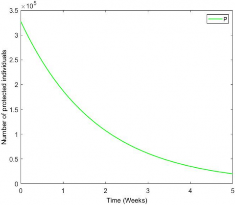
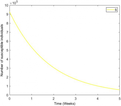
Figure 2. COVID-19 dynamics in classes P, S, I, and T
Figure 3. Comparison of all classes
Figure 2 illustrates a decline in the number of treated patients following infection over time. This phenomenon can be ascribed to the discrepancy between the reported instances of infection and the real number of infections that have transpired but remain unreported. Additionally, the diagram shows the impact of protection measures, specifically vaccination, on mitigating the transmission of the disease in Najaf subsequent to treatment. Furthermore, it has been observed that the population susceptible to the condition decreases as time progresses. The reason for infection is that individuals who are susceptible come into contact, either directly or indirectly, with those who are infected. Following infection, certain individuals may exhibit signs of recovery or succumb to the illness, resulting in a gradual reduction of the infected populace. The administration of vaccinations has been shown to result in a reduction in the rate of infection when compared to individuals who have not received vaccinations.
Furthermore, the findings of the investigation demonstrate a noticeable association between vaccination and the reduction of the transmission of COVID-19. Consequently, precautionary measures are implemented to mitigate the risk of exposure to the virus. To provide a sustainable solution, it is recommended to offer vaccination. The aforementioned factor significantly contributes to the reduction of infection cases in Najaf.
The figures for all cases were collected in Figure 3 for comparison.
In recent times, the COVID-19 pandemic has arisen as a substantial concern within the realm of the general population's health. The PSITPS Model for the COVID-19 epidemic has been. studied. The existence. and uniqueness. of the. solution, as well as its positivity and boundedness have been proven for the proposal Model. The determination of the Basic. Reproduction. Number $\mathcal{R}_0$ is crucial in assessing the potential for disease eradication or spread within a population. The study conducted a stability. analysis, which revealed that the Disease-Free Equilibrium exhibits local asymptotic stability under the condition that $\mathcal{R}_0<1$. Conversely, the Endemic. Equilibrium point is established when $\mathcal{R}_0$ exceeds 1 .
The parameter values for the model were determined through the utilization of actual data obtained from the Public Health Department and the Statistics Division of the Training and Human Development Center of the Najaf Health Directorate. The model studied in this work was run through numerical simulations using the RK4 method in the MATLAB program. The findings of this study suggest that the implementation of protective measures, such as vaccination, significantly contributes to the mitigation of COVID-19 transmission in the region of Najaf for a prolonged duration. Furthermore, it is imperative to implement measures that decrease the contact rate while simultaneously increasing the vaccination rate to effectively manage the disease.
We express our gratitude to thank the Public Health Department and the Statistics Division of the Training and Human Development Center of Najaf Health Directorate\Ministry of Health in Iraq for their cooperation in supporting us with the actual data of COVID-19 infected cases (NO.47856\Date: 2022\11\23 and NO.49146\Date: 2022\11\30, respectively).
[1] Bacaër, N., Bacaër, N. (2011). Daniel Bernoulli, d’Alembert and the inoculation of smallpox (1760). A Short History of Mathematical Population Dynamics, 21-30. https://doi.org/10.1007/978-0-85729-115-8_4
[2] Kermack, W.O., McKendrick, A.G. (1927). A contribution to the mathematical theory of epidemics. In Proceedings of the Royal Society of London. Series A, Containing Papers of a Mathematical and Physical Character, 115(772): 700-721. https://doi.org/10.1098/rspa.1927.0118
[3] Nisar, K.S., Ahmad, S., Ullah, A., Shah, K., Alrabaiah, H., Arfan, M. (2021). Mathematical analysis of SIRD model of COVID-19 with Caputo fractional derivative based on real data. Results in Physics, 21: 103772. https://doi.org/10.1016/j.rinp.2020.103772
[4] Annas, S., Pratama, M.I., Rifandi, M., Sanusi, W., Side, S. (2020). Stability analysis and numerical simulation of SEIR model for pandemic COVID-19 spread in Indonesia. Chaos, Solitons & Fractals, 139, 110072. https://doi.org/10.1016/j.chaos.2020.110072
[5] Viguerie, A., Lorenzo, G., Auricchio, F., Baroli, D., Hughes, T.J., Patton, A., Reali, A., Yankeelov, T.E., Veneziani, A. (2021). Simulating the spread of COVID-19 via a spatially-resolved susceptible-exposed-infected-recovered-deceased (SEIRD) model with heterogeneous diffusion. Applied Mathematics Letters, 111: 106617. https://doi.org/10.1016/j.aml.2020.106617
[6] Zhong, N.S., Zheng, B.J., Li, Y.M., Poon, L.L.M., Xie, Z.H., Chan, K.H., Li, P. Tan, S., Chang, Q., Xie, J., Liu, X., Xu, J., Li, D., Yuen, K., Peiris, J., Guan, Y. (2003). Epidemiology and cause of severe acute respiratory syndrome (SARS) in Guangdong. People's Republic of China. The Lancet, 362(9393): 1353-1358. https://doi.org/10.1016/S0140-6736(03)14630-2
[7] Wang, N., Shi, X., Jiang, L., Zhang, S., Wang, D., Tong, P., Guo, D., Fu, L., Cui, Y., Liu, X., Arledge, K.C., Chen, Y.H., Zhang L., Wang, X. (2013). Structure of MERS-CoV spike receptor-binding domain complexed with human receptor DPP4. Cell Research, 23(8): 986-993. https://doi.org/10.1038/cr.2013.92
[8] Lai, C.C., Shih, T.P., Ko, W.C., Tang, H.J., Hsueh, P.R. (2020). Severe acute respiratory syndrome coronavirus 2 (SARS-CoV-2) and coronavirus disease-2019 (COVID-19): The epidemic and the challenges. International Journal of Antimicrobial Agents, 55(3): 105924. https://doi.org/10.1016/j.ijantimicag.2020.105924
[9] Du Toit, A. (2020). Outbreak of a novel coronavirus. Nature Reviews Microbiology, 18(3): 123-123. https://doi.org/10.1038/s41579-020-0332-0
[10] World Health Organization. (2020). Coronavirus disease 2019 (COVID-19): Situation report, 99. https://apps.who.int/iris/handle/10665/331909.
[11] Government of Iraq. (2020). Novel coronavirus (COVID-19): Iraq’s ministry of health guidance to the public Web log post. https://gds.gov.iq/novel-coronavirus%e2%80%aacovid-19-iraqs-ministry-of-health-guidance-to-the-public/, accessed on Nov. 28, 2023.
[12] Government of Iraq. (2020). Novel coronavirus (COVID-19): Update from Iraq’s ministry of health Web log post. https://gds.gov.iq/novel-coronavirus/, accessed on Nov. 28, 2023.
[13] World Health Organization, https://covid19.who.int/region/emro/country/iq, accessed on Nov. 28, 2023.
[14] Al-Najaf Health Directorate, “epidemiological situation”, The epidemiological situation of Najaf Health Department, accessed on Nov. 28, 2023. https://alnajafhealth.gov.iq/archives/155191, accessed on Nov. 28, 2023.
[15] Ministry of Health, Al-Najaf Al-Ashraf Governorate, Najaf Health Directorate, Training and Human Development Center, Public Health Department, No. 47856. https://alnajafhealth.gov.iq/.
[16] Abidemi, A., Zainuddin, Z.M., Aziz, N.A.B. (2021). Impact of control interventions on COVID-19 population dynamics in Malaysia: A mathematical study. The European Physical Journal Plus, 136: 1-35. https://doi.org/10.1140/epjp/s13360-021-01205-5
[17] Lobato, F.S., Libotte, G.B., Platt, G.M. (2021). Mathematical modelling of the second wave of COVID-19 infections using deterministic and stochastic SIDR models. Nonlinear Dynamics, 106(2): 1359-1373. https://doi.org/10.1007/s11071-021-06680-0
[18] Rida, S.Z., Farghaly, A.A., Hussien, F. (2021). Global dynamics and sensitivity analysis of seiar mathematical model for COVID-19 pandemic. Assiut University Journal of Multidisciplinary Scientific Research, 50(2): 1-18. https://doi.org/10.21608/aunj.2021.219661
[19] Mustafa, A.N., Ahmad, H.J. (2022). Modeling the effect of contaminated object, vaccination and treatment on the diseases epidemiology. Passer Journal of Basic and Applied Sciences, 4(2): 105-112. https://doi.org/10.24271/psr.2022.330125.1119
[20] Hamou, A.A., Rasul, R.R., Hammouch, Z., Özdemir, N. (2022). Analysis and dynamics of a mathematical model to predict unreported cases of COVID-19 epidemic in Morocco. Computational and Applied Mathematics, 41(6): 289. https://doi.org/10.1007/s40314-022-01990-4
[21] Salam, B.A., Khoshnaw, S.H., Adarbar, A.M., Sharifi, H.M., Mohammed, A.S. (2022). Model predictions and data fitting can effectively work in spreading COVID-19 pandemic. AIMS Bioeng, 9: 197-212. https://doi.org/10.3934/bioeng.2022014
[22] Rai, S. (2022). Dynamical study of Covid-19 in Nepal with vaccination. Doctoral Dissertation, Kathmandu University.
[23] Mohammed, A.S., Khoshnaw, S.H. (2023). The impact of vaccination on COVID-19 pandemic in the Kurdistan Region of Iraq: A mathematical modelling. Palestine Journal of Mathematics, 12: 87-106.
[24] Satar, H.A., Naji, R.K. (2023). A mathematical study for the transmission of coronavirus disease. Mathematics, 11(10): 2330. https://doi.org/10.3390/math11102330
[25] Wameko, M.S., Wedajo, A.G., Koya, P.R. (2019). Mathematical model for transmission dynamics of typhoid fever. IOSR Journal of Mathematics (IOSR-JM), 15(6): 88-99. https://doi.org/10.9790/5728-1506028899
[26] Das, K. (2022). Impact of periodicity and stochastic impact on COVID-19 pandemic: A mathematical model. Network Biology, 12(3): 120-132.
[27] Kamgang, J.C., Sallet, G. (2008). Computation of threshold conditions for epidemiological models and global stability of the Disease-Free Equilibrium (DFE). Mathematical Biosciences, 213(1): 1-12. https://doi.org/10.1016/j.mbs.2008.02.005
[28] Tilahun, G.T., Tolasa, T.M., Wole, G.A. (2022). Modeling the dynamics of rubella disease with vertical transmission. Heliyon, 8(11). https://doi.org/10.1016/j.heliyon.2022.e11797
[29] Ministry of Health, Al-Najaf Al-Ashraf Governorate, Najaf Health Directorate, Training and Human Development Center, Statistics Division, No. 49146. https://alnajafhealth.gov.iq.