Zahraa Ch. Oleiwi![]() | Ebtesam N. AlShemmary*
| Ebtesam N. AlShemmary*![]() | Salam Al-Augby
| Salam Al-Augby![]()
© 2024 The authors. This article is published by IIETA and is licensed under the CC BY 4.0 license (http://creativecommons.org/licenses/by/4.0/).
OPEN ACCESS
There are many methods to diagnose heart disease; the most effective way is to analyze electrocardiogram (ECG) signals. Generally, the automatic classification techniques based on ECG analysis consist of three steps: data preprocessing, feature extraction, and classification. This study designed eight hybrid model architectures using several types of deep neural networks, including Convolution Neural Network (CNN), Gated Recurrent Unit (GRU), and Bidirectional GRU (Bi-GRU), four of them without Fast Fourier Transform (FFT) and the rest using FFT. Firstly, the MIT-BIH arrhythmia database is cleaned using the wavelet (WT) thresholding method that separates the combined noise and signal frequencies, making it ideal for processing nonstationary ECG signals. Additionally, the imbalance problem in this database was addressed using the synthetic minority over-sampling technique (SMOTE), which is more suitable for medical data than random synthesis methods. Secondly, hybrid models FFT-CNN, FFT-GRU, FFT-CNN-GRU, and FFT-CNN-Bi-GRU are constructed using the new proposed architecture by concatenating resultant features from two paths, the first path using ECG in the time domain and the second path using the resultant spectrum of ECG from FFT as input. A comparative study of the performance of all models was created in terms of accuracy, training time, number of trainable parameters, and robustness against noise. The results show that the proposed CNN, GRU, CNN-GRU, and CNN-Bi-GRU models without WT and FFT achieved 90%, 93%, 95%, and 96% accuracies, while the proposed FFT-CNN, FFT-GRU, FFT-CNN-GRU, and FFT-CNN-Bi-GRU models achieved 97%, 95%, 96%, and 97% accuracies with WT. So, the proposed FFT-CNN model was the best, with less training time and parameters than other models, which significantly impacts designing a high-efficiency model with less complexity for a practical medical diagnosis system. On the other hand, using FFT improved all models' performance, accuracy and robustness against noise.
deep learning, arrhythmia prediction, heart disease diagnosis, Bi-GRU, Convolution Neural Network, electrocardiogram, Fast Fourier Transform based feature extraction, Gated Recurrent Unit
Heart disease (i.e., coronary artery disease, arrhythmias) is a severe disease. Early detection is crucial in effectively managing these diseases and reducing the risk of fatal consequences [1]. The problem of heart rhythm is called arrhythmias which refers to an irregular and abnormal heartbeat [2]. There is more than one primary type of arrhythmias: atrial fibrillation (AF), where the heartbeat is faster than normal; supraventricular tachycardia, where the heartbeat is more rapid than normal at rest; bradycardia, where the heartbeat is slower than usual; heart block where the heartbeat is slower than expected which led to collapse, and ventricular fibrillation where the heartbeat is rapid and disorganized which may cause the patient to lose his consciousness or sudden death [3].
All these dangerous types can be treated, and the patient can be saved from them if detected early. In light of the preceding, automated techniques play an important role in detecting these diseases automatically, quickly, efficiently, and adequately. For example, early detection and appropriate treatment of Atrial Fibrillation can reduce the risk of stroke and lead to a near-normal life expectancy [4].
The analysis of ECG signals is essential to detect arrhythmias, so many researchers use ECG datasets to design arrhythmias classification and prediction models based on machine and deep learning algorithms [5, 6].
ECG signals provide features like QRS complex, RR interval, and waveform similarity for machine learning models. Time and frequency domain features, along with statistical and morphology features, are used. Common algorithms include support vector machine, random forest, decision tree, k-nearest neighbor, Bayesian algorithm, and artificial neural network [7, 8].
The challenge in using the mentioned above machine learning is feature extraction. This process requires time and experience, as any error in this step will diverge in all subsequent actions within the model, ultimately impacting its performance [9]. As a result, the other research category depends on a deep learning model with no feature extraction step [10].
CNN alleviated the obstacle of manual feature extraction. So many classification models were constructed based on CNN, which achieved good results [11].
Recurrent Neural Networks (RNN), Long Short-Term Memory (LSTM), GRU, and BiGRU are well-known deep learning architectures that manipulate time series signals. Hybrid models for the Arrhythmias classification were constructed based on these architectures and CNN [12].
Most of the research that used CNN and other deep learning techniques did not use Fourier transform (FT) to extract the features of the frequency domain based on CNN. So, in this work, four hybrid models based on FFT and CNN are designed using ANN, GRU, and Bi-GRU, with a comparative study to identify the best model. The key contributions of the paper are summarized as follows:
•Features from the frequency domain of ECG signals are extracted and concatenated with extracted time domain features using the proposed CNN architecture. This network constructed from two parallel stages of convolution layers, one step for the original ECG signals (to extract time domain features) and a second stage for FFT spectrum of the original ECG signals (to extract frequency domain features).
•A novel eight ECG classification hybrid model architectures of deep neural networks (CNN, GRU, Bi-GRU) for arrhythmia prediction are proposed. Four including FFT and the rest not, with the aim of extract deeper and more relevant and discriminatory features to improve the performance of CNN.
•The effectiveness of using FFT on the performance of proposed CNN-based models is demonstrated by analyzing a comparative study for all proposed models in terms of four evaluation metrics.
•Producing a comparative study of how a denoising method affects the performance of CNN models and highlights their robustness against noise. This study includes an analysis of the models' performance with and without the method.
The rest of this paper is organized as follows. First, the related work is described in Section 2. Section 3 explains the materials and methods used in this paper. Section 4 defines and describes the proposed models. Section 5 discusses the results and analysis of the proposed techniques. Finally, the conclusions are presented in Section 6.
The most crucial information on signals is concentrated in the frequency domain, and this information is essential for accurate decisions the classification algorithms need to achieve high classification accuracy [13, 14].
The objective of hybridization is to improve classification evaluation results' performance by increasing the dimensionality of data and extracting more discriminatory features for designing classification models. This improvement was achieved for hybrid models trained on different datasets, not only the ECG dataset, where in literature [15] a hybrid deep learning model constructed from a convolutional neural network (CNN) and a long short-term memory (LSTM) layer for speech emotion recognition was proposed. The result of the evaluation of this work on four different speech datasets in terms of recognition accuracy was about 99% which proved the superiority of this work as compared with state-of-the-art models.
Multiple classification models are constructed using a different version of recurrent neural network (RNN) combined with CNN as feature extraction. These versions include RNN, LSTM, and GRU, with additional layers in each model. For 1000 epochs, the five-fold cross-validation accuracy was 83,7% achieved using a hybrid model with three layers of CNN and GRU, considered the best among the multiple models designed in this work [16].
Another work that combined CNN with the GRU in different architectures was produced in literature [17] to classify five types of heartbeat. This model was designed using one convolution layer and six local feature extraction modules (LFEM), then the resultant features passed to GRU, then to the Dense layer, and finally using the SoftMax layer as decision-making to classify five types of heart rhythms. This model achieved a classification accuracy of about 99%.
A new technique in combining two different deep learning algorithms to extract important features was developed in literature [18], where dilated CNN and two versions of Bidirectional RNN bidirectional Gated Recurrent Units (Bi-GRU) and bidirectional long short-term memory (Bi-LSTM) were combined. The resultant features from Bi-GRU and Bi-LSTM were concatenated and then passed to CNN for connection. This hybrid architecture improved the performance of dilated CNN and increased the classification accuracy to 99.9%.
As we mentioned before, the features extracted from the frequency domain increase the discriminatory representation of the data since the frequency domain rich with more relevant features will improve the performance of the classification modes; this was confirmed in literature [19], where the proposed classification deep learning model based on time-frequency representations (TFRs) of noisy non-stationary signals. In this work, the deep learning models were constructed using the most common CNN architectures: ResNet-101, EfficientNet, and Xception. The results achieved by these TFRs-based deep CCN models show significant performance improvement as compared with models trained with originals signals without using TFRs, where the classification results were evaluated by different metrics such as accuracy, recall, and precision which were about 97%, 95%, and 99 respectively. These metrics values were higher than those obtained using the base model with original data.
Two dimensions-CNN was used to classify five types of heartbeat for the 1D time domain of ECG signal by converting it to a 2D time-frequency spectrum using a short-time Fourier transform. This technique achieved a high accuracy of about 99% compared to the accuracy achieved in the case of using 1D-CNN, which gained 90% classification accuracy [20].
Fourier transform plays an essential role in the performance improvement of 2D-CNN by concatenating the QRS complex in the time domain with the resultant spectrum of FFT of the signal to construct 2D input. The 2D concatenation input enters CNN's three convolution layers. This model raises the accuracy of classification to 99% [21].
According to our understanding and what we have read from the above studies, the ID frequency spectrum was not utilized as input to 1D-CNN to extract frequency domain features and then concatenate them with time domain features using several deep learning approaches, as was done in this study. Compared to prior works, this study saves time and complexity by developing CNN architecture with fewer structural complexities, the number of layers, and trainable parameters.
A comparison of the methods used in these studies including the proposed work in this paper are illustrated in Table 1.
Table 1. The summary table of related previous works compared with the proposed work
|
Ref. |
Type of Feature Domain |
Model Architecture |
#Epochs |
#Classes |
|
[16] |
1-D data input of Time domain signal |
1-D CNN 3 layer with GRU 1 layer and 64 unit and fully conected network |
1000 |
2 |
|
[17] |
1-D data input of Time domain signal |
Convolution layer, followed by 6 LFEM, a GRU, and a Dense layer and a Softmax layer |
200 |
5 |
|
[18] |
1-D data input of Time domain signal |
Bidirectional RNN with multilayer Dilated CNN (BRDC), fully connected layer and Rectified Linear Unit (ReLU) |
100 |
5 |
|
[21] |
2-D data input from Combination of the FFT-based frequency and the RR interval features |
2-D CNN 3 convolution layers with 2 batch normalization and pooling layers follow by 2 fully connected layers |
- |
5 |
|
[20] |
2-D time-frequency spectrograms of ECG segment |
2D-CNN with 3 convolution and 3 pooling layers follow by shallow neural network |
100 |
5 |
|
Proposed model |
Seperated 1-D data input of Time domain signal and 1-D data input of FFT- based frequency domain signal |
Two path of 1-D CNN 3 covolution and 3 pooling layers following by flatten and softmax layer |
7 |
5 |
As is clear from Table 1, the works in literatures [15-17] used only time domain features with a more complex network and a greater number of epochs. In contrast, the work in [20, 21] increased its complexity by using 2-D data input using frequency domain features with a high complexity network and more epochs. So, the proposed work overcame these complexities by using time and frequency features as 1-D input data with simple network architecture and seven epochs only.
This section explains all the methods and descriptions related to database and processing database and the method used for constructing classifier network.
3.1 Database description
The standard MIT/BIH arrhythmia database was used to implement this study. This database contains 48 out of 30 minutes of two-channel ECG records for 47 patients. The sampling frequency of the ECG recordings was digitalized with 360 HZ and 11 bits resolution over a 10 Mv range. This database is available at (https://physionet.org/content/mitdb/1.0.0/). The total number of samples that represent the number of sampled beats was 109446, with five categories [22]:
['N': 0, 'S': 1, 'V': 2, 'F': 3, 'Q': 4]
where,
N: Non-Ectopic beats (normal beat),
S: Supraventricular ectopic beats,
V: Ventricular ectopic beats,
F: Fusion Beats, and
Q: Unknown Beats.
These signals are preprocessed and segmented, with each segment corresponding to the heartbeat.
3.2 Data preprocessing
ECG signals were corrupted by different types of noise, such as Electromyography (EMG) interference, power frequency interference, and baseline drift, which affect classification accuracy. Therefore, the researchers first removed the noise using different method [23].
Discrete Wavelet Transform (DWT) in literature [24] filters ECG signals from high-frequency noise, power line interference, and baseline wander. Important signal information can be obtained from wavelet transform [25]. The first set of coefficients is called Approximation Coefficients, which are low-frequency coefficients (containing the essential information of the signal), and the second set is called Details Coefficients, which are high-frequency coefficients (small values coefficients as compared with Approximation Coefficients which have large values) [26]. Since the noise is characterized by high band frequency, it focuses on high-frequency Details Coefficients. As a result of these phenomena, wavelet transform can be used as a noise removal filter by thresholding the coefficients with appropriate threshold values [27]. There are multiple thresholding functions, such as hard and soft functions. The work-hard threshold function is used as follows [28]:
$y(x)= \begin{cases}x & |x|>\gamma \\ 0 & |x| \leq \gamma\end{cases}$ (1)
where, $\gamma$ is the threshold value selected according to the universal threshold (VisuShrink) known for its simplicity and effectiveness. The formula is denoted as:
$\gamma=\sigma \sqrt{2 \ln (N)}$ (2)
where, N is the length of the signal, and $\sigma$ is the average variance of the noise, which is computed as follows:
$\sigma=\frac{\text { medium }\left|W_{1, k}\right|}{0.6745}$ (3)
The wavelet family uses symlets. $W_{1, k}$ is all wavelet coefficients in scale one [28].
An imbalanced database means that the number of examples in each class is unequally distributed [29]. This work deals with the MIT imbalanced database where the number of samples belonging to a normal class is more than the number of samples in all reset classes.
This problem caused the degradation of the classification model performance in terms of accuracy due to the biased results toward the majority class and ignoring the minority class due to considering it as noise data [30]. On the other hand, many machine learning algorithms are designed with the assumption that the database is balanced [31]. There are many solutions to this problem; one is under-sampling, where the number of samples is selected from a normal class (majority class) approximately equal to the number of samples in other classes (minority classes), for example, 10000 samples. This solution will reduce the total number of samples in the dataset (reduce the size of the database), and this will cause another problem, such as underfitting, as well as some of the information needing [32].
On the other hand, oversampling generates more samples for minority classes by replicating the examples in these classes and solves the imbalance problem, but it causes an overfitting problem [33].
Another solution is to consider the problem as a binary classification and solve the problem as follows:
1-Collect samples of all abnormal classes in one class.
2-Perform the binary classification as the first stage of classification of normal vs abnormal.
3-Enter the abnormal test sample into the second classification stage to classify it into corresponding irregular classes from four types of abnormal classes.
This solution takes more time and complexity, so this work went toward the best solution, the SMOTE-based augmentation method, without repeating samples [34].
The augmentation technique increases the size of the database by generating more samples using processing techniques such as scaling, rotation, cropping, flipping, etc. This processing technique is suitable for images, but it is not appropriate for ECG signals since it changes the morphology of the signal and then it loses original information [35].
This work used the Synthetic Minority Oversampling Technique (SMOTE) as it is explained as follows:
1-Under-sampling the majority of the class (normal class) from 70000 to 20000 samples.
2-Passing minority classes to SMOTE function, which works as:
-Determining the K-nearest neighbour for each $X_i$ sample in each minority class using Euclidian distance.
-Determining the sampling ratio for each class, i.e., N.
-For each $X_i$ determine N random numbers from their nearest neighbor, and for each $X_n$ generate a new sample according to Eq. (4) [6]:
$X_{N E W}=X_n+\mu\left(X_i-X_n\right)$ (4)
where, μ is a small random factor in the range of (0,1).
-Repeat this Eq. (4) until generating N corresponding to each $X_i$. If the total size of the minority class is M then the new size is NM.
In this work, the NM=20000 samples for each minority class. Therefore, the entire training set increased from 87553 to 100000 examples.
3.3 FFT
The signal's frequency content can be revealed using one of the most common transforms called the FT [35]. This frequency content is called spectrum and is expressed as [27]:
$X(f)=\int_{-\infty}^{\infty} x(t) e^{-j 2 \pi f t} d t$ (5)
$x(t)=F^{-1}\{X(f)\}=\int_{-\infty}^{\infty} X(f) e^{+j 2 \pi f t} d f$ (6)
The X(f) spectrum is represented by the magnitude spectrum denoted by $|X(f)|$ and the phase spectrum indicated by $\angle X(f)$. Fast Fourier Transform (FFT) is the efficient algorithm used to compute Fourier transform, which was proposed in 1965 [36].
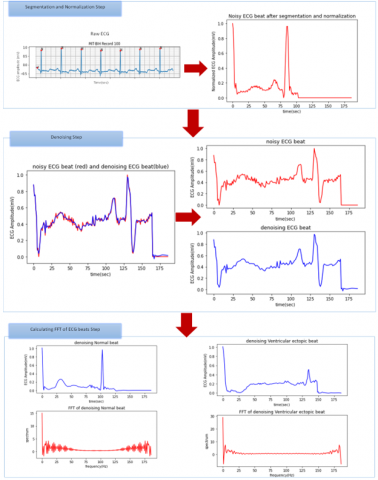
The motivation beyond the analysis of the signal in the frequency domain is that the essential characteristics and information of the signal can be revealed from the frequency domain. In addition, the frequency domain provides valuable tools to analyze the signal. However, the frequency domain will produce a better rich environment with features that classify the signal [27, 37]. All the preprocessing steps and calculating the FFT of ECG beats are illustrated and shown in Figure 1.
3.4 CNN as feature engineering
Convolutional neural networks consider a class of ANN that simulate the operation of the human brain's visual cortex and are used for feature engineering instead of manual feature extraction. The CNN handles the signal directly by applying a filter to it to produce the number of feature maps equal to the number of filters (array of weights called the kernel) [38, 39]. The mechanism of the works of CNN can be illustrated below steps:
1-An input layer represents the direct data of a signal or image.
2-Convolution layer: In this layer, the convolution operation applies input using several filters to produce feature maps.
3-Applying rectified linear activation function (ReLU) activation function on resultant feature maps to process them as in an ordinary deep neural network.
4-Reduce the dimensions of feature maps using the mean or max operation in the MaxPooling layer. The benefit of this layer is reducing the computational load as well as reducing overfitting.
5-Converting the results from 2D to 1D Flatten vector that passes to the artificial neural network, which works as the classifier. Usually, this fully connected network (ANN) consists of three layers, input layers, a hidden layer, and an output layer. Figure 2 explains the main architecture of CNN.
Through experimentation, it has been discovered that the selection of filters, their sizes, and their quantity can greatly impact the performance of a CNN. Typically, the upper convolution layer utilizes larger filter sizes, while subsequent layers use smaller filter sizes and increased numbers of filters. It has been observed that the accuracy of the results is negatively affected by larger filter sizes and positively impacted by a higher number of filters [40].
It is typical for a larger filter to lose important patterns and detailed information compared to a smaller filter. The filter's small size allows for capturing the most important information and patterns, especially those with rapid changes. This is particularly true for the ECG signal, characterized by short oscillation intervals. Therefore, a small-sized filter was chosen for this work to match the nature of the signal, which is (1*3) [41].
3.5 GRU and BIGRU
RNN is a neural network designed to feed back the output of one layer to the input for layer output prediction [42, 43].
Figure 1. The preprocessing and FFT steps of ECG beats signals
Figure 2. The main architecture of CNN
RNN handles sequential data (time series) so that the input x at any given time (t) is denoted by xt combined with the input from the previous time xt-1. So the output at any given time depends on current and previous input data [44].
Although the RNN plays a good role in solving time series problems such as time series prediction and in natural language processing, it has several drawbacks; one of them is the vanishing problem, where the updating of deeper parameters became inaccurate when the gradient was too small. Another problem is that the RNN handles only short-term dependencies [42, 45].
To address the issue of long-term dependencies, a superior version of RNN known as LSTM was developed. The idea of the LSTM based on it is to use three gates: input gate, forget gate, and output gate
The first step in LSTM is implementing in forget gate to determine the unimportant information from the previous time step and delete it. The function of the forget gate is [42, 46]:
$f(t)=\sigma\left(W_f \cdot\left[h_{t-1}, x_t\right]+b_f\right)$ (7)
The second step is implementing an input gate to determine the important information and let it pass from the previous time step to the current action. The function of the input gate is [19]:
$i(t)=\sigma\left(W_i \cdot\left[h_{t-1}, x_t\right]+b_i\right)$ (8)
$C_t=\tanh \left(W_c \cdot\left[h_{t-1}, x_t\right]+b_c\right)$ (9)
The third step is implementing an output gate to impact the output of the current time step by significantly passing information. The function of the output gate is [19]:
$O(t)=\sigma\left(W_o \cdot\left[h_{t-1}, x_t\right]+b_o\right)$ (10)
$h_t=o(t) * \tanh \left(C_t\right)$ (11)
A simplified version of LSTM is known as Gated Recurrent Units (GRUs) which is a gating mechanism based on RNN, considered an enhanced version of LSTM. In contrast to LSTM, GRU consists of only two gates: the update gate and reset gate, instead of three gates as in LSTM. So, it has fewer parameters easier to implement than LSTM [47].
When comparing LSTM and GRU, the key differences lie in their architecture and trade-offs. LSTM is more flexible and expressive than GRU but more computationally costly and prone to overfitting. In contrast, GRU has fewer gates and parameters, making it faster, simpler, and less powerful. Additionally, LSTM can store and output different information since it has a separate cell state and output. Whereas GRU has a single hidden state for both functions, which may limit its capacity. It's important to note that LSTM and GRU may have varying sensitivities to hyperparameters like learning rate, dropout rate, and sequence length.
When it comes to natural language processing tasks like sentiment analysis, machine translation and text generation, the performance of LSTM and GRU can depend on various factors such as the task, data and hyperparameters. Empirical studies have shown that these two models perform similarly in many cases. However, there are some tasks where one of them might be more beneficial than the other. For instance, tasks like speech recognition, image captioning or video analysis may benefit from the unique features of either LSTM or GRU.
GRU is similar to LSTM in using a gate mechanism for information flow control, but it has a more straightforward structure than LSTM. Each time step takes only input xt and hidden state ht-1) from the previous step and passes ht as output for the next step (GRU unit) [12, 48].
The essential characteristic of the gates of GRU is keeping the information for a long ago without forgetting it over time as well as it doesn't remove irrelevant information with prediction. So, it can solve vanishing problems with better and more efficient performance than LSTM [49].
GRU works according to the following steps:
1-Short-term memory is the Reset gate's responsibility, represented by a hidden state ht. The function of the Reset gate is [50]:
$r_t=\sigma\left(x_t * U_r+h_{t-1} * W_r\right)$ (12)
2-Generating the candidate's hidden state as [50]:
$\hat{h}_t=\tanh \left(x_t * U_g+\left(r_t{ }^{\circ} h_{t-1}\right) * W_g\right)$ (13)
The essential part of the Eq. (13) is rt which determines the value of the Reset gate, which is used to control how much the previously hidden state had an impact on the candidate's hidden state, that is:
If rt=1, all information from the previous state ht-1 will be considered.
If rt=0 then all information from the previous state ht-1 will be ignored.
3-Long-term memory is the responsibility of the update gate. The function of the update gate is [50]:
$u_t=\sigma\left(x_t * U_u+h_{t-1} * W_u\right)$ (14)
4-Generating the currently hidden state ht as [50]:
$h_t=u_t h_{t-1}+\left(1-u_t\right) \hat{h}_t$ (15)
An essential part of the above equation is the value of the update gate ut, which controls both information from the candidate's state $\hat{h}_t$ and the historical information ht-1 as follows:
If ut=0, then ut ht-1 will vanish, so the information from the previous state ht-1 is ignored, and the information from the candidate's state $\hat{h}_t$ is considered, and vice versa if ut=1.
Clearly, the GRU has only one hidden state to capture past information. To overcome this limitation, the enhancement version of GRU was developed, known as Bidirectional GRU (Bi-GRU), with the idea of constructing two neural networks.
A Bi-GRU has two hidden states, one for each direction. A forward neural network and a backward neural network allow past and future information to impact the current state. Finally, the output layer connects the two outputs from the two networks [12, 51]:
In the forward layer, the output of the hidden layer is calculated each time from forward to backward. While in the backward layer, the output of hidden layers is calculated in opposite directions from backward toward forward. In the output layer, the two outputs resultant from the two layers are normalized and composed each time.
The functionality equations of forwarding and backward network layers in Bi-GRU are expressed as [51, 52]:
$\overrightarrow{h_t}=G R U_{f w d}\left(x_t, \overrightarrow{h_{t-1}}\right)$ (16)
$\overleftarrow{h_t}=G R U_{f w d}\left(x_t, \overleftarrow{h_{t+1}}\right)$ (17)
$y_t=\overrightarrow{h_t} \oplus \stackrel{\leftarrow}{h_t}$ (18)
where,
$\overrightarrow{h_t}$ is the output of forward hidden states, the forward layer in Bi-GRU is calculated.
$\overleftarrow{h_t}$ is the output of backward hidden states, the backward layer in Bi-GRU has calculated it.
The $\oplus$ symbol refers to concatenating between $\overrightarrow{h_t}$ and $\overleftarrow{h_t}$, done in the output layer.
In practice applications, Bi-GRUs are commonly utilized for tasks such as natural language processing. This is because the model needs to comprehend the context of a word in a sentence to provide precise predictions.
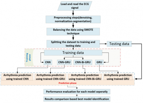
This work includes two stages: the first stage is based on the time domain feature to construct four classification models, as in the below steps:
1-The raw beat segment of ECG is entered into CNN as a feature extraction technique which is constructed from three convolution layers and three MaxPooling layers of size (2*1). The top convolution layer has 16 filters, the second layer has 32 filters, and the third layer has 64 filters. Each filter has a size of (3*1).
2-The Flatten vector resultant from the first step is entered into ANN of single layer as a multiclass classifier with five classes of arrhythmias using the SoftMax activation function.
3-Repeat steps 1 and 2 to create two separate hybrid models, namely CNN-GRU and CNN-Bi-GRU, use a single layer of GRU and BI-GRU with 128 and 256 units respectively instead of using flatten layer. Final layer in these models is SoftMax layer with 5 units.
4-For the fourth model, the raw beat segment of ECG is inputted directly to three layers of GRU without using CNN. The top layer has 32 units, followed by 64 units in the second layer, and 128 units in the third layer. The final layer is SoftMax with 5 units.
For this study, the GRU was selected to tackle complexity and overfitting concerns as it is known for this ability. The objective is to develop a more efficient model for short ECG segments without having to capture long-term dependencies.
As previously mentioned, Bi-GRUs are often used in natural language processing tasks. This is due to the model's ability to understand the context of a word in a sentence, which results in accurate predictions. This feature is also beneficial for ECG, which is why the proposed work utilizes this model. The Bi-GRU combines the advantages of both GRU and LSTM.
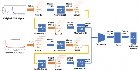
In the second stage of our proposed work, four hybrid models based on FFT of raw ECG and beat segments are constructed. The architecture design for the proposed models is illustrated in the below steps.
1-Inputting the original signal x(t) as a first path to the first CNN (with the same architecture of CNN in the first stage) to extract time domain features as a vector of time domain features.
2-Transforming ECG beat segment x(t) to the frequency domain using FFT to obtain X(f).
3-Inputting the resultant signal X(f) as a second path to the second CNN (with the same architecture of CNN in first stage) to extract frequency domain features as vector of frequency domain features.
4-Concatenating the resultant two vectors from steps 1 and 3 to obtain the final hybrid vector of time and frequency domain features and then construct flatten vector via flatten layer.
5-Inputting the final hybrid Flatten vector to single SoftMax layer of five units as a multiclassification classifier.
6-The sixth model comprises of two paths, with each path having two GRU layers consisting of 32 and 64 units, respectively. The original time domain signal x(t) enters the first path, and the frequency domain signal X(f) enters the second path. The resulting feature vector is then combined and enters the third GRU layer with 128 units. Then the SoftMax layer is used with 5 units as a multiclass classifier.
7-To create two distinct hybrid models, namely FFT-CNN-GRU and FFT-CNN-Bi-GRU, repeat steps 1to 5. Instead of using a flatten layer, utilize a single layer of GRU and BI-GRU with 128 and 256 units, respectively.
In order to classify the various types of ECG samples that have high overlap and correlation, CNN was utilized to extract deeper features that can act as discriminators. To achieve this, frequency features that based on FFT were extracted using CNN. The signal frequencies' spectra offer distinct and precise data with more details from the frequency domain that can serve as a foundation for decision-making.
The final step of the two stages is comparing the above models' results to identify the best method for accuracy, recall, precision, F1-score, and the number of parameters in each architecture. In addition, statistical analysis across different runs based on mean, standard deviation, and Friedman test was used. This statistical analysis helps for multiple model comparison.
When there is a significant imbalance between classes, such as in Arrhythmia detection using ECG heartbeat classification, it is important to consider the recall (sensitivity) metric as it is the most reliable in medical diagnosis. Recall refers to the number of correctly classified samples, and is particularly important for the abnormal ECG class. This is because it reflects how well the models are able to detect abnormalities. When the recall is low, this means that abnormalities may go undetected, leading to delayed diagnosis and even death.
Figure 3 and Figure 4 illustrate the general proposed framework for constructing hybrid models.
Figure 3. General framework for the first stage of the proposed work
Figure 4. General framework for the second stage of the proposed work
The dataset is divided randomly into a training dataset and a testing dataset, with a ratio of 8:2. The training set is used to train the classification model in the proposed model, while the testing set is used to evaluate the performance of the model's classification effect.
The models are trained using 7 epochs, Adam optimizer, learning rate is 0.001, and the categorical cross entropy loss function.
During model training, the loss function compares predicted results to actual data to determine accuracy. A smaller loss function during training indicates a more precise model classification. In this work, the Categorical-Cross-entropy function is used as the cost function to overcome the traditional loss function's slow parameter updates. The Adam optimizer, proposed by Kingma and Leiba in 2014, is a stochastic gradient descent method that calculates update step size based on adaptive estimation of first-order and second-order moments is used in this project since it combines the benefits of Adagrad and Rmsprop. The Adam optimizer can automatically adjust the learning rate with minimal computation, making it well-suited to datasets with large samples.
5.1 Performance results of CNN model without using SMOTE technique
Without using the augmentation technique, the result of the overfitting problem appeared clearly due to an imbalanced dataset. Figure 5 shows the classification results for the CNN-ANN model. The degradation in the model's generalization performance, caused by overfitting, appears despite using 50 epochs.
Figure 5. CNN Training results without augmentation SMOTE method
Not all datasets, especially medical data, can be augmented using augmentation techniques based on reddening samples, flipping, rotation, etc., of operations since this operation has led to the loss of important information. On the other hand, augmentation methods based on repeated samples will solve the imbalance dataset problem, but it causes overfitting.
Figure 6. The architecture of the first CNN-ANN model
Figure 7. The architecture of the second GRU Mode
Figure 8. The architecture of the third CNN-GRU Model
Figure 9. The architecture of the fourth CNN-Bi-GRU model
Figure 10. Validation results in terms of accuracy without using thresholding denoising method for (A) CNN-ANN model, (B) GRU model, (C) CNN-GRU model, (D) CNN-Bi-GRU model
5.2 Performance results of hybrid models without FFT
The four proposed models were designed to manipulate the dataset and use it to classify five types of arrhythmias without using FFT to extract frequency domain features. The architectures of the four models are shown in Figures 6-9.
All the above four models were trained and tested with and without the denoising process to evaluate the robustness of the models against the noise. Figure 10 shows the training process results for the four models (without wavelet threshold denoising process) in terms of training accuracy and validation accuracy.
As is clear from the above figures, the Bi-GRU is the most robust model against noise than other models where it has the highest accuracy.
Figure 11. Validation results in terms of accuracy by using thresholding denoising method for (A) CNN-ANN model, (B) GRU model, (C) CNN-GRU model, (D) CNN-Bi-GRU model
In terms of training time, the GRU model spent the highest amount of time on training and required more trainable parameters than other models. In contrast, the vanilla CNN needed less time and parameters for training. For this reason, we focus on enhancing the first model's performance in terms of accuracy to obtain an efficient model. Figure 11 shows the training process results for the four models (with the denoising process) in terms of training accuracy and validation accuracy. The thresholding wavelet method was our first attempt to improve the first model (CNN-ANN).
The results in the above figures show that the performance of the first model, CNN-ANN, was improved, and the accuracy was raised with a clear impact of the thresholding method. In contrast, the third CNN-GRU model and the fourth CNN-Bi-GRU model had an effect. This thresholding method did not affect the performance of the second GRU model since the accuracy was fixed at 93% in both cases.
Figure 12. The architecture of the fifth hybrid FFT-CNN-ANN model
Figure 13. The architecture of the sixth hybrid FFT-GRU model
5.3 Performance results of hybrid models with FFT
The second attempt to improve the first CNN model is to use FFT as the first step in the design of the model, where the signal is transformed into the frequency domain, and the resultant 1D spectrum is entered into CNN. All details of the proposed architecture are illustrated in Figures 12-15.
Thresholding method. In contrast, the third CNN-GRU model and the fourth CNN-Bi-GRU model had an impact. This thresholding method did not affect the performance of the second GRU model since the accuracy was fixed at 93% in both cases.
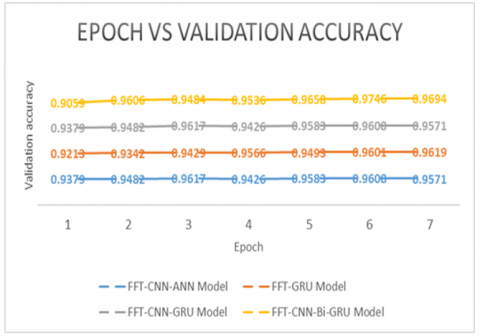
As it is clear from the above figures, the fifth, sixth, seventh, and eighth models were constructed from two paths. The first path has input from the time domain 1D-signal, and the second path has information from the resultant 1D spectrum from FFT. The consequent features from two paths are concatenated to produce a hybrid Flatten vector containing both time and frequency domain features. Finally, this vector is passed to the classification network using the SoftMax activation function layer to classify five types of the heartbeat. The training process results for proposed models using FFT (without and with wavelet thresholding denoising process) in terms of training accuracy and validation accuracy are shown in Figures 16 and 17.
Approximately all models were robust against noise, and the use of FFT has a clear impact on that robustness where the noise can be detected in the frequency domain more than the time domain since it has a high-frequency band, so the network can train itself to exclude these bands as irrelevant features.
Using FFT has a noticeable impact on the performance of CNN-ANN and GRU methods, especially with the thresholding wavelet denoising method, where there is good classification accuracy. The summary of the comparative analysis for all models in this work is shown in Table 2.
Figure 14. The architecture of the seventh hybrid FFT-CNN-GRU model
Figure 15. The architecture of the eighth hybrid FFT-CNN-Bi-GRU model
Figure 16. Training results in terms of accuracy without using thresholding denoising method for (A) FFT-CNN-ANN model, (B) FFT-GRU model, (C) FFT-CNN-GRU model, (D) FFT-CNN-Bi-GRU model (CNN)
Figure 17. Training results in terms of accuracy by using thresholding denoising method for (A) FFT-CNN-ANN model, (B) FFT-GRU model, (C) FFT-CNN-GRU model, (D) FFT-CNN-Bi-GRU model (CNN)
The hybrid FFT-CNN-ANN model has superior performance in terms of the highest accuracy, less training time, and fewer trainable parameters as compared with other models in this work. Table 3 represents the performance metrics of a classification model across different classes using hybrid FFT-CNN-ANN model after training for 50 epochs. The metrics evaluated include precision, recall, and F1-score. Additionally, the number of testing samples in each class is provided. It is voted as the most efficient model that can be used as a light model suitable for a wearable medical device.
It is worth noting that incorporating the Fourier Transform (FFT) greatly enhances the efficiency of the CNN model. This results in an accuracy range of 90% to 97%, which is equivalent to the accuracy achieved by the FFT-CNN-Bi-GRU model. However, unlike the latter, the CNN-ANN model does not require additional complexity in terms of gated unit network difficulty, layers, or parameters. The CNN-ANN model is known to be easier, more efficient and less in complexity of its architecture, unlike the FFT-CNN-Bi-GRU.
Figure 18. The confusion matrix with the FFT-CNN-ANN model FFT-CNN-Bi-GRU model
The proposed models were run ten times each. Statistical metrics were computed for every model, including the mean and standard deviation, which are shown in Table 4 and Table 5 to show the range of accuracy values across different runs.
After reviewing the results in Table 4 and Table 5, it's clear that the classification accuracy values during the ten experiments converged. This is shown by the low standard deviation values, particularly for the two models FFT-CNN-ANN, and FFT-CNN-Bi-GRU. It's evident that the FFT has significantly enhanced the performance of these proposed models.
Table 2. The summary of comparative analysis for all proposed models
|
Models |
Metrics of Models Without Wavelet Threshold |
Metrics of Models with Wavelet Threshold |
# Trainable Parameter |
||||||
|
Accuracy (%) |
Precision (%) |
Recall (%) |
F1-Score (%) |
Accuracy (%) |
Precision (%) |
Recall (%) |
F1-Score (%) |
||
|
CNN - ANN |
90 |
94 |
90 |
91 |
96 |
97 |
96 |
96 |
15,205 |
|
GRU |
93 |
96 |
93 |
94 |
93 |
96 |
93 |
94 |
97,317 |
|
CNN - GRU |
95 |
96 |
95 |
95 |
97 |
97 |
97 |
97 |
82,981 |
|
CNN-Bi-GRU |
96 |
97 |
96 |
97 |
97 |
97 |
97 |
97 |
158,117 |
|
FFT-CNN-ANN |
95 |
96 |
95 |
96 |
97 |
98 |
97 |
97 |
30,405 |
|
FFT - GRU |
96 |
97 |
96 |
96 |
95 |
96 |
95 |
96 |
119,493 |
|
FFT-CNN-GRU |
95 |
96 |
95 |
96 |
96 |
96 |
96 |
96 |
90,821 |
|
FFT-CNN-Bi-GRU |
96 |
97 |
96 |
97 |
97 |
97 |
97 |
97 |
165,957 |
Table 3. The values of evaluation metrics of each class for arrhythmia classification achieved by hybrid FFT-CNN-ANN model
|
Class |
Precision |
Recall |
F1-Score |
Number of Testing Samples in Class |
|
N |
99% |
98% |
99% |
18118 |
|
S |
72% |
82% |
77% |
556 |
|
V |
95% |
96% |
96% |
1448 |
|
F |
79% |
98% |
87% |
162 |
|
Q |
98% |
100% |
99% |
1608 |
Table 4. The accuracy range values across different runs for proposed model without FFT
|
#Trial |
CNN-ANN Model |
GRU Model |
CNN-GRU Model |
CNN-Bi-GRU Model |
|
1 |
90.14 |
93.8 |
95.5 |
96.9 |
|
2 |
94.4 |
93 |
96.5 |
97.3 |
|
3 |
93.5 |
93 |
94 |
96.5 |
|
4 |
95.5 |
92.9 |
95.1 |
96.2 |
|
5 |
93.1 |
91.6 |
96.4 |
95.9 |
|
6 |
95.8 |
94.3 |
96.1 |
96.6 |
|
7 |
89.7 |
95.8 |
96.1 |
96.1 |
|
8 |
94.6 |
95.6 |
95 |
97.8 |
|
9 |
95.6 |
91.5 |
95.2 |
96.4 |
|
10 |
94.3 |
93 |
95.6 |
97.9 |
|
Mean Value |
93.66 |
93.45 |
95.55 |
96.76 |
|
Standard Deviation Value |
2.159749 |
1.457738 |
0.764853 |
0.699524 |
Table 5. The accuracy range values across different runs for proposed model with FFT
|
#Trial |
FFT-CNN-ANN Model |
FFT-GRU Model |
FFT-CNN-GRU Model |
FFT-CNN-Bi-GRU Model |
|
1 |
97.9 |
95.6 |
95.9 |
97.1 |
|
2 |
96.5 |
95.2 |
94.7 |
96.9 |
|
3 |
95.8 |
95 |
94.2 |
97.8 |
|
4 |
96.1 |
94.1 |
93.6 |
97.8 |
|
5 |
96.4 |
93.9 |
94.3 |
97.4 |
|
6 |
94.2 |
92.5 |
92.7 |
97.3 |
|
7 |
93.1 |
95 |
95.7 |
97.6 |
|
8 |
94.7 |
95.9 |
97.1 |
98 |
|
9 |
93.7 |
95.5 |
97 |
96.8 |
|
10 |
96.3 |
95.5 |
96.1 |
96.7 |
|
Mean Value |
95.47 |
94.82 |
95.13 |
97.34 |
|
Standard Deviation Value |
1.490004 |
1.035803 |
1.461392 |
0.45753 |
Statistical analysis based on Friedman test to compare the performance of the multiple proposed models across the ten experiments was discussed. This analysis would help us understand the differences in performance between the models, with a significance level (denoted as α or alpha) of 0.1:
1-Between CNN-ANN and FFT-CNN-ANN, between GRU and FFT-GRU, and between CNN-Bi-GRU and FFT-CNN-Bi-GRU: the p-value (which is given by P(chi-square≥ Friedman test statistic Q)) is 0.05778 where the result is significant at p<0.1. Since p-value is less than 0.1, the null hypothesis that the performance of the two proposed models is the same can be rejected. So, the performance of the two proposed models differs and that shows the effect of FFT in enhancing the performance of CNN which is the original aim of this research.
2-Between CNN-GRU and FFT-CNN-GRU: the p-value is 1 where the result is not significant at p<0.1. Since p-value is more than 0.1, the null hypothesis that the performance of the two proposed models is the same can be accepted. That means there is no significant effect of FFT on enhancing the performance of the CNN-GRU model.
3-Between FFT-CNN-ANN, FFT-GRU, FFT-CNN-GRU, and FFT-CNN-Bi-GRU: the p-value is 0.00116 where the result is significant at p<0.1 Since p-value is less than 0.1, the null hypothesis that the performance of these proposed models is same can be rejected. So, the performance of the proposed models is differed.
The confusion matrix with the FFT-CNN-ANN model on test data was calculated to show the number of corrected predicted samples from the total actual samples for each class, as in Figure 18. In this figure, 0 indicates normal beat (N), 1 indicates Supraventricular ectopic beats (S), 2 indicates Ventricular ectopic beats (V), 3 indicates Fusion Beats (F), and 4 indicates Unknown Beats (Q).
In conclusion, this paper aims to produce a proposed efficient model architecture based on FFT of the input heartbeat of ECG signal to enhance and improve the performance of the CNN model. These models are constructed by hybrid CNN and another deep neural network that manipulates time series signals such as GRU and Bi-GRU. We denoted these models as CNN-ANN, GRU, CNN-GRU, CNN-Bi-GRU, FFT-CNN-ANN, FFT-GRU, FFT-CNN-GRU, and FFT-CNN-Bi-GRU.
The performance of models is evaluated with and without using the thresholding denoising method to test their robustness against noise. All models constructed using FFT of input signals achieve the highest classification accuracy without using the wavelet thresholding method compared to models based only on time domain features.
The results of the comparative study show that the accuracy achieved with the CNN-ANN model, FFT-CNN-ANN, and FFT-CNN-Bi-GRU was 90%, 97%, and 97%. So, the FFT-CNN-ANN has superior performance to other models in terms of accuracy, training time, and trainable parameters, where the accuracy achieved with this model is highest with less train time and less trainable parameters compared with other models. The results give a good argument for using FFT to improve the performance of CNN, where the accuracy increase from 90% to 97%. On the other hand, FFT-CNN-Bi-GRU Still requires so many trainable parameters and training time compared to the FFT-CNN-ANN model, so the last model is the most efficient model.
One limitation of the research is that including the Fourier transform as an extra input to the model, alongside the signal input, increases the size of the network's input layer. This, in turn, increases the total number of trainable parameters for the CNN architecture. The proposed model, which uses the FFT technique, comprises two paths, each with a separate input layer of size 187. One path is for the time domain, and the other is for the frequency domain based on FFT. Additionally, all 187 FFT information should be saved because the spectrum results from FFT are symmetric. As a result, the FFT-CNN model's resultant architecture consists of double the number of layers and dimensions of the input data. Despite this, including the FFT technique is necessary to improve the model's accuracy. By doing so, more discriminatory features are obtained from the frequency domain, which contains the most information on the signal.
The other limitation is the issue of imbalanced data, where there are many more normal samples than abnormal samples. To address this problem, an augmentation method like SMOTE can generate artificial samples. However, these artificial samples may not accurately reflect the clinical context and the feature of testing samples. The model may not perform as well on actual abnormal samples during testing. This limitation can decrease performance for minority classes due to the lack of variety in the abnormal sample used during training.
This work paved the way, in the near future, to manipulate the mentioned limitations by using the wavelet transform (WT) instead of FFT with the compressed band instead of the entire 187-information to produce a more efficient classification model where the input layer size will be reduced in the same time the more relevant frequency domain features are obtained where the essential frequency features using WT can be concentrating in the low band not in the whole spectrum as in FFT. On the other hand, we plan to solve the imbalance problem by using down-sampling methods such as the one-side selection method (OSS) where this method removes all the redundant, overlapped and borderline sample which causes the misclassification of abnormal samples to produce a more robust model against this problem or by gathering more clinically abnormal samples to enrich the minority abnormal classes.
The proposed future work aims to create more efficient models that are less complex and highly accurate, especially for essential rare minority classes. These models would be suitable for wearable medical devices and yield promising results in detecting newly discovered diseases.
The authors and the Faculty of Computer Science and Mathematics, University of Kufa, entirely supported this study. The authors would like to thank the Faculty of Computer Science and Mathematics, at the University of Kufa, for their support.
[1] Liu, Z., Chen, Y., Zhang, Y., Ran, S., Cheng, C., Yang, G. (2023). Diagnosis of arrhythmias with few abnormal ECG samples using metric-based meta learning. Computers in Biology and Medicine, 153: 106465. https://doi.org/10.1016/j.compbiomed.2022.106465
[2] Ahmed, A.A., Ali, W., Abdullah, T.A., Malebary, S.J. (2023). Classifying Cardiac Arrhythmia from ECG signal using 1D CNN deep learning model. Mathematics, 11(3): 562. https://doi.org/10.3390/math11030562
[3] Zhang, Y., Yi, J., Chen, A., Cheng, L. (2023). Cardiac arrhythmia classification by time–frequency features inputted to the designed convolutional neural networks. Biomedical Signal Processing and Control, 79: 104224. https://doi.org/10.1016/j.bspc.2022.104224
[4] Jayasinghe, U. (2021). A real-time framework for arrhythmia classification. Doctoral dissertation, University of California, Santa Cruz.
[5] Andrés Ayala-Cucas, H., Mora-Piscal, E.A., Mayorca-Torres, D., Peluffo-Ordoñez, D.H., León-Salas, A.J. (2023). Impact of ECG signal preprocessing and filtering on arrhythmia classification using machine learning techniques. In 17th Ibero-American Conference on AI, Cartagena de Indias, Colombia, pp. 27-40. https://doi.org/10.1007/978-3-031-22419-5_3
[6] Ardeti, V.A., Kolluru, V.R., Varghese, G.T., Patjoshi, R.K. (2023). An overview on state-of-the-art electrocardiogram signal processing methods: Traditional to AI-based approaches. Expert Systems with Applications, 217: 119561. https://doi.org/10.1016/j.eswa.2023.119561
[7] Jha, C.K., Kolekar, M.H. (2020). Cardiac arrhythmia classification using tunable Q-wavelet transform based features and support vector machine classifier. Biomedical Signal Processing and Control, 59: 101875. https://doi.org/10.1016/j.bspc.2020.101875
[8] Tsipouras, M.G., Fotiadis, D.I. (2004). Automatic arrhythmia detection based on time and time–frequency analysis of heart rate variability. Computer Methods and Programs in Biomedicine, 74(2): 95-108. https://doi.org/10.1016/S0169-2607(03)00079-8
[9] Wu, X., Xiao, L., Sun, Y., Zhang, J., Ma, T., He, L. (2022). A survey of human-in-the-loop for machine learning. Future Generation Computer Systems, 135: 364-381. https://doi.org/10.1016/j.future.2022.05.014
[10] Phil, K. (2017). Matlab Deep Learning with Machine Learning, Neural Networks and Artificial Intelligence. Apress, New York.
[11] Whig, P. (2022). More on convolution neural network CNN. International Journal of Sustainable Development in Computing Science, 4(1).
[12] Yamak, P.T., Yujian, L., Gadosey, P.K. (2019). A comparison between ARIMA, ISTM, and GRU for time series forecasting. In Proceedings of the 2019 2nd International Conference on Algorithms, Computing and Artificial Intelligence, Sanya, China, pp. 49-55. https://doi.org/10.1145/3377713.3377722
[13] Oleiwi, Z.C., AlShemmary, E.N., Al-augby, S. (2023). Efficient ECG beats classification techniques for the cardiac arrhythmia detection based on wavelet transformation. International Journal of Intelligent Engineering & Systems, 16(2): 192-203. https://doi.org/10.22266/ijies2023.0430.16
[14] Singh, A.K., Krishnan, S. (2023). ECG signal feature extraction trends in methods and applications. BioMedical Engineering OnLine, 22(1): 22. https://doi.org/10.1186/s12938-023-01075-1
[15] Abdelhamid, A.A., El-Kenawy, E.S.M., Alotaibi, B., Amer, G.M., Abdelkader, M.Y., Ibrahim, A., Eid, M.M. (2022). Robust speech emotion recognition using CNN+ LSTM based on stochastic fractal search optimization algorithm. IEEE Access, 10: 49265-49284. https://doi.org/10.1109/ACCESS.2022.3172954
[16] Swapna, G., Soman, K., Vinayakumar, R. (2018). Automated detection of cardiac arrhythmia using deep learning techniques. Procedia Computer Science, 132: 1192-1201. https://doi.org/10.1016/j.procs.2018.05.034
[17] Yao, G., Mao, X., Li, N., Xu, H., Xu, X., Jiao, Y., Ni, J. (2021). Interpretation of electrocardiogram heartbeat by CNN and GRU. Computational and Mathematical Methods in Medicine, 2021: 6534942. https://doi.org/10.1155/2021/6534942
[18] Islam, M.S., Islam, M.N., Hashim, N., Rashid, M., Bari, B.S., Al Farid, F. (2022). New hybrid deep learning approach using BiGRU-BiLSTM and multilayered dilated CNN to detect arrhythmia. IEEE Access, 10: 58081-58096. https://doi.org/10.1109/ACCESS.2022.3178710
[19] Lopac, N., Hržić, F., Vuksanović, I.P., Lerga, J. (2021). Detection of non-stationary gw signals in high noise from cohen’s class of time–frequency representations using deep learning. IEEE Access, 10: 2408-2428. https://doi.org/10.1109/ACCESS.2021.3139850
[20] Huang, J., Chen, B., Yao, B., He, W. (2019). ECG arrhythmia classification using STFT-based spectrogram and convolutional neural network. IEEE Access, 7: 92871-92880. https://doi.org/10.1109/ACCESS.2019.2928017
[21] Li, X., Fang, X., Panicker, R.C., Cardiff, B., John, D. (2022). Classification of ECG based on hybrid features using CNNs for wearable applications. arXiv preprint arXiv:2206.07648. https://doi.org/10.48550/arXiv.2206.07648
[22] Moody, G.B., Mark, R.G. (2001). The impact of the MIT-BIH arrhythmia database. IEEE Engineering in Medicine and Biology Magazine, 20(3): 45-50. https://doi.org/10.1109/51.932724
[23] Essa, E., Xie, X. (2021). An ensemble of deep learning-based multi-model for ECG heartbeats arrhythmia classification. IEEE Access, 9: 103452-103464. https://doi.org/10.1109/ACCESS.2021.3098986
[24] Karimipour, A., Homaeinezhad, M.R. (2014). Real-time electrocardiogram P-QRS-T detection–delineation algorithm based on quality-supported analysis of characteristic templates. Computers in Biology and Medicine, 52: 153-165. https://doi.org/10.1016/j.compbiomed.2014.07.002
[25] Wang, X. (2022). Electronic radar signal recognition based on wavelet transform and convolution neural network. Alexandria Engineering Journal, 61(5): 3559-3569. https://doi.org/10.1016/j.aej.2021.09.002
[26] Malik, S.A., Parah, S.A., Aljuaid, H., Malik, B.A. (2023). An iterative filtering based ecg denoising using lifting wavelet transform technique. Electronics, 12(2): 387. https://doi.org/10.3390/electronics12020387.
[27] Hussain, Z.M., Sadik, A.Z., O’Shea, P. (2011). Digital signal processing: An introduction with MATLAB and applications. Springer Science & Business Media.
[28] Lu, J., Lin, H., Ye, D., Zhang, Y. (2016). A new wavelet threshold function and denoising application. Mathematical Problems in Engineering, 2016: 3195492. https://doi.org/10.1155/2016/3195492
[29] Efe, E., Ozsen, S. (2023). CoSleepNet: Automated sleep staging using a hybrid CNN-LSTM network on imbalanced EEG-EOG datasets. Biomedical Signal Processing and Control, 80: 104299. https://doi.org/10.1016/j.bspc.2022.104299
[30] Martins, F.M., Suárez, V.M.G., Flecha, J.R.V., López, B.G. (2023). Data augmentation effects on highly imbalanced EEG datasets for automatic detection of photoparoxysmal responses. Sensors, 23(4): 2312. https://doi.org/10.3390/s23042312
[31] Gul, M.U., Kamarul Azman, M.H., Kadir, K.A., Shah, J.A., Hussen, S. (2023). Supervised machine learning based noninvasive prediction of atrial flutter mechanism from P-to-P interval variability under imbalanced dataset conditions. Computational Intelligence and Neuroscience, 2023: 8162325 https://doi.org/10.1155/2023/8162325
[32] Jiang, J., Zhang, H., Pi, D., Dai, C. (2019). A novel multi-module neural network system for imbalanced heartbeats classification. Expert Systems with Applications: X, 1: 100003. https://doi.org/10.1016/j.eswax.2019.100003
[33] Rezaei, M.J., Woodward, J.R., Ramírez, J., Munroe, P. (2021). A novel two-stage heart arrhythmia ensemble classifier. Computers, 10(5): 60. https://doi.org/10.3390/computers10050060
[34] Xu, M., Yoon, S., Fuentes, A., Park, D.S. (2023). A comprehensive survey of image augmentation techniques for deep learning. Pattern Recognition: 137: 109347. https://doi.org/10.1016/j.patcog.2023.109347
[35] Golea, C.M., Codină, G.G., Oroian, M. (2023). Prediction of wheat flours composition using fourier transform infrared spectrometry (FT-IR). Food Control, 143: 109318. https://doi.org/10.1016/j.foodcont.2022.109318
[36] Duhamel, P., Vetterli, M. (1990). Fast fourier transforms: A tutorial review and a state of the art. Signal Processing, 19(4): 259-299. https://doi.org/10.1016/0165-1684(90)90158-U
[37] Khan, S., Husa, S., Hannam, M., Ohme, F., Pürrer, M., Forteza, X.J., Bohé, A. (2016). Frequency-domain gravitational waves from nonprecessing black-hole binaries. II. A phenomenological model for the advanced detector era. Physical Review D, 93(4): 044007. https://doi.org/10.1103/PhysRevD.93.044007
[38] Albelwi, S., Mahmood, A. (2017). A framework for designing the architectures of deep convolutional neural networks. Entropy, 19(6): 242. https://doi.org/10.3390/e19060242
[39] Wen, J., Thibeau-Sutre, E., Diaz-Melo, M., Samper-González, J., Routier, A., Bottani, S., Dormont, D., Durrleman, S., Burgos, N., Colliot, O. (2020). Convolutional neural networks for classification of Alzheimer's disease: Overview and reproducible evaluation. Medical Image Analysis, 63: 101694. https://doi.org/10.1016/j.media.2020.101694
[40] Khanday, O.M., Dadvandipour, S., Lone, M.A. (2021). Effect of filter sizes on image classification in CNN: A case study on CFIR10 and fashion-MNIST datasets. IAES International Journal of Artificial Intelligence, 10(4): 872-878. https://doi.org/10.11591/ijai.v10.i4.pp872-878
[41] Centracchio, J., Parlato, S., Esposito, D., Bifulco, P., Andreozzi, E. (2023). ECG-free heartbeat detection in seismocardiography signals via template matching. Sensors, 23(10): 4684. https://doi.org/10.3390/s23104684
[42] He, Y., Chen, R., Li, X., Hao, C., Liu, S., Zhang, G., Jiang, B. (2020). Online at-risk student identification using RNN-GRU joint neural networks. Information, 11(10): 474. https://doi.org/10.3390/info11100474
[43] LeCun, Y., Bengio, Y., Hinton, G. (2015). Deep learning. Nature, 521(7553): 436-444. https://doi.org/10.1038/nature14539
[44] Sherstinsky, A. (2020). Fundamentals of recurrent neural network (RNN) and long short-term memory (LSTM) network. Physica D: Nonlinear Phenomena, 404: 132306. https://doi.org/10.1016/j.physd.2019.132306
[45] De Mulder, W., Bethard, S., Moens, M.F. (2015). A survey on the application of recurrent neural networks to statistical language modeling. Computer Speech & Language, 30(1): 61-98. https://doi.org/10.1016/j.csl.2014.09.005
[46] Zhang, Q., Han, Y., Li, V.O., Lam, J.C. (2022). Deep-AIR: A hybrid CNN-LSTM framework for fine-grained air pollution estimation and forecast in metropolitan cities. IEEE Access, 10: 55818-55841. https://doi.org/10.1109/ACCESS.2022.3174853
[47] ArunKumar, K., Kalaga, D.V., Kumar, C.M.S., Kawaji, M., Brenza, T.M. (2022). Comparative analysis of Gated Recurrent Units (GRU), long Short-Term memory (LSTM) cells, autoregressive Integrated moving average (ARIMA), seasonal autoregressive Integrated moving average (SARIMA) for forecasting COVID-19 trends. Alexandria Engineering Journal, 61(10): 7585-7603. https://doi.org/10.1016/j.aej.2022.01.011
[48] Pavithra, M., Saruladha, K., Sathyabama, K. (2019). GRU based deep learning model for prognosis prediction of disease progression. In 2019 3rd International Conference on Computing Methodologies and Communication (ICCMC), Erode, India, 2019, pp. 840-844. https://doi.org/10.1109/ICCMC.2019.8819830
[49] Bajao, N.A., Sarucam, J.A. (2023). Threats detection in the internet of things using convolutional neural networks, long short-term memory, and gated recurrent units. Mesopotamian Journal of Cybersecurity, 2023: 22-29. https://doi.org/10.58496/MJCS/2023/005
[50] Ansari, M.S., Bartoš, V., Lee, B. (2022). GRU-based deep learning approach for network intrusion alert prediction. Future Generation Computer Systems, 128: 235-247. https://doi.org/10.1016/j.future.2021.09.040
[51] Liu, X., Wang, Y., Wang, X., Xu, H., Li, C., Xin, X. (2021). Bi-directional gated recurrent unit neural network based nonlinear equalizer for coherent optical communication system. Optics Express, 29(4): 5923-5933. https://doi.org/10.1364/OE.416672
[52] Yuan, Q., Wang, J., Zheng, M., Wang, X. (2022). Hybrid 1D-CNN and attention-based Bi-GRU neural networks for predicting moisture content of sand gravel using NIR spectroscopy. Construction and Building Materials, 350: 128799. https://doi.org/10.1016/j.conbuildmat.2022.128799