Harshini Macherla![]() | Venkateswara Rao Muvva
| Venkateswara Rao Muvva![]() | Kranthi Kumar Lella
| Kranthi Kumar Lella![]() | Jagadeeswara Rao Palisetti
| Jagadeeswara Rao Palisetti![]() | Dileep Pulugu
| Dileep Pulugu![]() | Ramesh Vatambeti*
| Ramesh Vatambeti*![]()
© 2024 The authors. This article is published by IIETA and is licensed under the CC BY 4.0 license (http://creativecommons.org/licenses/by/4.0/).
OPEN ACCESS
In metropolitan areas, traffic jams on city streets are a major source of annoyance and financial losses. Recent advancements in data processing algorithms and the widespread availability of traffic detectors have made it possible to implement data-driven strategies for reducing traffic congestion. In order to benefit from intersection cooperation in this setting, this paper presents a distributed control strategy based on RL. In this scenario, traffic prediction software's embedding that takes into account the state of nearby junctions is used to synthesize an RL controller that controls the traffic lights. Loop detector characteristics are insufficient for precise data imputed in sophisticated traffic control systems. Most current imputation methods only use these extracted characteristics, which leads to the creation of data replicas that lack the necessary precision. The clean data are first given a statistical multi-class label, with classes ranging from C1 to Cn. Then, using a deep recurrent neural network (RNN) model, the best data model is created from the labelled spotless data and applied to the class of models in the missed-volume data. Results from simulations using TRANSYT demonstrate that the suggested strategy outperforms conventional methods in terms of waiting times and other important presentation indices.
reinforcement learning, traffic congestion, deep recurrent neural network, imputation methods, loop detectors, missing data
Fifth-generation (5G) wireless networks allow for more connectivity and information sharing between devices in communication networks than ever before [1]. The Internet of Connected Cars (IoCV) has great potential as an IoT application because it increases the capacity to build an effective transportation system that serves cars. Together, intent-based networking and the IoCV pave the way for advancements in the ITS that are crucial to shrewd cities. As the number of IoCVs grows and the needs of vehicular applications become more varied, MNOs must quickly develop solutions that ensure users receive services that meet or exceed their expectations in terms of quality, efficiency, and responsiveness [2].
ITS, which dynamically arranges traffic signals to dismiss traffic mobbing and improve driving knowledge, has been focusing on IoCV traffic control, among other applications [3]. Growth in the global population and the subsequent proliferation of automobiles contribute to urban congestion. The greatest way to make transportation infrastructure more flexible, adaptive, and efficient is to implement a plan for managing traffic signals [4]. Human-controlled, traditional, and sensitive traffic signalling systems include the traffic officer's use of hand signals and sometimes verbal interaction as his or her instincts determine which vehicles should proceed or stop [5]. In the framework of an intelligent transportation system, an urban traffic regulation scheme handles the regulation of traffic signals and the grooming of traffic flows. The regulation of traffic lights is now an essential part of traffic administration. On the basis of their respective process modes, traffic signal controllers have been classified as either timed signal controllers or adaptive signal controllers. Green and red lights' cycle times have been reduced, and the timing of these signals has adapted from green to red to accommodate urban traffic. In order to build signal controllers for determining calibrated traffic lights, neural networks and fuzzy control models have been published in the literature [6].
Different methods of traffic management have been used in cities all around the globe. It is still difficult to find a workable system for managing traffic lights in congested metropolitan regions. Because of the high financial cost and the harmful impacts on residents of metropolitan areas, such as the creation of air pollution, the delay of emergency services, and stress-related nerve disorders, traffic congestion is a severe problem in today's cities [7]. Major cities all over the world experienced significant drops in motor traffic as a result of the global lockdowns brought on by the COVID-19 epidemic in 2020. New evidence, however, suggests that traffic congestion may soon continue its rising trend over the past few years. Over $53 billion was lost in 2021 due to traffic congestion in the United States, up 41% from the previous year [8]. In this situation, effective measures to lessen traffic are of the utmost importance.
One common method for reducing traffic delays is the installation of urban traffic control (UTC) schemes at busy intersections. Contemporary Intelligent Transportation Schemes (ITS) rely on UTC systems as their foundation because of the importance of using technology to efficiently manage traffic [9]. As traffic detectors become more widely used and computational equipment becomes more capable of efficiently processing data, researchers are focusing on developing data-driven algorithms for implementing a variety of high-level applications that help improve traffic circumstances [10]. Traffic forecasting and real-time automatic controllers for traffic lights, which enable instant response based on actual traffic circumstances, are two of the most explored applications in this field. There have been several proposals for AI-based intelligent traffic management systems to manage congested crossings [11, 12]. The Sydney Coordinated Adaptive Traffic System (SCATS), SCOOT, InSync, and UTOPIA are all examples of such systems. Intelligent traffic management systems use loop detector data on traffic volumes to manage intersection congestion. Traffic volume may be estimated with the use of loop detectors by counting the number of cars that drive past a simple magnetic field installed on the road. However, these devices have their limits and can be inaccurate.
Critical to any data analysis process, data preparation takes on added significance when working with imperfect data, such as the wrong and outlier data that results when the real value does not match the computed value by the indicator over a certain time period [13]. Longer wait times at junctions owing to inaccurate data can be frustrating for drivers and contribute to pollution from idling vehicles [14]. Congestion at junctions and improper timing of signals are only two examples of how faulty information may compromise safety. This study employs neural networks (NNs), which have these applications due to their capacity to uncover complicated linkages within the process [15] because of the data-driven nature of the issue and the stochastic complexity. The capacity to learn optimally from the situation makes RL NNs models an attractive candidate for controller design.
The residual sections of the paper are prearranged as shadows: In Section 2, the relevant literature and the corresponding problems are presented, while in Section 3, the suggested model is introduced and briefly explained. Section 4 contains the experimental analysis and its comments. The research's scientific impact is summed up in Section 5.
In resources, Dangi et al. [16] propose a hybrid model that syndicates autoregressive integrated moving over specific intervals. The ARIMA-CNN-LSTM model is compared and contrasted with three widely used models: ARIMA, CNN, and LSTM. In terms of forecasting output under both normal and atypical traffic situations, the suggested model is seen to perform better than the other deep learning models evaluated.
While the recommended models offered by Dangi and Lalwani [17] may accurately predict ordinary traffic and so help to enhance services, they are unable to do so for the unpredictable traffic situations that occur during festivals. To address this challenge, we devised CNN+LSTM, a syndicate of CNN and LSTM to anticipate cumulative network traffic over certain periods, allowing for accurate scaling and resource estimation in a 5G network by capitalizing on traffic load changes. According to a contrast of the produced output with current approaches, the proposed model outdoes the other evaluated deep learning replicas and existing methods that predict the output in both traffic circumstances.
In order to facilitate the simultaneous development of xApps optimization at the user level, Lacava et al. [18] have introduced ns-O-RAN. On top of that, we provide the first-ever intelligent handover architecture for O-RAN Traffic Steering (TS) based on the individual user. An advanced Convolutional Neural Network (CNN) architecture is integrated with the Random Ensemble Mixture (REM) CQL algorithm to choose the best serving base station for each network user. Our TS xApp operates on the near-RT RIC and directs the ns-O-RAN base stations; it was trained using over 40 million data points. We conduct an evaluation of the performance on deployment supporting up to 126 users over eight base stations and find that the xApp-based handover increases throughput and spectral competence by an average of 50.
In order to regulate the volume and velocity of data transmitted via the 5G-VANET, Ahmed et al. [19] propose a smart real-time shaping system that makes use of distributed reinforcement learning (RMDRL). In order to control the necessary traffic multimedia stream over the 5G-VANET, the suggested system picks the accurate judgements of coding parameters and rates. In order to get the best traffic rate value for real-time hypermedia streaming via a 5G connection, the effect of the above-mentioned has been extensively researched utilizing five video clips. When compared to the standard traffic shaping method, the suggested algorithm achieves better results in terms of total frame delay. This study will improve the 5G-VANET data connection infrastructure and make it possible to build new, more pleasant facilities for vehicle production.
Bojović et al. [20] propose and investigate an XR loopback method that uses input from an XR application to adjust XR traffic to the current state of a 5G network in real-time. We offer several XR loopback methods, tactics, and parameter combinations and analyze how these affect the overall performance of 5G networks. Using 3GPP mixed XR traffic settings, and we create realistic end-to-end 5G network situations for our extended simulation campaigns. Adapting to 5G network circumstances while keeping the XR quality of service needs under control, the proposed XR loopback method improves XR presentation in 5G networks. Taking full use of the 5G network's capabilities, we offer a variety of insights and practical perspectives on XR loopback design that pave the way for 5G-Advanced network architecture.
Kavehmadavani et al. [21] present a JIFDR framework for managing radio resources in uncertain traffic conditions based on a combination of flow-split distribution, dynamic user association, and intelligent traffic prediction. To accommodate varying conditions over time, we partition the specified optimization issue into long-term and short-term subproblems, the latter of which is highly reliant on the ideal dynamic traffic demand. To efficiently handle the long-term subproblem, which involves anticipating future traffic demands, RAN slicing, and flow-split choices, we employ an LSTM model. Using a series of convex approximations, the resultant non-convex short-term subproblem is transformed into a form amenable to computer treatment. Finally, simulation data are shown to show that the suggested algorithms are superior to various industry-standard alternatives.
In order to meet the varying quality-of-service (QoS) needs of various traffic kinds, Habib et al. [22] offer hierarchical reinforcement learning (HRL). Using a meta-controller and a controller in a bi-level design, HRL is able to greatly boost system performance. In our suggested approach, the meta-controller sets the load-balancing threshold, and the controller directs traffic to the most suitable RAT. In comparison and a threshold-based heuristic baseline, HRL achieves greater average system throughput (8.49%) and reduced network latency (27.14%) in simulations.
To guarantee time-critical traffic's constrained latency and dependability while increasing bandwidth utilization, Wu et al. [23] present semi-persistent preparation with a pre-emption technique. Based on the assessment findings, the suggested mechanism is superior to dynamic scheduling in terms of reducing end-to-end latency for both time-triggered traffic. The suggested strategy achieves end-to-end delay performance that is competitive with the static scheduling approach for event-triggered traffic. When the network demand is high, it greatly increases resource utilization compared to the static scheduling strategy. In the simulation, the best delay-to-resource utilization ratio is attained when 30% of the blocks are reserved.
2.1 Problem statement
Congestion on the roads is a major source of frustration in the big city. It results in pollution of the environment, transportation problems, disruptions to people's daily lives, and economic losses. Scientists are working on a solution by comparing and contrasting traffic situations in different countries. Model predictive techniques were implemented in MATLAB to create a traffic light controller for this project. We began with a dynamic model based on an intersection and proposed expanding a single intersection into eight. We then proposed a multiagent model to facilitate the linking of intersections. In the end, we proposed a model of predictive control as further proof of stability. The following is a brief explanation of why this study was conducted:
According to the suggested control strategy, each intersection Ii has a corresponding agent, ai, that can exchange data with its neighbouring agents, Ni. When agents are able to exchange information with one another, they may work together to forecast and manage traffic at intersections Ii and Ni. This is because each agent will have access to the state information of the neighbourhood Vi= ai Ni. Each intersection must be properly instrumented for the collection and management of traffic data in real-time.
In order to distribute the prediction model and implement the decoder part in a cloud layer, it is projected an encoder and a linear decoder for traffic prediction, similar to the general architecture presented by Gómez [24]. To create the final prediction, the cloud gets encoded input from all agents in the projected scheme, and each agent shares its embedding of the forecast encoder with its neighbours and the cloud layer. In this method, each agent's RL controller may make use of the agent's own traffic data in addition to its own and its neighbours' prediction embeddings.
Each agent in Ni is provided with an embedding of the other agents in Ni, and the RL controller is designed to make use of the predictor structure. In this configuration, control actions may be derived from neighbour data without resorting to cloud queries. A high-level diagram of the system's layout is portrayed in Figure 1.
Figure 1. Distributed control scheme based on reinforcement learning
Figure 2. Intersection model with eight stages
3.1 Intersection model
The intersection perfect shown in Figure 2 of reference [25] is taken into account for controller design. The ideas of motion, phases, and cycles are central to this framework. A phase pkP is a collection of movements that flow concurrently during active, and a movement mj is a flow of cars in a particular direction. Figure 2 shows that there are eight possible actions (j=0, 1, 2, 3, 4, 6, and 7), with the even numbers (m=m0, m=m2, and m=m4) representing left turns and the odd numbers (m=m1, m=m3, and m=m7) representing through-right manoeuvres. Eight phases (k=0, 1, 2, 3, 4, 5, 6, 7, and 8) are defined in the model as pairs of continuous movements that ensure safety and efficiency. This is the only set of permutations that will do. Finally, a traffic light cycle C is a predetermined repeating pattern of phases.
3.2 Instrumentation at the intersection
Each junction is presumed to have enough monitoring equipment. Detectors at each intersection can gather data in real-time on a variety of traffic characteristics for a given segment of incoming highways. Cameras pointed in the way of approaching highways can collect traffic data through image processing and serve as an example of a detector. In this method, the observable region is limited by the camera's field of view. The anticipated available traffic variables are:
• Vehicle density: Total vehicles counted in a given region divided by a rough estimate of how many cars can fit there.
• Vehicle queue: The proportion of cars that have stopped in the detected region to the total number of vehicles that may potentially fit there.
• Occupancy: The fraction of the surveyed region that was driven on.
• Mean speed: Normalized vehicle velocity in the monitored region.
3.3 Control action
Given a constant traffic light cycle Ci, the supervisor is a local object at intersection Ii that sets the activation timings tpk of the points Pk Pi. A constant cycle duration TCi must be set using a theoretical or practical approach for ease and to offer robustness against detector failures that preclude the gathering of data from a region. The controller then determines the ideal green period tGpk (also termed split) for each stage pk at cycle start, beginning with intersections. In this case, the least split time is five seconds, the yellow period is three seconds, duration is two seconds.
3.4 Traffic prediction model
In this part, we offer a high-level introduction to RL and the deep RL used in this study.
The appropriate action rule for an agent is inferred by its interactions with the environment, and this is what reinforcement learning is all about. A 4-tuple (S, A, P, R) defines MDP. Let's say that S represents the original states and represents the initial actions. The chance of moving to states′ after performing the action in states is defined by the state transfer function, P: S A S 120, 1. R: S × A × S⟶ The value of R represents the incentive being offered.
Following the formulation of a plan, the intelligence can engage with its surroundings in the manner depicted in Figure 1. Intelligence in state st makes decision at. According to strategy (St.) at each time point t. Then, the state reward function is used to determine the following moment's state s(t+1) PM (St,At) and reward Rt=R(St,At). By repeating this process, we may reconstruct the intelligence's past states and behaviours (s0, a0, s1, a1,...,sT). Then, starting at time 0, dt represents actions that have been replicated for T historical transfers.
The value function is defined as the weighted average rewards that result from continuing the activity from states in accordance with the strategy.
$\begin{gathered}Q^\pi(s, a) \equiv \operatorname{Lim}_{T \rightarrow \infty} \mathbb{E}_{d_T}^\pi\left[\sum_{k=0}^T \gamma^k R\left(s_k, a_k, s_{k+1}\right) \mid s_0=s, a_0=a\right]\end{gathered}$ (1)
where, $\lambda \in[0,1]$ is the reduction rate, and $\mathbb{E}_{d_T}^\pi$ signifies the regular process of the incidence mode in policy $\pi$. Once a policy $\pi, \pi^{\prime}$ meets $Q^\pi(s, a) \geq Q^{\pi^{\prime}}(s, a)$ in any $s \in S, a \in A$, since approach $\pi$ can be predictable to bring more than $\pi^{\prime} ; \pi \geq \pi^{\prime}$ is to reinforce learning and get the best technique $\pi *$ to meet any arrangement $\pi$ and $\pi * \geq \pi$.
The value function $Q^*$ (The optimal value function) is set to $\pi^*\left(\frac{a}{s}\right)=\delta\left(a-\arg \max _{a^{\prime}} Q^*\left(a, a^{\prime}\right)\right)$. The optimal policy function is the optimal Bernoulli equation:
$Q^*(s, a) \equiv \mathbb{E}_{s^{\prime}}\left[R\left(s, a, s^{\prime}\right)+\gamma \max _{a^{\prime}} Q^*\left(s^{\prime}, a^{\prime}\right)\right]$ (2)
Using the aforementioned relational model, we are able to make an estimate under the assumption that the requirements are met. Q-learning, the representative approach, has been proven to function well in numerous trials, but it is challenging and big state issues if the state space is discrete and the sum of states is not too enormous. The suggested RNN model for traffic control detection is described in more detail below.
3.4.1 Architecture of deep RNN
Deep RNN classifier is fed the extracted characteristics A. Layer-by-layer network architecture, deep recurrent neural networks [26] are comprised of several recurrent hidden layers. The recurrent connection in a Deep RNN continues to exist at the hidden layer. The Deep RNN classifier can efficiently process data under conditions of variable input feature length. It uses the past state's knowledge as input for the current forecast, and it iterates using the state's secret data. Because of its recurring nature, Deep RNN is excellent at manipulating features. Among the standard deep learning algorithms, Deep RNN is regarded as particularly effective as a classifier because of the temporal structure of the data.
The configuration of considering the input vector of with layer at xth period as $A^{(w, x)}=\left\{A_1^{(w, x)}, A_2^{(w, x)}, A_a^{(w, x)}, \ldots, A_f^{(w, x)}\right\}$ and vector of with layer at $O^{(w, x)}=\left\{O_1^{(w, x)}, O_2^{(w, x)}, O_a^{(w, x)}, \ldots, O_f^{(w, x)}\right\}$ respectively. Each vector pair is referred to as a unit. Here, a represents some arbitrary integer denoting the wth layer's units, and f stands for the total number of those units.
In addition to this, the arbitrary unit quantity and the total sum of units of $(w-1)^{t h}$ layer are denoted as $v$ and $U$, correspondingly. At this time, the input from the $(w-1)^i$ layer to the wth layer is represented as $w^{(w)} \in L^{f \times U}$, and the recurring weight of the wth layer is characterized as $w^{(w)} \in$ $L^{f \times f}$. Here, however, the mechanisms of the input vector are uttered as,
$A_i^{(w, x)}=\sum_{k=1}^U p_{a m}^{(w)} O_m^{(w-1, x)}+\sum_a^f o_{a a}^{(w)} O_a^{(w, x-1)}$ (3)
where, $p_{a m}^{(w)}$ and $o_{a a}^{(w)}$ are the elements of $w^{(w)}$ and $\omega^\omega$ a signifies the arbitrary unit quantity of the wth layer. The rudiments of the output vector of the with layer are signified as,
$O_a^{(w, x)}=\gamma^{((\omega))}\left(F_a^{(w, x)}\right)$ (4)
where, $\gamma^{((\omega))}$ symbolizes the function. However, the function as $\gamma(F)=\tanh (F)$, the corrected function (ReLU) as $\beta(F)=\max (F, 0)$, and the logistic sigmoid purpose as $\gamma(F)=\frac{1}{\left(1+e^{-F}\right)}$ are the regularly used activation function.
To abridge the process, 0th weight as $p_{a 0}^w$ and 0th unit as $O_0^{(w-1, x)}$ are presented and hence the bias is characterized as,
$O^{(w, x)}=\gamma^{(w)} \cdot\left(\omega^{(\omega)} O^{(\omega-1, x)}+W^{(\omega)} \cdot O^{(\omega, x-1)}\right)$ (5)
Here, $O^{(w, x)}$ signifies the production of the classifier.
Step 1: Initialisation:
The first stage is weight initialization, which is written as and makes use of the input data's feature vector and class.
Step 2: Evaluation of error:
Fitness functions are used to find the best answer; this is called a solution, with the smallest Mean Squared Error (MSE) selected as the best. Here, we calculate the MSE in the following way:
$M S_{e r r}=\frac{1}{b} \sum_{d=1}^b\left[O_a-O_a{ }^*\right]^2$ (6)
where, $O_a$ signifies the predictable output and $O_a^*$ signifies the foretold output, b signifies the count of input data where 1 < d ≤ b.
Step 3: Resolve of inform equation:
Here, we identify the training weights for Deep RNN and create an update based on those weights that result in the least amount of error.
Step 4: Re‐computation of key founded on error:
After applying the fix, the error is recalculated. Using the least-error-generating approach, we train a deep RNN to recognize traffic signals.
Step 5: Terminate:
Iteratively reaching the maximum sum of iterations allows for the ideal weights to be obtained.
All tests were conducted with due diligence and in a neutral setting. This meant that all algorithms were coded in MATLAB 2018a and that tests were run on a Windows 7 PC with an Intel Core (TM) i7-10520U CPU running at 1.8 GHz and 12.00 GB of RAM.
4.1 Data description
The EIM-LD method was evaluated using data acquired over the course of a year from the SCATS brainy traffic management system in Isfahan, Iran [27]. The information was separated into four sections representing the north, south, west, and east. The first three detectors are situated in the southern approach, the next four in the northern, the next two in the western, and the last two in the eastern approach, respectively. This study only considers information from detector no. 3 in order to better understand how to apply the projected approach to data imputation for that instrument. Over the course of a year, the detectors at this intersection recorded 96 and 35,040 instances of daytime and nighttime traffic, respectively. If the mean and variance of the data shift over the course of a year, then the time series is non-stationary.
There are several factors that may be derived from traffic data, including capacity, period, season, month, day of the week, day of the (35:30; Autumn; OCT; Saturday; 13:30; 0; 0); a year's worth of data showing volume; time of day; season of year; month of year; day of week; and day of the month from Isfahan's SCATS intelligent traffic management system. Both the rainy condition and the holidays are sourced from the city's meteorological database. Traffic data is transmitted every 15 minutes from each detector, for a total of 35,040 records per detector every year. "BAD," "DA," and "-" denote missing data for the associated volumes. We have 621 missing values (or 2.2% of the total) in our data collection.
4.2 Phase 1: Missing and data discovery
At this point, we have successfully partitioned the raw data into two distinct sets: clean and missed volume. We begin by identifying missing values and inaccurate data that have been mislabeled as missing using the SPSS statistical software tool. Because of this atypical distribution, the proposed EIM-LD approach employs the Chebyshev inequality provided by Eq. (7) for varying values of K to identify noisy data.
$P(|X-\mu| \geq k \sigma) \leq \frac{1}{k^2}$ (7)
where, X is a random variable, and m is the expected value. The deviating distance from the mean is represented by K, while the number of standard deviations is shown by. The mean to identify the detectors. The Chebyshev inequality is then applied to a range of k values, with outlying k values being those that fall beyond the interval's limits. In statistical analysis, this method is frequently employed to identify and eliminate noisy data. Setting bounds for each period-based standard deviation allows for a more precise and trustworthy examination of the data by systematically identifying outliers. At the end of this process, all noisy data are taken into account to create the clean dataset and the dataset.
4.3 Phase 2: Data enrichment
Here, we provide a powerful data enrichment strategy by statistically labelling the clean dataset with class tags and subclass tags. After that, we build data models and evaluate their precision. Imputation precision can be raised by combining and classifying missing data volumes. To improve data modelling during the imputation stage, the enriched data are next partitioned into sets according to traffic classifications.
Statistical labelling: In this step, we apply multi-class C1...Cn statistical labelling on the clean dataset we created in the previous step. To begin, five (n=5) traffic types are considered, labelled as very low (VL), low (L), which is consistent with previous researches [28, 29]. The specialists at Isfahan's traffic control department assigned these designations based on their knowledge of the city's infrastructure and past traffic patterns.
− Since more precise subclass labels may be generated from tighter volume ranges within each of the five class labels, we consider statistical labelling using subclass labels, such as 10 or 20 labels, to limit imputation error. Data models trained using subclass labels should outperform those trained with class labels, provided that there are sufficient samples in the lesser classes of the subclass labels.
− Data Model construction: Using class labels and subclass labels, the EIM-LD technique builds data replicas from the pristine dataset. Models of the data are constructed with the help of k-fold and the suggested classifier. The most accurate data model among the candidates is chosen by comparing their predicted values.
− Missed-volume classification: The missing-volume dataset's examples are then tagged using the candidate data perfect to create the labelled missing-volume dataset. The imputation stage uses a data model, the accuracy of which may be improved with the help of the label applied to the dataset.
− Constructing the labelled dataset: To create the augmented data, which includes multi-class C1...Cn, we combine the dataset labelled in the previous phase with the labelled clean dataset. By labelling each sample in this enriched data set, it is hoped that the imputation accuracy would improve over that of the original dataset.
− Splitting enriched data: Here, the enhanced data is partitioned into n separate databases, labelled DC1 through DCn. An improved data model is likely to result from splitting the enhanced databases, with each database on behalf of a different traffic class, C1 through Cn. With this method, it may be possible to create more accurate data models for partitioned databases.
TRL TRANSYT software [30] may be used to design, analyze, and simulate a wide variety of junctions, including those with no signal control, those with many signals, and those with priority traffic. The TRANSIT software package incorporates a macro-level traffic model, an optimization algorithm for traffic signals, and a simulation tool. The basic traffic model calculates a starting Performance Index (an economic cost based on stops and delays) using data on actual traffic flows given by human drivers. As part of an optimization process aimed at reducing the Performance Index (PI), TRANSYT makes adjustments to the signal timings. Fixed signal plans are generated in this article using TRANSYT software by analyzing junction geometry, traffic flow, and traffic movements. The following are some common lingo used in traffic control:
1) Phase is a signal that is displayed for a certain pedestrian or traffic link. One or more signal heads are fed by each phase at a junction (mostly the same approach), which operates as an electrical circuit from the controller.
2) Stage is a group of non-concurrent phases that operate simultaneously.
3) Cycle time denotes one complete set of traffic signal operations.
4) Intergreen period is the amount of time between the conclusion of one phase's and the beginning of the next point's right of way.
4.4 Performance metrics
Metrics like sensitivity, specificity, F-measure, and accuracy were employed to assess the efficacy of the procedure. Following equations are used in this research to define accuracy, sensitivity, and specificity.
Sensitivity: the quality or condition of being sensitive.
"A total lack of common decency and sensitivity."
$S E=\frac{t p}{t p+f n}$ (8)
Specificity: the quality of belonging or relating uniquely to a particular subject.
"The statement of special educational needs lacked specificity."
$S P=\frac{t n}{t n+f p}$ (9)
Accuracy: the quality or state of being correct or precise.
"We have confidence in the accuracy of the statistics."
$A C=\frac{t p+t n}{t p+f p+t n+f n}$ (10)
The F-score (also known as the F1 score or F-measure) is a metric used to evaluate the performance of a machine learning model. It combines precision and recall into a single score. F-measure formula:
$F M=\frac{t p}{t p+1 / 2(f p+f n)}$ (11)
where, tp represents properly classified CRC pictures, fp characterizes incorrectly classified CRC images, fn signifies incorrectly classified normal CRC images, and tn represents normal CRC images that have been correctly categorized.
4.5 Evaluation analysis of proposed model
In this study, the existing techniques used different samples; hence these procedures are applied to our dataset for the procedure.
Table 1. Comparative investigation of projected RNN with numerous deep learning procedures
|
Models |
Accuracy |
Sensitivity |
Specificity |
F-Measure |
|
MLP |
77.50 |
75.00 |
80.00 |
76.92 |
|
DBN |
80.00 |
85.00 |
75.00 |
80.95 |
|
AE |
75.00 |
80.00 |
70.00 |
76.19 |
|
LSTM |
85.00 |
90.00 |
80.00 |
85.71 |
|
CNN |
87.50 |
90.00 |
85.00 |
87.80 |
|
RL-RNN |
95.00 |
100 |
90.00 |
95.24 |
The comparative analysis of the projected RNN with different deep-learning techniques is shown in Table 1. In the analysis comparisons, the MLP model attained the following results: sensitivity of 75.00, specificity of 80.00, F1-measure of 76.92, and accuracy of 77.50, respectively. Another DBN model also achieved a sensitivity of, respectively, 85.00, 75.00, and 80.95, 80.00. Another AE model achieved the following values: sensitivity of 80.00, specificity of 70.00, F1-measure of 76.19, and accuracy of 75.00, respectively. And yet another LSTM perfect attained sensitivity of 90.00, specificity of 80.00, F1-measure of 85.71, and accuracy of 85.00, all in the respective range. Another CNN model attained the following values: sensitivity of 90.00, specificity of 85.00, F1-measure of 87.80, and accuracy of 87.50, respectively. And yet another RL-RNN model achieved a sensitivity of 100, specificity of 90, F1-measure of 95, accuracy of 95, and accuracy of 95, respectively as shown in Figure 3 and Figure 4.
Figure 3. Graphical comparison of proposed model
Figure 4. Various DL classifiers comparison
Table 2. Comparative analysis of projected RNN with existing representations at 15 epochs
|
Metrics |
CNN |
LSTM |
RL-RNN |
|
Sensitivity |
70.00 |
80.00 |
100 |
|
Specificity |
90.00 |
90.00 |
90.00 |
|
F-Measure |
77.78 |
84.22 |
95.24 |
|
Accuracy |
80.00 |
85.00 |
95.00 |
Figure 5. Graphical comparison of various DL models at 15 epochs
Table 2 represents the proportional investigation of projected RNN with existing models at 15 epochs. In the analysis, the LSTM model reached a sensitivity value of 80.00, the CNN model reached a sensitivity value of 70.00, and finally, the RL-RNN model reached a sensitivity value of 100, respectively. After that, the LSTM model reached a specificity of 90.00, the CNN model reached a specificity of 90.00, and finally, the RL-RNN reached 90.00, respectively. And the LSTM model reached the F-measure value of 84.21, CNN reached the F-measure charge of 77.78, and finally, the RL-RNN reached the F-measure charge of 95.24, respectively. And finally, the LSTM model reached an accuracy value of 85.00, and the LSTM model reached an accuracy value of 80.00, and finally, the RL-RNN model reached an accuracy value of 95.00, respectively as shown in Figure 5.
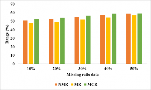
Table 3. Average RMSE of imputation for missing data when applying class labels C1 through C5
|
Missing Ratio |
NMR |
MR |
MCR |
|
10% |
50.95 |
47.73 |
52.58 |
|
20% |
52.60 |
49.43 |
54.34 |
|
30% |
55.25 |
52.11 |
56.70 |
|
40% |
57.33 |
54.57 |
59.03 |
|
50% |
58.94 |
57.26 |
59.22 |
Table 3 above represents the diverse imputation approaches using class labels C1 and C5 for different missing designs. In 10% of the missing ratio, NMR reached 50.95, MR reached 47.73, and MCR reached 52.58, respectively. 20% of the missing ratio of NMR reached 52.60, MR reached 49.43, and MCR reached 54.34. In 30%, the missing ratio of NMR reached 55.25, MR reached 52.11, and MCR reached 56.70, respectively. In 40% of the missing ratio, NMR reached 57.33, MR reached 54.57, and MCR reached 59.03, respectively. In 50% of the missing ratio, NMR reached 58.94, MR reached 57.26, and MCR reached 59.22, respectively as shown in Figure 6.
Figure 6. Graphical analysis for missing ratio data by using proposed model
A novel RL-based RNN distributed control strategy is created in order to address the problem of controlling traffic at intersections. The method uses an implanting from a traffic forecast perfect to represent a portion of the intersection's current state and forecast future traffic levels in the area. Furthermore, it is observed that they are more tolerant of changes in cycle time. Because they offer accurate information on the volume of traffic, loop detectors are essential to the success of intelligent traffic management systems. However, these systems' effectiveness is lowered because of gaps in the traffic volume data that these detectors collect. The majority of imputation techniques in use do not improve the accurate real data collected by the loop indicators. In this study, we use a data enrichment strategy to present an effective imputation approach to EIM-LD. First, two distinct datasets are created, one without noise or gaps and the other with them filled in. Subclass labels have been statistically added to the unannotated dataset. The dataset of missing volumes is then given labels using the best data model created by the RL-based RNN model. It is challenging to identify the classes in the statistical multi-class labelling procedure. Through a series of pretests, the number of courses and their volume variations were manually determined for this study. The ideal classes may be automatically found in subsequent efforts using continuous and binary metaheuristic algorithms, leading to more precise data models.
Investigation of the integration of different machine learning techniques, such as combining RNNs with reinforcement learning, to capture both temporal dependencies and complex decision-making.
[1] Ning, Z., Zhang, K., Wang, X., Obaidat, M.S., Guo, L., Hu, X., Hu, B., Guo, Y., Sadoun, B., Kwok, R.Y. (2020). Joint computing and caching in 5G-envisioned Internet of vehicles: A deep reinforcement learning-based traffic control system. IEEE Transactions on Intelligent Transportation Systems, 22(8): 5201-5212. https://doi.org/10.1109/TITS.2020.2970276
[2] Qureshi, K. N., Din, S., Jeon, G., Piccialli, F. (2020). Internet of vehicles: Key technologies, network model, solutions and challenges with future aspects. IEEE Transactions on Intelligent Transportation Systems, 22(3): 1777-1786. https://doi.org/10.1109/TITS.2020.2994972
[3] Damera, V.K., Vatambeti, R., Mekala, M.S., Pani, A.K., Manjunath, C. (2023). Normalized attention neural network with adaptive feature recalibration for detecting the unusual activities using video surveillance camera. International Journal of Safety & Security Engineering, 13(1): 51-58. https://doi.org/10.18280/ijsse.130106
[4] Garg, S., Guizani, M., Liang, Y.C., Granelli, F., Prasad, N., Prasad, R.R.V. (2021). Guest editorial special issue on intent-based networking for 5G-envisioned internet of connected vehicles. IEEE Transactions on Intelligent Transportation Systems, 22(8): 5009-5017. https://doi.org/10.1109/TITS.2021.3101259
[5] Xu, X., Zhang, X., Liu, X., Jiang, J., Qi, L., Bhuiyan, M.Z.A. (2020). Adaptive computation offloading with edge for 5G-envisioned Internet of connected vehicles. IEEE Transactions on Intelligent Transportation Systems, 22(8): 5213-5222. https://doi.org/10.1109/TITS.2020.2982186
[6] Lin, K., Li, Y., Deng, J., Pace, P., Fortino, G. (2020). Clustering-learning-based long-term predictive localization in 5G-envisioned Internet of connected vehicles. IEEE Transactions on Intelligent Transportation Systems, 22(8): 5232-5246. https://doi.org/10.1109/TITS.2020.2997472
[7] Anwar, M.R., Wang, S., Akram, M.F., Raza, S., Mahmood, S. (2021). 5G-enabled MEC: A distributed traffic steering for seamless service migration of internet of vehicles. IEEE Internet of Things Journal, 9(1): 648-661. https://doi.org/10.1109/JIOT.2021.3084912
[8] Macherla, H., Kotapati, G., Sunitha, M.T., Chittipireddy, K.R., Attuluri, B., Vatambeti, R. (2023). Deep learning framework-based chaotic hunger games search optimization algorithm for prediction of air quality index. Ingénierie des Systèmes d’Information, 28(2): 433-441. https://doi.org/10.18280/isi.280219
[9] Kong, X., Gao, H., Shen, G., Duan, G., Das, S.K. (2021). FedVCP: A federated-learning-based cooperative positioning scheme for social internet of vehicles. IEEE Transactions on Computational Social Systems, 9(1): 197-206. https://doi.org/10.1109/TCSS.2021.3062053
[10] Ning, Z., Zhang, K., Wang, X., Guo, L., Hu, X., Huang, J., Hu, B., Kwok, R.Y.K. (2020). Intelligent edge computing in internet of vehicles: A joint computation offloading and caching solution. IEEE Transactions on Intelligent Transportation Systems, 22(4): 2212-2225. https://doi.org/10.1109/TITS.2020.2997832
[11] Wang, R., Zhao, L. (2022). Application of Anti-collision early warning system for 5G internet of vehicles. In Innovative Computing. Lecture Notes in Electrical Engineering, Springer, Singapore. https://doi.org/10.1007/978-981-16-4258-6_84
[12] Kong, X., Duan, G., Hou, M., Shen, G., Wang, H., Yan, X., Collotta, M. (2022). Deep reinforcement learning-based energy-efficient edge computing for Internet of vehicles. IEEE Transactions on Industrial Informatics, 18(9): 6308-6316. https://doi.org/10.1109/TII.2022.3155162
[13] Zhu, D., Bilal, M., Xu, X. (2021). Edge task migration with the 6G-enabled network in the box for cyber twin-based Internet of vehicles. IEEE Transactions on Industrial Informatics, 18(7): 4893-4901. https://doi.org/10.1109/TII.2022.3155162
[14] Ahmad, I., Kalsoom, N., Khalid, S., Ahmed, Z. (2022). Quality of service enabled resource scheduling for cooperative driving provision in the Internet of vehicles. International Journal of Mobile Communications, 20(5): 507-518. https://doi.org/10.1504/IJMC.2022.125424
[15] Xu, X., Huang, Q., Zhu, H., Sharma, S., Zhang, X., Qi, L., Bhuiyan, M.Z.A. (2020). Secure service offloading for internet of vehicles in SDN-enabled mobile edge computing. IEEE Transactions on Intelligent Transportation Systems, 22(6): 3720-3729. https://doi.org/10.1109/TITS.2020.3034197
[16] Dangi, R., Lalwani, P., Mishra, M.K. (2023). 5G network traffic control: A temporal analysis and forecasting of cumulative network activity using machine learning and deep learning technologies. International Journal of Ad Hoc and Ubiquitous Computing, 42(1): 59-71. https://doi.org/10.1504/IJAHUC.2023.127766
[17] Dangi, R., Lalwani, P. (2023). A novel hybrid deep learning approach for 5G network traffic control and forecasting. Concurrency and Computation: Practice and Experience, 35(7): e7596. https://doi.org/10.1002/cpe.7596
[18] Lacava, A., Polese, M., Sivaraj, R., Soundrarajan, R., Bhati, B.S., Singh, T., Zugno, T., Cuomo, F., Melodia, T. (2023). Programmable and customized intelligence for traffic steering in 5G networks using open ran architectures. IEEE Transactions on Mobile Computing, 1-16. https://doi.org/10.1109/TMC.2023.3266642
[19] Ahmed, A.A., Malebary, S.J., Ali, W., Barukab, O.M. (2023). Smart traffic shaping based on distributed reinforcement learning for multimedia streaming over 5G-VANET communication technology. Mathematics, 11(3): 700. https://doi.org/10.3390/math11030700
[20] Bojović, B., Lagén, S., Koutlia, K., Zhang, X., Wang, P., Yu, L. (2023). Enhancing 5G QoS management for XR traffic through XR loopback mechanism. IEEE Journal on Selected Areas in Communications, 41(6): 1772-1786. https://doi.org/10.1109/JSAC.2023.3273701
[21] Kavehmadavani, F., Nguyen, V.D., Vu, T.X., Chatzinotas, S. (2023). Intelligent traffic steering in beyond 5G open RAN based on LSTM traffic prediction. IEEE Transactions on Wireless Communications, 22(11): 7727-7742. https://doi.org/10.1109/TWC.2023.3254903
[22] Habib, M.A., Zhou, H., Iturria-Rivera, P.E., Elsayed, M., Bavand, M., Gaigalas, R., Ozcan, Y., Erol-Kantarci, M. (2023). Hierarchical Reinforcement Learning Based Traffic Steering in Multi-RAT 5G Deployments. arXiv preprint arXiv:2301.07818. https://doi.org/10.48550/arXiv.2301.07818
[23] Wu, J., Liu, C., Tao, J., Liu, S., Gao, W. (2023). Hybrid Traffic scheduling in 5G and time-sensitive networking integrated networks for communications of virtual power plants. Applied Sciences, 13(13): 7953. https://doi.org/10.3390/app13137953
[24] Gómez, J.A.G. (2023). A cyber-physical systems approach to collaborative intersection management and control. Doctoral dissertation, Pontificia Universidad Catolica de Chile (Chile).
[25] List, G.F., Cetin, M. (2004). Modeling traffic signal control using Petri nets. IEEE Transactions on Intelligent Transportation Systems, 5(3): 177-187. https://doi.org/10.1109/TITS.2004.833763
[26] Inoue, M., Inoue, S., Nishida, T. (2018). Deep recurrent neural network for mobile human activity recognition with high throughput. Artificial Life and Robotics, 23: 173-185. https://doi.org/10.1007/s10015-017-0422-x
[27] Gouran, P., Nadimi-Shahraki, M.H., Rahmani, A.M., Mirjalili, S. (2023). An effective imputation method using data enrichment for missing data of loop detectors in intelligent traffic control systems. Remote Sensing, 15(13): 3374. https://doi.org/10.3390/rs15133374
[28] Christantonis, K., Tjortjis, C., Manos, A., Filippidou, D.E., Mougiakou, Ε., Christelis, E. (2020). Using classification for traffic prediction in smart cities. In Artificial Intelligence Applications and Innovations. AIAI 2020. IFIP Advances in Information and Communication Technology, Springer, Cham. https://doi.org/10.1007/978-3-030-49161-1_5
[29] Pasindu, H.R., Gamage, D.E., Bandara, J.M.S.J. (2020). Framework for selecting pavement type for low volume roads. Transportation Research Procedia, 48: 3924-3938. https://doi.org/10.1016/j.trpro.2020.08.028
[30] Fernandez, R., Valenzuela, E., Casanello, F., Jorquera, C. (2006). Evolution of the TRANSYT model in a developing country. Transportation Research Part A: Policy and Practice, 40(5): 386-398. https://doi.org/10.1016/j.tra.2005.08.008