Najat M. Ramadhan*![]() | Safanah M. Raafat
| Safanah M. Raafat![]() | Ali M. Mahmood
| Ali M. Mahmood![]()
© 2024 The authors. This article is published by IIETA and is licensed under the CC BY 4.0 license (http://creativecommons.org/licenses/by/4.0/).
OPEN ACCESS
Wireless Sensor Networks (WSNs) face the critical challenge of reducing node energy consumption to extend network lifetimes in the presence of uncertainties and external disturbances. This paper proposes an event-based PID controller to minimize power consumption while maintaining required data rates in WSNs. Initially, the system is stabilized using a simple controller. Two structures are considered for this purpose: one based on state feedback control and the other utilizing a PID controller. The event-based PID controller is then developed to improve the WSN system's performance and reduce power consumption. The performance of the event-based PID-controlled system is evaluated for both structures. Results with the first structure show moderate improvements in settling time, overshoot, and error, with values of 9.78 sec, 0, and 9.715, respectively. Subsequently, significant enhancements are observed with the second structure of the event-based PID controller, incorporating a stabilizing PID controller. The results demonstrate a settling time of 0.0924 sec, overshoot of 3.58, and error of 0.01486. To further enhance the controlled system's performance, the Gray Wolf Optimization (GWO) method is applied to fine-tune the parameters (P, I, and D) of the implemented controllers. The application of the GWO algorithm maintains desirable characteristics, with settling time, overshoot, and error values of 7.7527 sec, 0.0358, and 6.4217, respectively. This research offers valuable insights for reducing power consumption and improving the performance of WSNs using an event-based PID controller and GWO optimization.
wireless sensor network, power consumption, power optimization, control systems, Gray Wolf Optimization, rate control, event-based PID
In general, WSN is an infrastructure that senses and controls things using a collection of wirelessly communicating tiny embedded sensors that work together to coordinate data gathered at a central place and track the environment. The WSN is one form of sensor technology that can be used to transmit data to the base station throughout the network to keep a monitor on physical or environmental requirements like sound, temperature, movement, and pressure [1]. Other applications used to the monitoring system use the ZigBee protocols based on IEEE 802.15.4 report as an effective communication link to detect/monitor the pipeline health state by measuring the pipe's vibration and then performing data relay and data collection to send the measurements wirelessly to a centralized PC station [2]. WSNs consist of several nodes that are grouped in a specific region for collecting and transmitting the data to the main node in the network known as the sink node for special objectives such as detection and monitoring. The main point is to keep the energy consumption of data transmission and collection at a minimum level. A sensor node, cluster head, and base station are the three key components of a WSN as shown in Figure 1. The processing of WSNs is the data is sent from the sensor node to the head of the cluster node, which then sends it to the BS for more transmission. The sensor node building into four units sensing unit, a communication unit, a computing unit, and a power supply unit the process of the data happened in the computing unit, and it has an energy-consuming process. The event-based controller must be used in this situation to limit data transfer as much as feasible while still preserving energy. WSNs can be implemented using one of three topologies (Star, Tree, and Mesh). The key issues with wireless visual sensor networks, with an emphasis on the issue of energy consumption as the primary design element. It is discovered that many different forms of research on energy usage are only being started and that the primary study concern in WVSNs is power pricing [3].
Figure 1. A general schematic of WSN
There are several reasons for wasting energy in WSN, one of them failing in the network failing the sender or receiver in the network, or failing in the channel. Another reason that occurred is when there is a collision that occurred when two nodes transmit at the same time and all packets in a collision are corrupt that must be retransmitted again. On the other hand, overhearing is a third reason when a node receives packets from other nodes [4]. The Energy Threshold RPL (ETRPL) protocol is used. ETRPL relies on a novel goal function to improve the RPL protocol's energy usage by accounting for the remaining energy of the desired parent node [5]. WSNs have a fixed amount of energy to provide to the system. The key source of energy loss in WSN is idle mode consumption. Retransmission of packets is another source of energy loss in WSN. Agriculture, health care, home management, and medical applications are all available with WSN [6]. The most pressing concerns to address are how to reduce node energy consumption so that network lifetimes can be extended to realistic durations in the face of uncertainties and external disruptions. There is an urgent need to reduce power consumption while maintaining the required data speeds in WSNs.
Regarding the related works, energy saving in WSN has been considered by several pieces of literature, which are briefly described as follows. Han et al. [7] investigated the energy minimization techniques in mobile WSN, where the main focus is on the node and cluster head distribution. Likewise, Kannadhasan et al. [8] used the minimum spanning tree to find the shortest path in sensor nodes. This allows the transmitting of sensed data to the nearest base station by allowing the nodes to directly sense sensitive information to cluster heads rather than having to go through their immediate neighbors. Nayak and Devulapalli [9] proposed to use of the fuzzy logic principle for an energy-efficient clustering algorithm in WSNs. One supercluster head is elected among the cluster heads as the representative for transmitting the message to a mobile base station by selecting appropriate fuzzy descriptors. Anastasi et al. [10] used the duty cycle and data-driven methods, the networking subsystems are the center of the duty cycle. When communication is not necessary, the radio transceiver is put into sleep mode, and data-driven technology can be used to increase energy efficiency. In addition, Singh et al. [11] employed techniques that were inspired by nature to account for the short sensor life in WSNs. By comparing two optimization algorithms the Improved Genetic Algorithm and Binary Ant Colony Algorithm (IGABACA) and Lion Optimization (LO) this method can obtain the network's ideal coverage. According to the comparison, Lion Optimization (LO) outperforms IGABACA in both quality and speed. Rezaei et al. [12] used both traditional and contemporary methods to address the lifetime of WSNs. They divided this protocol into categories based on the network's structure, the way data is transferred, whether or not location data is used, and whether or not multiple pathways or Quality of Service (QoS) are maintained. Yu [13] presented the selection of cluster head construction limitations of the LEACH clustering methods, which are addressed by using software engineering techniques and presenting a novel fault-tolerant, power-efficient methodology to increase network lifetime and reduce power consumption in WSN. For the WSN to have a fault tolerance system with high fault detection probability and low fault warning probability, care should be taken to prevent failures. For instance, setting a threshold level of power consumption for each process to prevent any errors of draining the entire available power is one such careful step that should be taken. Al-Hilfi et al. [14] provided both a Particle Swarm Optimization (PSO) method for selecting the Cluster Head (CH) and a field deployment plan for clusters of deployed nodes. The procedure chooses the best CHs for cluster nodes using a fitness function. To show how to implement the suggested PSO algorithm to extend the lifespan of a WSN, this study replicates a case study for the early detection of forest fires. Another group of researchers has investigated the joint model exenterated using different controllers as follows. Han et al. [15] proposed wireless communication networks need adaptive fault-tolerant power and rate management due to transmitter flaws, parameter uncertainty, and restricted external disturbances. The parameters of the adaptive fault-tolerant controller are dynamically changed by the online estimates of possible faults to take into account the effects of network problems. Han et al. [16] proposed a fault-tolerant $H_{\infty}$ power and rate controller, where the parameters of the controller are automatically adjusted based on online estimates of future faults to account for the network's fault impact via dynamic output feedback when transmutation current problems arise. An adaptive $H_{\infty}$ was proposed by Han et al. [17], where power and rate regulation is necessary for wireless networks with time-varying unpredictability. Based on an adaptive control strategy and a reliable $H_{\infty}$ control method, a new power and rate control algorithm with dynamic output feedback is used. The linear matrix inequality is used to assess the closed-loop system's adaptive $H_{\infty}$ performance (LMI). Raafat and Mahmood [18] designed a robust control system for energy minimization. The controller is based on Model Predictive Control (MPC), and the state feedback control law which is generated by addressing an optimization problem for wireless networks with time-varying delays and input restrictions established using linear matrix inequality. The paradigm of control known as event-based control is one that naturally results from human behavior. The fundamental idea is that of an event, which can be defined as everything that takes place in the system and demands a reaction. An event-based control is used when a situation arises in the system that calls for a response. As compared to alternative strategies like analog control, which is updated continuously, and digital control, which is updated irregularly with a set time base, this distinction is significant. When some variables exceed predetermined thresholds or when events occur, the control law is changed.
In terms of event-based control, many research studies have been conducted. Åarzén [19] designed a simple event-based Proportional-Integral-Derivative (PID) controller that uses large CPU utilization reductions with a barely perceptible impact on control performance. The control method must take the varying sample interval into account, it has also been demonstrated. The suggested controller was also put to the test using a lab tank approach. For stable first-order systems, Tiberi et al. [20] suggested designing an event-based PI control architecture. A new trigger that establishes transmission instants by calculating the PI control signal was proposed.
The side effects of earlier event-triggered PI suggestions that are brought on by the process output are addressed by this approach. Abdelaal et al. [21] proposed an event-based control that was suggested as a cloud service. The goal was to understand how migrating to the cloud may save costs and save time, in addition to better utilizing the resources of the control system and conserving energy. Durand and Marchand [22] suggested ways to enhance event-based PID controllers to limit the number of samples obtained during transients, the original enhancement used a limited sampling interval condition. The second is motivated by the need to drastically reduce the error margin during steady-state intervals. PID controllers with event-based minimal computational costs and good performance have been created based on these ideas.
In this paper, the event-based PID control based on the GWO algorithm is proposed. Event-based PID control is utilized to address the power consumption issue in WSNs since it interacts with peripheral acts, makes a choice, and then executes around it. The goal is to reduce the consumed power by making the actual Signal-to-Interference-and-Noise Ratio (SINR) at a minimum value. Hence, one of the methods for reducing power usage is to apply the event-based PID controller in WSN using the mathematical model of power and rate management in WSN as explained in the next section. The main contribution is presented by using the event-based PID control based on two different stabilizing control structures to minimize the energy in the WSN. The application of the GWO algorithm in this type of system is the second key contribution of this work.
The structure of the paper is as follows. Section 2 presents the detail of the WSN network model. In section 3, the proposed event-based PID controller is developed. Section 4 illustrates the design GWO algorithm. In section 5, the simulation result is demonstrated. Finally, section 6, shows the conclusion.
In WSNs, it is critical to consider the trade-off between power consumption and data transmission speeds in addition to congestion levels [23]. Maintaining the minimal value of the actual SINR with its targeted value will allow you to reduce the amount of power consumed while simultaneously increasing the transmitted rate. As a result, the following references [18, 24-26] contain the mathematical model:
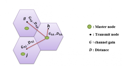
As shown in Figure 2, the master node, the active node, and the interfacing node are the three main types of nodes that make up the network topology of WSNs. The master node has access to its control inputs for the dynamic power and rates at the preceding level as well as its output measurements, while the active node h, which is found inside the master node's cell in addition, the nodes which are found in other cells and their communication representing obstructions to node h are interfacing nodes. Every node’s data must be received and processed by the master node. The interfacing nodes h and g are located in other cells and operate as barriers to the node’s communication. The following equation can be used to calculate the SINR level for nod h.
$Y_h(n)=\frac{G_{h h}(n) p(n)}{\sum g \in F G_{h g}(n) p(n)+\varphi_h^2(n)}$ (1)
where, Yh(n) is the real SINR of the h node, Ghh represents the channel gain for nodes gth to hth, p the power of transmission of node, $\varphi_h^2$ refers to a power of white Gaussian noise, F is set of closer nodes. The flow-rate control calculation used by each network node is predicted to be used by the power rate fh(k+1).
$f_h(n+1)=f_h(n)+\eta\left[d_r(n)-c(n) f_h(n)\right]$ (2)
where, fh(n) symbolizes a flow data rate of node h, $\eta$ denotes the positive step size, dr(n) depicts a gauge of network congestion, and c(n) regulates the amount of rising rate at each iteration. Eq. (3) can be used to calculate the desired SINR ($Y_h{ }^{\prime}(n)$) level for the desired data rate using Shannon's capacity formula.
$f_h(n)=\frac{1}{2} \log _2\left[1+Y_h{ }^{\prime}(n)\right]$ (3)
The state space of the model can consider in Eq. (4).
$\left.\begin{array}{c}X_d(n+1)=A x_d+B \mu_d(n)+w_d \\ S_d=C x_d\end{array}\right\}$ (4)
where,
$\begin{gathered}A=\left[\begin{array}{cc}1-\alpha & \alpha \\ 0 & 1-\eta c(n)\end{array}\right], B=\left[\begin{array}{c}E_p \\ E_f\end{array}\right], \\ C=\left[\begin{array}{ll}1 & 0 \\ 0 & 1\end{array}\right], w_d=\left[\begin{array}{c}\lambda(n) \\ \eta^{\prime} d(n)\end{array}\right]\end{gathered}$ (5)
The detailed mathematical model of WSN can be shown in [24].
Figure 2. A schematic representation of a wireless sensor network [24]
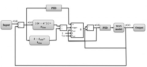
Event-based control is a control paradigm that emerges spontaneously from the way people behave. The essential concept is that of an event, which is anything that occurs in the system and necessitates a response in some way [27]. When something occurs in the system that necessitates an action, it is referred to as event-based control. Two components of the event-based PID controller are shown in Figure 3. Level crossings are detected by the time-triggered event detector in the first component on the right. The second component, which calculates the control signal, is an event-triggered PID controller [19]. The following are explanations of these:
Figure 3. The structure of event PID controller [19]
3.1 Time-triggered event detector
An event detector is used to detect level crossings. The level crossing is replaced by discretization in the amplitude in place of periodic sampling. With a period of t, this initial part is sampled regularly (much like the analogous traditional time-triggered PID). Typically, it functions as a zero-order holding which is a mathematical simulation of a typical digital-to-analog converter's (DAC) actual signal reconstruction. The holding moments, on the other hand (afterward called events), are not consistent throughout time and are determined concerning the input kinetics Thus, the event logic's objective is to establish the order of events. The input is then included in the output. The signal is constant in the interval between two events. Moreover, demand is created for each occurrence to begin the next part (i.e., the PID controller that is triggered by an event) [28].
An event occurs: either when the relative measurement exceeds a specific level.
$\left|\left(e-e_{ {old }}\right)\right|>\mathrm{e}_{\text {lim }}$ (6)
or if the maximum sample duration has been reached, at that point.
$t-t_{ {old }} \geq t_{\lim }$ (7)
where, elim is the limit value of the error, e denotes the present error, while eold denotes the former error value. t is the time span under consideration, told is the sample period's final value, and tlim is its limit value.
3.2 Event-triggered PID controller
The control signal is calculated and updated in the second section. only when a request from the first component is made, or when the event detector detects an event. The number of consecutive occurrences determines how long the (variable) sample intervals hact are. The control signal does not change during the hnom interval [19].
By reducing the data rate and the degree of congestion in WSNs, the event-based PID controller helps to minimize energy usage. If the closed-loop system is stable, this controller will only be in operation when the active trigger occurs.
A standard PID controller, whose transfer function is generally given in Eq. (8).
$u(s)=K_P+K_I \frac{1}{s}+K_D S$ (8)
3.3 The benefits of using an event-based PID controller in WSNs
The event PID controller is employed to reduce the data rate and the degree of congestion in WSNs to minimize energy consumption. If the closed-loop system is stable, this controller will only be in operation when the active condition is met. To maintain the stability of the system, this paper uses two configurations: the structure of a state feedback controller, illustrated in Figure 4, and the structure of a PID controller, displayed in Figure 5. The following sentences will explain these structures:
Figure 4. The PID / state feedback controller's organizational structure
Figure 5. The structure of event-based PID \ stabilizing PID controller
4.1 The structure of state feedback controlled system
The event PID that used a stabilizing state feedback controller is shown in Figure 4. To choose the right values for the feedback control system, the pole placement approach is used. The pole placement method is an efficient theoretical approach for managing a linear plant.
4.2 The structure of PID controlled system
The event-based PID that used a stabilizing PID controlled system is demonstrated in Figure 5. Routh-Hurwitz criterion has been used to properly select the PID parameters that guarantees the stability of the linear system.
It is important to note that all parameter values (PID gains and state feedback gain) are positive and can be properly selected to improve the performance of the WSN. Nevertheless, an optimization algorithm such as GWO can be utilized to ensure reaching the best values for an experiment as will be described in Section 5.
It can be noticed that, the event-based PID controller is used to keep the energy consumption at a minimum by minimizing the data rate along with the level of congestion. This controller will only be active at the time when the active condition is true, providing that the closed loop system is stable.
5.1 Background and motivation of GWO
The author first put up the idea of GWO in reference [29]. The behavior of the grey wolves in reference [30] served as the inspiration for the GWO concept. The concept of this algorithm came from the grey wolf’ good leadership and hunting technique where each member of the population is assigned to the position of a grey wolf, which is in a pack of 8-12.
5.2 The hierarchy of the wolves in GWO
The hierarchy is classified into four parts of the grey wolf in each group. Alpha α, beta β, omega ω and delta δ. Alpha α is also named the dominant wolf, and it is only allowed to mate with other members of the pack, the beta β wolves support the alpha in decision-making and other pack responsibilities, The delta (δ) wolf is the most vocal subspecies of the beta wolf, which dominates the omega wolf, and includes wolves such as spies, hunters, elders, and caretakers. Finally, the omega (ω) wolf is the pack's last wolf. In the case of a hunt, these wolves are the backbone of the upper-level wolves. The corresponding mathematical models for this process as presented in reference [30].
5.3 The main steps of the GWO algorithm
First: Encircling the prey: grey wolves encircle the prey during the hunt, as previously stated. The following equations are presented to mathematically model the encircling behavior.
Second: Hunting: Grey wolves can locate and encircle their prey. The alpha is usually in charge of the hunt. Hunting is something that the beta and delta might do on occasion.
Third: Searching the prey: The grey wolf diverges its position in this search process based on the present positions of the three best solutions α, β, and δ.
$\vec{Z} \vec{G}$ are the vectors that GWO uses to encircle its target, and they are calculated as follows:
$\vec{Z}=2 \vec{b} \cdot \vec{v}-\vec{b}$ (9)
$\vec{G}=2 \vec{v}_2$ (10)
In addition, to update the positions under the best search agents (which are dispersed in random ways from a central location move around the search area and communicate) position by the equations below:
$\begin{gathered}\vec{D}_\alpha=\left|\vec{G}_1 \cdot \vec{X}_\alpha-\vec{X}\right|, \vec{D}_\beta=\left|\vec{G}_2 \cdot \vec{X}_\beta-\vec{X}\right|, \vec{D}_\delta=\left|\vec{G}_3 \cdot \vec{X}_\delta-\vec{X}\right|\end{gathered}$ (11)
$\begin{gathered}\vec{X}_1=\vec{X}_\alpha-\vec{Z}_1 \cdot\left(\vec{D}_\alpha\right), \vec{X}_2=\vec{X}_\beta-\vec{Z}_2 \cdot\left(\vec{D}_\beta\right), \vec{X}_3=\vec{X}_\delta-\vec{Z}_3 \cdot\left(\vec{D}_\delta\right)\end{gathered}$ (12)
$\vec{X}=\frac{\vec{X}_1+\vec{X}_2+\vec{X}_3}{3}$ (13)
where, $\vec{D}_\alpha \vec{D}_\beta \vec{D}_\delta$ depicts the vector of the distance between the position of α, β, δ and ω. $\vec{X} \vec{G}_1 \vec{G}_2$ and $\vec{G}_3$ depicts the coefficient vectors, which have values ranging from 0 to 2. $\vec{Z}_1, \vec{Z}_2$ and $\vec{Z}_3$ is another coefficient parameter with different values that fluctuates in the range of (-1, 1).
The GWO algorithm is used in conjunction with two cost functions to enhance the performance of the regulated system. Both of the Integral Absolute Error and the control signal u (IAEU) were applied in the first scenario as shown below [31]:
$\cos t=\int\left(m_1|e(t)| d t+m_2 u(t)\right) d t$ (14)
The following equation illustrates the use of the Integral Square Error and the Control Signal u (ISEU) in the other instance from [32]:
$\cos t=\int\left(m_1|e(t)| d t+m_2 u^2(t)\right) d t$ (15)
where, m1 and m2 are constants that the try-and-error optimizer chooses.
The GWO algorithm is shown in the flowchart in Figure 6.
Figure 6. The flowchart of the GWO algorithm
The WSN presented in Eq. (5) is simulated using MATLAB using the simulation parameters shown in Table 1. The first step is achieved by studying the stability of the system using the concept of bode plot and root locus. The result in Figure 7 shows that the WSN's bode plot indicates that the system is unstable. Figure 8 uses the root locus plot to show the same result as well. In this paper, the design of the WSN-controlled system will be explained using four methods: first, the application of WSN with only PID controller. Second, using event-based PID based on state feedback and PID control structures. Third, the optimized event-based PID with the GWO algorithm is used in two scenarios to determine the best parameter values. Finally, an illustration of the event based PID based on PID control structure.
Table 1. System simulation parameters [32]
|
Parameters |
Description/Values |
|
Desired SINR |
20 dB |
|
α |
Zero mean Gaussian random variable with variance $\sigma_{\propto}^2$/0.2 |
|
C |
The amount of congestion /0.5 |
|
SpSf |
1 |
|
desired rate |
10M/s |
|
$\boldsymbol{\mu}^{\prime}$ |
0.8 |
|
n(k) and d(k) |
Zero mean with variance /0.01 |
Figure 7. The system bode plot
Figure 8. System model root locus
6.1 Stability analysis of the PID-controlled system
Figure 9 illustrates the bode plot for the system using only a PID controller, and Figure 10 displays the root locus. Then, the event based PID is constructed based on two ways; the state feedback and PID controller.
Figure 9. Bode plot with PID controller
Figure 10. The root locus of the PID control system
It is evident from Figures 9 and 10 that the PID system is generally unstable. Although the WSN is improved, it is still unstable. The event based PID can be used to enhance it. Figure 11 illustrates the Bode plot while Figure 12 demonstrates root locus of the event based PID/state feedback controller.
Figure 11. Bode plot with event based PID and state feedback control
Figure 12. Root locus with event based PID and state feedback control
Another approach is the stability of the structure of event based PID / PID. The bode plot of the PID / PID is displayed in Figure 13, whereas the root locus plot is shown in Figure 14.
Figure 13. The bode plot of the event PID / PID
Figure 14. Root locus with event based PID / PID
The two structures have improved the system's stability, as seen in Figures 11 to 14.
6.2 The WSN with event-based PID / state feedback control
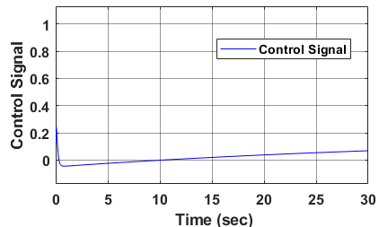
The conditions that cause the event and consequently result in the triggering action are selected first as follows; elim=0.01 and tlim=0.5. The PID parameters are selected as P=0.1, I=90, D=0.01, and the filter coefficient N=10. Figures 15 and 16 depict the SINR signal and the event monitor, respectively, while Figure 17 depicts the control signal. It is worth stating that from a control point of view, the improvement in settling time, overshoot, and steady-state error reflects the good behavior of the system to approach the desired SNR values. On the hand, from a networking point of view, keeping the SNR at a stable value means that the corresponding transmission power is also stable on the specified level which eventually improves the energy of the node and the entire network. In addition, the application of the event based control will eventually reduce the required time of calculations to only at the times of the events. That will also help in reducing the power consumption.
Although the event based WSN system has been stabilized the performance has been seen to be slow. In order to boost and improve the regulated system's performance, the GWO has been applied, as will be illustrated in 6.3.
Figure 15. The signal of SINR of event based PID / state feedback
Figure 16. The signal of control with event based PID / state feedback
Figure 17. Comparison of the control signal of the event PID / state feedback for two cases
6.3 Optimized event-based PID / state feedback
For the event based PID / state feedback controller, the cost functions are built using two instances. First, it is focused solely on optimizing the event based PID's control parameters. The (event the parameters for PID + state feedback) were subsequently optimized.
To select the best values for event-based PID, the parameters' upper, lower, and initial values, besides the iterations number, the search argent, and the parameters' values, were chosen. This state's lowest and higher values are [0.01,500, 0.001,1] and [0.5,1000, 0.1,350], respectively. This state's initial values are [0.11,90,0.01,10], there will be 10 iterations, and there are 50 search agents initially. Moreover, m1 and m2 values should be selected, and they ought to both equal 10.
The selected gains are as follows: [0.5, 1000, 0.1, 350, 100, 100] for upper values, [0.01, 500, 0.001, 1, -100, -100] for lower values, and [0.11,90,0.01,10, -264.2824, -365.5235] are the initial gains, and the number of iterations and the search agents are the same in the optimized event PID. m1 and m2 also have the same values.
Two fitness (cost) functions that are utilized (ISEU) and (IAEU).
The very sluggish SINR signal for the event based PID is illustrated in Figure 18 by the red color. The signal reaches stability at 17.66 sec., and the dashed black color displays the improved event based PID utilizing the IAUE, which marginally enhances the SINR signal. In addition, the dashed pink color shows the optimized event based PID's state feedback for IAEU, which has a higher SINR than the optimized event based PID and is stable at 11.85 sec. The last one has a value of -0.8751 dB, which is lower than the first one's value of -1.081 dB. Contrarily, the blue color shows the ISEU-optimized event based PID, which stabilizes the system at 20.26 sec. At about 8.613 sec., the optimized event- based PID/state feedback using ISEU finally reaches the stability state as shown by the green. In comparison to the optimized event based PID in ISUE, which has a value of -0.9654 dB as opposed to -0.7689 dB, the enhanced event based PID/state feedback is improved.
Figure 18. SINR comparisons for two cases for the event-based PID and state feedback
The optimal event based PID/state feedback of ISEU, where the SINR value is low and the power of WSN is also low, is the best from the aforementioned states. The comparison of the control signal for the two cases is shown in Figure 17.
6.4 The system with event-based PID/PID controller
The SINR signal, which is very quick and represents the system's good performance and stability, is shown in Figure 19. As a result, this arrangement does not require optimization. Where the SINR value is low, the power of the WSN is also low. This system has provided good performance and does not require PID parameter optimization.
6.5 Data rate vs. SINR
Determining the data rate number using the SINR signal's specific points and the Shannon power formula in Eq. (3) was crucial. The data rate is calculated using five randomly selected SINR points, first for the event-based PID/state feedback shown in Figure 20 and then for the event-based PID/PID shown in Figure 21. Table 2 displays the SINR versus data rate for Event-based PID/state feedback and Event-based PID/PID.
Figure 19. The Signal of SINR with event based PID / PID
Table 2. Data rate vs. SINR for event-based PID / PID
|
No. |
SINR |
Data Rate |
|
Event based PID / state feedback |
||
|
1 |
-0.07514 |
0.1126931 |
|
2 |
0.1147 |
0.156655489 |
|
3 |
0.2865 |
0.363451457 |
|
4 |
0.3715 |
0.455754622 |
|
5 |
0.4548 |
0.54082083 |
|
Event based PID / PID |
||
|
1 |
0.986 |
0.98986562 |
|
2 |
0.991 |
0.993493221 |
|
3 |
0.9925 |
0.994579724 |
|
4 |
1.011 |
1.007913082 |
|
5 |
1.03 |
1.021479727 |
Figure 20. SINR against data rate for event-based / state feedback
Secondly, we display the result of the event-based PID controller. In this case, the event characteristics are selected to be elim=0.0005 and tlim=0.5, utilizing the trial-and-error procedure, the event monitor's PID parameter was chosen to be P=0.11, I=850, D=0, and N=100 for the filter coefficient, while the parameter of PID with the model which P=-37.668, I=30.561, D= 0.05269, and filter coefficient N=100. Figure 19 illustrates the SINR signal.
The next state when calculating the data rate for optimized event PID / state feedback in IAEU and ISEU. The results can be shown in Table 3 and Figures 22 and 23.
Figure 21. SINR vs. data rate with event-based PID / PID
Table 3. The SINR V.S data rate for optimized event PID / state feedback using ISEU
|
No. |
SINR |
Data Rate |
|
Optimized event PID using ISEU |
||
|
1 |
-0.9654 |
4.85308 |
|
2 |
-0.4012 |
0.73985 |
|
3 |
0.3691 |
0.453228 |
|
4 |
0.738 |
0.797428 |
|
5 |
0.9837 |
0.988194 |
|
Optimized event /state feedback using ISEU |
||
|
1 |
-0.7714 |
2.1291 |
|
2 |
-0.2121 |
0.34392 |
|
3 |
0.3507 |
0.433707 |
|
4 |
0.7069 |
0.771379 |
|
5 |
0.9798 |
0.985355 |
Figure 22. SINR against data rate for optimized event-based using IAEU
Figure 23. SINR against data rate with optimized event-based / state feedback using ISEU
Table 4 and Table 5 provided the following explanations of the traits of event-based control system before and after using the GWO, where Tr is the rise time that reflects the speed of system response to reach its desired value (the SINR), Ts is the settling time, which is the amount of time needed for the output to stabilize and reach a specific tolerance band. O.S. refers to the overshoot of the response or in other words it occurs when the signal overshoots its aim is known as overshoot, and E is the error steady state.
Table 4. The transient response characteristics of the event-based control system
|
Characteristics of the Control System |
|||||
|
Controller type |
Tr |
Ts |
O. S |
U. S |
E |
|
PID |
1.975 |
29.98 |
0 |
7.8 |
13660574.77 |
|
Event PID based on state feedback |
5.02 |
9.78 |
0 |
56.08 |
9.715 |
|
Event PID based on PID |
0.023 |
0.0924 |
3.58 |
0 |
0.01486 |
|
Characteristics of optimized event PID based on state feedback using IAEU |
|||||
|
Optimized Event PID |
3.9 |
7.93 |
0 |
1.1 |
6.111 |
|
Optimized Event PID / state feedback |
3.1896 |
7.542 |
0.1247 |
87.8 |
6.2516 |
|
Characteristics of optimized event PID based on state feedback using ISEU |
|||||
|
Optimized Event PID |
4.3996 |
8.537 |
0 |
1.011 |
6.484 |
|
Optimized Event PID / state feedback |
3.248 |
7.7527 |
0.0358 |
76.5843 |
6.4217 |
Table 5. The value of the event-based controlled system's solution parameter
|
Before Optimization |
|||||||||
|
Controller type |
P |
I |
D |
|
State feedback |
P |
I |
D |
|
|
PID |
-827.5 |
544.54 |
0 |
100 |
-- |
|
|
|
|
|
Event PID based on state feedback |
0.11 |
90 |
0.01 |
10 |
-264.2824 |
-365.523 |
-- |
||
|
Event PID based on PID |
0.11 |
850 |
0 |
-- |
-37.668 |
0.561 |
0.05269 |
||
|
The best solution of event PID based on state feedback using IAEU |
|||||||||
|
Optimized Event PID |
0.096 |
792.566 |
0.0818 |
178.6 |
-- |
-- |
|||
|
Optimized Event PID / state feedback |
0.01725 |
644.85 |
0.08815 |
93.467 |
44.764 |
56.831 |
|||
|
The best solution of event PID based on state feedback using ISEU |
|||||||||
|
Optimized Event PID |
0.086178 |
832.430 |
0.05797 |
276.2 |
-- |
-- |
|||
|
Optimized Event PID / state feedback |
0.02316 |
680.1643 |
0. 0444 |
58.1505 |
- 66.7147 |
- 82.868 |
|||
The efficient management of power consumption in Wireless Sensor Networks (WSNs) is crucial due to their deployment in challenging or inaccessible environments. By reducing node energy usage, the network lifetime can be extended, ensuring sustained operation. In this paper, we have presented the utilization of an event-based PID controller to enhance energy efficiency in WSNs. The controller is designed to optimize transmission based on the network's necessity, leading to intelligent energy usage.
Two different inner loop structures were employed in the design of the event-based PID controller: a state feedback-controlled system and a PID-controlled system. The selection of optimal controller parameters was accomplished using the Gray Wolf Optimization (GWO) algorithm, which effectively fine-tunes the controller for improved performance.
While the implementation of the event-based PID and state feedback methods may introduce a slight increase in power consumption, the event-based PID/PID approach exhibited rapid response and superior performance, requiring no further improvements. To assess the outcomes, the IAEU and ISEU cost functions were utilized for the optimization of the event-based PID/state feedback.
The results obtained through the application of the GWO algorithm demonstrated enhanced system performance. A comparison between the results based on IAEU and ISEU revealed that the latter cost function consistently maintained better performance, and the optimization of PID/state feedback using this cost function significantly improved the system's output.
In conclusion, this research has contributed to addressing the critical power consumption issue in WSNs through the utilization of an event-based PID controller. By employing the GWO algorithm for parameter optimization and selecting appropriate cost functions, substantial enhancements in energy efficiency and system performance were achieved. These findings have practical implications for designing energy-efficient WSNs and furthering the understanding of event-based control in resource-constrained environments.
[1] Dash, L., Khuntia, M. (2020). Energy efficient techniques for 5G mobile networks in WSN: A Survey. In 2020 International Conference on Computer Science, Engineering and Applications (ICCSEA), Gunupur, India, pp. 1-5. https://doi.org/10.1109/ICCSEA49143.2020.9132941
[2] Mossa, N.F., Shareef, W.F., Shareef, F.F. (2018). Design of oil pipeline monitoring system based on wireless sensor network. Iraqi Journal of Computers, Communication and Control & Systems Engineering, 18(2): 53-62. https://doi.org/10.33103/uot.ijccce.18.2.5
[3] Ahmad, I.A., Al-Nayar, M.M.J., Mahmood, A.M. (2022). Investigation of energy efficient clustering algorithms in WSNs: A review. Mathematical Modelling of Engineering Problems, 9(6): 1693-1703. https://doi.org/10.18280/mmep.090631
[4] Rezaei, Z., Mobininejad, S. (2012). Energy saving in wireless sensor networks. International Journal of Computer Science & Engineering Survey (IJCSES), 3: 23-37. https://doi.org/10.5121/ijcses.2012.3103
[5] Rafea, S.A., Kadhim, A.A. (2019). Routing with energy threshold for WSN-IoT based on RPL protocol. Iraqi Journal of Computers, Communications, Control & Systems Engineering, 19: 71-81. https://doi.org/10.33103/uot.ijccce.19.1.9
[6] Hashim, S.A., Jawad, M.M., Wheedd, B. (2020). Study of energy management in wireless visual sensor networks. Iraqi Journal of Computers, Communications, Control and Systems Engineering, 20(1): 68-75. https://doi.org/10.33103/uot.ijccce.20.1.7
[7] Han, C., Sun, D., Bi, S., Dong, Z., Lei, Z. (2013). Adaptive fault-tolerant power and rate control for wireless networks with transmitter failures and uncertainties. In 2013 25th Chinese Control and Decision Conference (CCDC), Guiyang, China, pp. 1145-1150. https://doi.org/10.1109/CCDC.2013.6561097
[8] Kannadhasan, S., Balaganesh, R., Srividhya, G. (2013). A survey on recent trends in wireless sensor networks. International Journal of Emerging Trends in Electrical and Electronics.
[9] Nayak, P., Devulapalli, A. (2015). A fuzzy logic-based clustering algorithm for WSN to extend the network lifetime. IEEE Sensors Journal, 16(1): 137-144. https://doi.org/10.1109/JSEN.2015.2472970
[10] Anastasi, G., Conti, M., Di Francesco, M., Passarella, A. (2009). Energy conservation in wireless sensor networks: A survey. Ad Hoc Networks, 7(3): 537–568. https://doi.org/ 10.1016/j.adhoc.2008.06.003
[11] Singh, A., Sharma, S., Singh, J. (2021). Nature-inspired algorithms for wireless sensor networks: A comprehensive survey. Computer Science Review, 39, 100342. https://doi.org/10.1016/j.cosrev.2020.100342
[12] Rezaei, Z., Mobininejad, S. (2012). Energy saving in wireless sensor networks. International Journal of Computer Science & Engineering Survey (IJCSES), 3: 23-37. https://doi.org/10.5121/ijcses.2012.3103
[13] Yu, Y. (2012). A survey of intelligent approaches in wireless sensor networks for efficient energy consumption. In Proceedings of the International Conference on Software and Computer Applications (ICSCA’12), pp. 144-148.
[14] Al-Hilfi, H.I.M., Al-Nayar, M.M.J. (2022). Increase the WSN-lifespan used in monitoring forest fires by PSO. Mathematical Modelling of Engineering Problems, 9(3): 583-590. https://doi.org/10.18280/mmep.090304
[15] Han, C.W., Sun, D.H., Li, Z.J., Shi, Y.T. (2014). Adaptive H∞ power and rate control for time-varying uncertain wireless networks via dynamic output feedback. Applied Mechanics and Materials, 548: 1524-1529. https://doi.org/10.4028/www.scientific.net/AMM.548-549.1524
[16] Han, C., Sun, D., Bi, S., Liu, L., Li, Z. (2014). Modeling and model predictive power and rate control of wireless communication networks. Journal of Applied Mathematics, 2014: 642673. https://doi.org/10.1155/2014/642673
[17] Han, C., Sun, D., Liu, L., Bi, S., Li, Z. (2014). Robust model predictive power and rate control for uncertain wireless networks with time-varying delays and input constraints. In Proceedings of the 33rd Chinese Control Conference, Nanjing, China, pp. 5447-5452. https://doi.org/10.1109/ChiCC.2014.6895870
[18] Raafat, S.M., Mahmood, A.M. (2021). Robust energy efficient control for wireless sensor networks via unity sliding mode. Journal of Engineering Science and Technology, 16(1): 65-84.
[19] Åarzén, K.E. (1999). A simple event-based PID controller. IFAC Proceedings Volumes, 32(2): 8687-8692. https://doi.org/10.1016/s1474-6670(17)57482-0
[20] Tiberi, U., Araújo, J., Johansson, K.H. (2012). On event-based PI control of first-order processes. IFAC Proceedings Volumes, 45(3): 448-453. https://doi.org/10.3182/20120328-3-IT-3014.00076
[21] Abdelaal, A.E., Hegazy, T., Hefeeda, M. (2017). Event-based control as a cloud service. In 2017 American Control Conference (ACC), Seattle, WA, USA, pp. 1017-1023. https://doi.org/10.23919/ACC.2017.7963086
[22] Durand, S., Marchand, N. (2009). An event-based PID controller with low computational cost. In SampTA 2009-8th International Conference on Sampling Theory and Applications. https://hal.archives-ouvertes.fr/hal-00393031.
[23] Han, C., Li, M., Liu, L., Pang, Z. (2017). Robust power and rate control for nonlinear wireless communication networks. In 2017 36th Chinese Control Conference (CCC), Chongqing, China, pp. 1097-1102. https://doi.org/10.1109/CCDC.2017.7978304
[24] Han, C., Sun, D., Bi, S., Liu, L., Li, Z. (2014). Modeling and model predictive power and rate control of wireless communication networks. Journal of Applied Mathematics, 2014: 642673. https://doi.org/10.1155/2014/642673
[25] Subramanian, A., Khajehnouri, N., Sayed, A.H. (2003). A minimum variance rate and power update algorithm for wireless networks. In 2003 IEEE 58th Vehicular Technology Conference. VTC 2003-Fall (IEEE Cat. No. 03CH37484), Orlando, FL, USA, pp. 1468-1472. https://doi.org/10.1109/vetecf.2003.1285268
[26] Subramanian, A., Sayed, A.H. (2005). Joint rate and power control algorithms for wireless networks. IEEE Transactions on Signal Processing, 53(11): 4204-4214. https://doi.org/10.1109/TSP.2005.857044
[27] Sombría, J.C. (2014). Contributions to the analysis, simulation, and experimentation on event-based PID control systems. Universidad Nacional de Educación a Distancia, Spain.
[28] Durand, S., Boisseau, B., Marchand, N., Guerrero-Castellanos, J.F. (2018). Event-based PID control: Application to a mini quadrotor helicopter. Journal of Control Engineering and Applied Informatics, 20(1): 36-47.
[29] Mirjalili, S., Mirjalili, S.M., Lewis, A. (2014). Grey wolf optimizer. Advances in Engineering Software, 69: 46-61. https://doi.org/10.4271/972882
[30] Rajakumar, R., Sivanandakumar, D., Uthayakumar, J., Vengattaraman, T., Dinesh, K. (2020). Optimal parameter tuning for PID controller using accelerated grey wolf optimisation in smart sensor environments. Electronic Government, An International Journal, 16(1-2): 170-189. https://doi.org/10.1504/EG.2020.105237
[31] Wang, Z., Wang, W. (2007). Research on algorithm of web classification based on EP and FFSS. In 2007 International Conference on Computational Intelligence and Security (CIS 2007), Harbin, China, pp. 162-166. https://doi.org/10.1109/CIS.2007.194
[32] Liu, Y., Wu, Q., Zhao, T., Tie, Y., Bai, F., Jin, M. (2019). An improved energy-efficient routing protocol for wireless sensor networks. Sensors, 19(20): 4579. https://doi.org/10.3390/s19204579