Vamsi Krishna Pappala*![]() | Rama Sudha Kasibhatla
| Rama Sudha Kasibhatla![]() | Venkata Krishna Bhanu Chennapragada
| Venkata Krishna Bhanu Chennapragada![]() | Chandra Sekhar Akkapeddi
| Chandra Sekhar Akkapeddi![]()
© 2023 IIETA. This article is published by IIETA and is licensed under the CC BY 4.0 license (http://creativecommons.org/licenses/by/4.0/).
OPEN ACCESS
India's commitment to renewable energy has been reinforced through its ranking as the fourth-largest global solar power capacity holder, as reported in the Ministry of New and Renewable Energy's 2022 year-end review. Non-fossil fuel-based power generation has reached 42.26% of India's total installed capacity. In this context, solar pump installations for agricultural use, under the component – A, B, C, are in progress. This study proposes the deployment of stand-alone solar power plants using the System Advisor Model (SAM) in three distinct regions of Andhra Pradesh, India. Aimed at facilitating the adoption of green energy and income generation through surplus power sales in rural communities, this work is grounded in a comprehensive survey conducted across eight diverse locations: Ganayigudem, Manduru, Jogannapalem, Vegavaram, Veeravallipalem, Ainavillilanka, Seetharampuram, and Naguladevupadu. Real-time power requirement data was collected from 112 farmers across approximately 882 acres of land. These locations were divided into three sets, designated as set-A, set-B, and set-C, using a clustering approach. The energy requirements for agricultural purposes were derived from the survey data, enabling the near-practical construction of a solar plant via the SAM software, using actual weather data and load requirements. The Levelized cost of energy nominal (LOCE) was calculated to be 3.38 \$/kWh and 2.7 \$/kWh per cent of land area for set-A, 3.18 \$/kWh and 2.54 \$/kWh for set-B, and 3.33 \$/kWh and 2.66 \$/kWh for set-C. These figures encapsulate the cost of constructing and maintaining the solar plant over its lifespan. The lower LOCE for set-B compared to set-A is attributed to the larger plant size in set-A. The feasibility of solar plant construction is enhanced by government-provided tax benefits. However, it is noteworthy that changes in weather patterns may introduce slight discrepancies in practical implementation, as the current results are based on past weather data.
SAM (System Advisor Model) software, energy production, solar plant, simulation, energy technologies
In this paper the focus was on development of both agriculture sector and renewable energy by improving the agriculture by supplying continuous power supply with renewables. In India, despite of COVID-19, agriculture sector had been a ray of hope in Indian economy. For improvement of GDP through agriculture was 4532.49 INR Billion, these figures made Indian government to keep a goal for improvement of agriculture sector, for this government has taken certain measures to give some incentive to agriculture sector through some schemes like, Increasing procurement from farmers, Income support to farmer through Pradhan Mantri Kisan Urja Suraksha Evam Utthaan Mahabhiyan scheme with this initiative government is going for installation of renewable energy sources with a capacity of 30,800MW by 2022. The energy policy of India is to produce energy rurally to decrease energy poverty. Generation from fossil fuel sources is 57.74% of total installed generation capacity in the country. In consideration to support GDP in an efficient way, a shift towards renewable energy generation is necessary, as they are almost inexhaustible and they emit less carbon emissions, pushing for cleaner and green climate initiative for safer environment.
To understand how to support the energy policy, literature survey had been conducted on various countries on how they are overcoming these energy issues. A survey that was done on agriculture farms in Punjab, Pakistan was collected on practical load requirement and with the help of SAM software simulation [1] on five locations Attock, Chiniot, Faisalabad, Mainwali and Multan. A 14.5kW and 145kW system analysis has been done and techno-economic details of PV plant were given by Aziz et al. [2]. A mathematical model to understand variations in temperature and radiation of solar energy with respect to five cities in Iran, analysing the variation in solar energy production in five locations with climate data with the help of SAM software and rankings were given based on performance in Ghodusinejad et al. [3]. Thailand model discusses about how battery storage system has become a drawback on customer economics and different policies all these included a 5kW SAM simulation model impact on returns and system flexibility has been given in Chaianong et al. [4]. Geographical distribution of solar generation in sites of Saudi Arabia in SAM software hourly, solar radiation patterns analysis and various losses given by Alharthi et al. [5]. Analyzed India’s solar generation through satellite-derived data of global and diffuse radiation for 23 locations in the span of 15 years gave a report of maximum and minimum radiation of 85% efficiency i.e., in Andhra Pradesh, India. For total radiation with a comparison of ground measurement and satellite derived data is in Mahima et al. [6]. Non-financial model was done by using SAM software simulation in Brazilian regions, their main aim was generation of electricity through solar energy as the region is abundant in solar radiation which helps us in capturing of solar energy implementation of 2MW of 19 power plants has done where economic analysis has not been done in Pimentel da Silva [7]. A study on designing 1.2MW commercial PV system and financial model at Abu Dhabi with SAM software has shown hourly, monthly and annually performance with system design, operating costs and installation in Alharthi et al. [5]. A study on solar panels inclination and the advantages in title angle adjustments for maximum output was discussed in Alhendal et al. [8]. A simple way of estimating a solar energy for a building including losses involved was shown in Santos et al. [9].
The literature to date has not presented a comprehensive model of a photovoltaic (PV) system specifically tailored for agricultural purposes that would enhance rural agriculture in India. Such a model would significantly benefit the environment through pollution reduction, offer economic assessments, and create income opportunities within agricultural communities, thereby mitigating rural migration. Moreover, a detailed methodology for plant construction, incorporating solar panel selection, the number of inverters, system design, and economic estimations, is lacking. The present study aims to address these deficiencies.
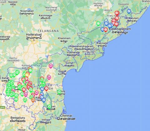
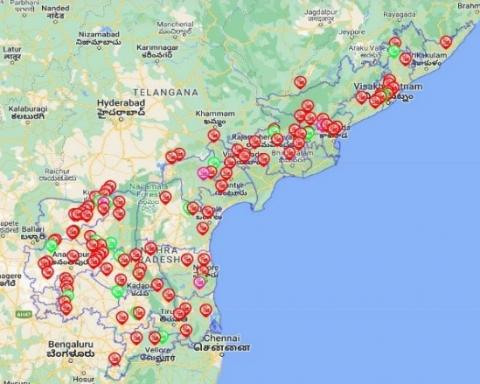
The objective is to design stand-alone PV systems for agricultural purposes across three location clusters in Andhra Pradesh, India. The intention is to augment the quality and quantity of energy supply for agricultural needs. These regions have been specifically selected due to the absence of renewable energy plants in these locations, as can be seen in Figures 1 and 2. The methodology employed in this study aims to align with current government policies. Practical data was collected from 112 farmers spanning 882 acres of land across various locations in Andhra Pradesh, India. These locations include Ganayigudem, Manduru, Jogannapalem, Vegavaram, Veeravallipalem, Ainavillilanka, Seetharampuram, and Naguladevupadu. Direct contact with farmers facilitated data collection, which encompasses information such as the farmer's location, name, land size, crop type, and motor capacity. Given their latitude, these eight locations have been divided into three sets: set-A (Ganayigudem, Seetharampuram, Vegavaram, and Ainavillilanka), set-B (Jogannapalem, Naguladevupadu, and Veeravallipalem), and set-C (Manduru). The collected data indicate that set-A, set-B, and set-C have loads of 647kW, 259kW, and 398kW, respectively. Consequently, 650kW, 300kW, and 400kW plants were constructed to supply power to these sets' agricultural fields using the SAM software. This software, provided with practical data related to weather conditions, load requirements, power selling costs, debt percentages, and land taxes, can construct optimal PV plants as will be demonstrated in the subsequent sections of this paper.
The significance of this work lies in its potential to address increased household power needs arising from the pandemic-induced shift towards remote work. The establishment of small grids powered by renewable energy sources could elevate the energy supply while reducing environmental impact. Additionally, these initiatives could create job opportunities in rural areas where the population largely depends on agriculture, thus benefiting local communities and their environs.
Figure 1. The availability of non-conventional energy sources Andhra Pradesh, India
Figure 2. The availability of conventional energy sources Andhra Pradesh, India
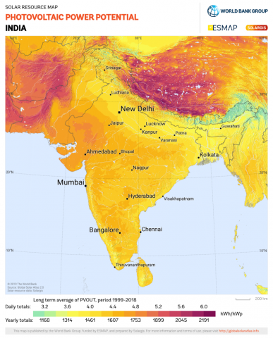
India is rich in capturing solar energy, so production of energy through PV system for agriculture needs [10] in rural areas will be benefited to government as they can reduce the production of energy through conventional resources which will help in reduction of pollution. And for rural people it helps to increase their income and opportunities. The system in SAM software contains PV modules, inverters and cables, with a detail analysis of costs involved in procuring the equipment. And the localized costs in selling power are also involved in SAM software for better economic [11-14] analysis with all losses involved. Figure 3 shows PV potential in India. India is located geographically between latitude 20.5937° N and longitude 78.9629° E. New & Renewable Energy Development Corporation of Andhra Pradesh Ltd. [15] shared the present availability of renewable and non-renewable generating stations in Andhra Pradesh state shown in Figure 1 and Figure 2, Figure 1 shows places where non-conventional energy source plants are available and Figure 2 shows places where conventional energy source plants are available.
2.1 Study locations and data collection
In India the selected locations are Ganayigudem latitude 16.7761° N and longitude 81.1458° E, Manduru latitude 16.1640° N and longitude 80.6375° E, Jogannapalem latitude 16.8150° N and longitude 81.1679° E, Vegavaram latitude 16.7666° N and longitude 81.1212° E, Veeravallipalem latitude 16.6882° N and longitude 82.0012° E, Ainavillilanka latitude 16.6772° N and longitude 82.0203° E, Seetharampuram latitude 16.7519° N and longitude 81.4289° E and Naguladevupadu latitude 16.8319° N and longitude 81.1874° E. A brief detail of eight locations were given in Table 1 where we can see latitude, longitude, solar irradiation and average temperature. In these locations a survey has been conducted from the farmers in person to person individually and parameters collected are Location, Name of the farmer, Size of land, Type of crop, Specify the duration of water requirements, Capacity of the motor, Type of the motor (1-∅ or 3-∅), Timings of power supply/day by the government and Showing interest to install PV system etc. For irradiation global radiation is considered. And coming to location satellite weather data, in SAM software have weather data option from there user can get access to various sources of solar resource data in that the source selected was PHOTOVOLTAIC GEOGRAPHICAL INFORMATION SYSTEM for this source by giving location data user can get solar resource data of that particular location then we can upload this file in SAM software to run simulation.
Figure 4 shows the location of Andhra Pradesh in India map. Figure 5 shows the eight locations which were selected in Andhra Pradesh.
Table 1. Data of selected locations
|
|
Ganayigudem |
Manduru |
Jogannapalem |
Vegavaram |
Veeravallipalem |
Ainavillilanka |
Seetharampuram |
Naguladevupadu |
|
Latitude |
16.7761 |
16.1640 |
16.8150 |
16.7666 |
16.6882 |
16.6772 |
16.7519 |
16.8319 |
|
Longitude |
81.1458 |
80.6375 |
81.1679 |
81.1212 |
82.0012 |
82.0203 |
81.4289 |
81.1874 |
|
Solar irradiation (kWh/m2/day) |
4.9899 |
5.2977 |
6.0627 |
5.2982 |
5.2967 |
5.2966 |
5.2975 |
5.2983 |
|
Average Temp. (℃) |
28.1 |
30 |
27.4 |
28 |
29.1 |
29 |
30 |
27.9 |
Figure 3. PV potential in India (http://globalsolaratlas.info)
Figure 4. The location of Andhra Pradesh in India
Figure 5. The availability of conventional energy sources Andhra Pradesh, India
2.2 System sizing and optimization
Use of SAM software, is to construct a virtual PV plant by giving all practical inputs to get practical output results by including all the parameters involved in practical PV plant. The first step in analysis is location and resource data, in this the weather file is to be uploaded so that yearly solar insolation inputs were given to SAM software for practically checking for grid construction at given location, for quicker returns. From the given weather file, the SAM software will show information as latitude, longitude, time zone and elevation in addition to this user can also see information about albedo that is the surface diffusion of earth. Next selection of the module the main important thing in a solar plant, is depending upon solar irradiance and cell temperature is to be decided very carefully because the system efficiency was depending upon module considered.
For optimal system sizes based on load for cluster-1 i.e. set-A the required was 650kW now to maintain a DC to AC ratio of 1.1 while designing a system total DC capacity should be divided with Standard Test Conditions (STC), which gives number of modules so, user have to take an STC value near to total DC capacity here the selected module was CSI Solar Co. Ltd. CS7N-645MB-AG where the specifications are given in Table 2 for set-A here the total number of modules are 1,110.
Table 2. Module details
|
Module |
|
|
CSI Solar Co. Ltd. CS7N-645MB-AG |
|
|
Cell material |
Mono-c-Si |
|
Module area |
3.07 m² |
|
Module capacity |
645.05 DC Watts |
|
Quantity |
1,110 |
|
Total capacity |
716 DC kW |
|
Total area |
3,407 m² |
|
CSI Solar Co. Ltd. CS7N-645MB-AG |
|
|
Cell material |
Mono-c-Si |
|
Module area |
3.07 m² |
|
Module capacity |
645.05 DC Watts |
|
Quantity |
510 |
|
Total capacity |
328.97 DC kW |
|
Total area |
1,565 m² |
|
CSI Solar Co. Ltd. CS7N-645MB-AG |
|
|
Cell material |
Mono-c-Si |
|
Module area |
3.07 m² |
|
Module capacity |
645.05 DC Watts |
|
Quantity |
680 |
|
Total capacity |
438.63 DC kW |
|
Total area |
2,087 m² |
Table 3. Inverter details
|
Inverter |
|
|
Custom (Inverter Part Load Curve Model) |
|
|
Unit capacity |
650 AC kW |
|
Input voltage |
310 DC V |
|
Quantity |
1 |
|
Total capacity |
650 AC kW |
|
DC to AC capacity ratio |
1.10 |
|
Custom (Inverter Part Load Curve Model) |
|
|
Unit capacity |
300 AC kW |
|
Input voltage |
310 DC V |
|
Quantity |
1 |
|
Total capacity |
300 AC kW |
|
DC to AC capacity ratio |
1.10 |
|
Custom (Inverter Part Load Curve Model) |
|
|
Unit capacity |
400 AC kW |
|
Input voltage |
310 DC V |
|
Quantity |
1 |
|
Total capacity |
400 AC kW |
|
DC to AC capacity ratio |
1.10 |
Inverter was chosen as per the load demand. In SAM software, users can choose an inverter model in four ways. They are: 1. Inverter CEC database, 2. Inverter Datasheet, 3. Inverter part load curve, and 4. Inverter CEC coefficient generator. Here, the Inverter part load curve has been taken for the analysis in SAM software because of the flexibility of design for requirements. In other methods, there are only specified ratings of inverters, which are limited for a range of values that do not match the actual or practical calculated value. The inverter was designed to supply a nominal AC voltage of 415Vac and a maximum DC voltage of 440Vdc. These will be the operating ranges as per the module open circuit voltage of 44.8Vdc. As the module per string in the sub-array was 10, then 44.8 multiplied by 10 gives nearly 440Vdc. Along with this, the DC to AC capacity ratio needs to be maintained. All the set-A, B, and C were maintained at a ratio of 1.1. Here, for set-A, inverter specifications are given in Table 3.
For cluster-2, i.e., set-B, a 300kW plant, the selected module was CSI Solar Co. Ltd. CS7N-645MB-AG. The specifications are given in Table 2. Here, the number of modules is 510, and the inverter was a custom inverter with a DC to AC ratio of 1.10. This gives a nominal AC voltage of 415v. For set-A, inverter specifications are given in Table 3.
For cluster-3, i.e., set-C, a 400kW plant, the selected module was again CSI Solar Co. Ltd. CS7N-645MB-AG. The specifications are given in Table 2. Here, the number of modules is 680, and the inverter was a custom inverter with a DC to AC ratio of 1.10. This gives a nominal AC voltage of 415v. For set-A, inverter specifications are given in Table 3.
2.2.1 System design parameters
System design in SAM software will provide us with accurate data on coupling inverter and module. In system design data, the shown details are total AC capacity, name plate DC capacity, total inverter DC capacity, number of modules, number of strings, total module area, strings in parallel sub array, string Voc at reference conditions, and tracking & orientation related terms such as tilt angle and azimuth. These details are shown in Table 4.
Table 4. System specifications
|
System Design |
|
|
All system details |
|
|
Strings |
111 |
|
Modules per string |
10 |
|
String Voc (DC V) |
448 |
|
Tilt (deg from horizontal) |
16.78 |
|
Azimuth (deg E of N) |
180 |
|
DC losses (%) |
3.47 |
2.2.2 AC capacity
Inverter Total Capacity (kWac)=Inverter Maximum AC Power (Wac)×0.001 (kW/W)×Number of Inverters
2.2.3 Inverter DC capacity
Inverter Total Capacity (kWdc)=Inverter Maximum DC Input Power (Wdc)×0.001 (kW/W)×Number of Inverters
2.2.4 Nameplate DC capacity
Nameplate Capacity (kWdc)=Module Maximum Power (Wdc)×0.001 (kW/W)×Total Modules
2.2.5 Number of modules
Total Modules=Modules per String×Strings in Parallel
2.2.6 Module area
Total Area (m²)=Module Area (m²)×Number of Modules
2.3 Techno-economic analysis
The LOCE depends on number of factors among them majority of share was from equipment, labour costs, construction period, financing costs, size of debt (amount borrowed), maintenance, insurance and property taxes.
2.3.1 Economic analysis
In SAM software user can have different type of analysis in economic perspective which gives detail analysis of plant in view of returns for sustainability
2.3.2 Annual degradation
The degradation rate is applied linearly starting in year 2. In schedule mode, each year’s rate applies to the year 1 value and also applies a daily loss to DC output and AC input are also are involved. In the entire three cases degradation rate was taken as 0.5% per annum.
2.3.3 Installation costs
The SAM software include PV capital costs in this direct capital costs involves module cost, inverter cost, balance of system equipment cost, installation labor cost and installer margin and overhead. PV capital costs also includes indirect capital costs involves permitting and environmental studies, engineering and developer overhead, grid interconnection and land costs involved in addition to this sales tax was also included by combining all these things user get total installed cost and total installed cost per capacity.
2.3.4 Operation and maintenance costs
Operation and maintenance costs includes fixed annual cost where user can give in \$/yr as first year cost and in percentage the escalation rate this software applies both inflation and escalation to the first-year cost to calculate out-year costs. It also includes fixed cost by capacity and variable cost by generation.
2.3.5 Financial parameters
Financial parameters include debt fraction which gives information about how much percentage amount was user taking for PV system construction as debt i.e., 100% loan or 50% etc. these also include loan term for all cases 25years was taken and project tax and insurance rates are also involved.
2.3.6 Electricity rates
In metering and billing user has four analyses they are net energy metering, net energy metering with \$ credits, net billing, net billing with carryover to next month and buy all/sell all in all these analysis net energy metering with \$ credits were taken and here as per Solar Energy Corporation of India (SECI) [16] government of India calls for tenders for solar plants and it will purchase at 0.03 \$/kWh and sells it for 0.12 \$/kWh these rates are included.
2.3.7 Electric load
Electric load profile data describes the electricity usage of an agriculture purposes for electricity calculations as per the loads user can scale the required output or input according to needs as per climatic conditions for all the months in every year here the load was given in energy form.
2.3.8 Electricity rates and incentives
In SAM software there is Metering and billing section here user can give rates of energy charges as per the government norms or rates, user can also sell the energy generated during peak time, user can increase the cost for getting fast returns and while in normal times user can sell power by giving incentives if there is abundant storage of energy available user can give this data hourly.
2.4 Simulation and modeling
SAM performs simulation with the help of data given to it like weather data and DC to AC requirement by selecting proper STC value user can estimate the number of modules required. And selection of inverter can be done as per requirement after this user can run simulation then SAM will show monthly data of the energy generation according to solar insolation of that month which was given as weather file at starting. Now coming to losses SAM includes all the parameters like irradiance loss, DC and AC losses and it also gives information about lifetime and degradation. All these results can get from this model by giving necessary data.
2.5 Limitations and uncertainties
The limitations and uncertainties are due to uncertain changes in weather on day-to-day and year-to-year basis the weather conditions are unpredictable so, for going to practical implementation of PV plant the output may vary based on climatic conditions. To improve this user, have to update the weather files up to date and make certain changes for better output.
As per the survey data collection from farmers set-A has a load was 647kW, set-B has a load of 259kW and set-C has a load of 398kW. By considering these loads solar plants are constructed with the help of SAM software [17] for techno economic analysis for agriculture purposes set-A has equipped with 650kW plant, set-B has equipped with 300kW plant and set-C has equipped with 400kW plant. All the technical parameters like module, inverter, system design, shading and layout and economical parameters like losses, life and degradation, installation costs, operation costs, financial parameters and electricity rates were given by these NPV, LOCE, simple payback period, annual AC energy in year and net capital cost etc.
To compare the three cases and from this to tell optimal system sizes system design information is required. For all the three cases the DC to AC ratio was kept same i.e., 1.10. For set-A total AC capacity of 650kW here the number of modules is 1,110. The total module area required for Set-A was 3,407.7 m2. The annual load was 1,656,200 kWh. For set-B total AC capacity of 300kW here the number of modules is 510. The total module area required for Set-B was 1,565.7 m2. The annual load was 768,600 kWh. For set-C total AC capacity of 400kW here the number of modules is 680. The total module area required for Set-C was 2,087.6 m2. The annual load was 1,022,000 kWh. Area occupied by modules by set-B was less compared to all as the plant size was also less. Simple payback period for set-B was less compared to other and even though set-C has less capacity than set-A shown in Figure 6 below in their respective case
LOCE, Net Present Value (NPV), payback, costs, revenues, etc. All these are related to economic analysis. These economic analysis results for all the three clusters are for set-A LOCE value was 2.70 \$/kWh, NPV value was \$544,277, payback period was 6.5 years, revenues (net savings) are \$83,185. For set-B LOCE value was 2.54 \$/kWh, NPV value was \$289,640, payback period was 5.9 years, revenues (net savings) are \$41,992. For set-C LOCE value was 2.66 \$/kWh, NPV value was \$333,167, payback period was 6.5 years, revenues (net savings) are \$51,402. Comparison table of all three sets are given in Table 5.
Table 5. Comparison of three sets
|
Parameter |
Set-A |
Set-B |
Set-C |
|
Plant Capacity |
650 kW |
300 kW |
400 kW |
|
LOCE |
2.70 \$/kWh |
2.54 \$/kWh |
2.66 \$/kWh, |
|
NPV |
\$544,277 |
\$289,640 |
\$333,167 |
|
Pay Back Period |
6.5 years |
5.9 years |
6.5 years |
|
Net Savings |
\$83,185 |
\$41,992 |
\$51,402 |
|
Annual AC Energy |
1,196,198 kWh |
585,431 kWh |
744,740 kWh |
|
Net Capital Cost |
\$739,451 |
\$339,748 |
\$452,997 |
|
DC to AC ratio |
1.1 |
1.1 |
1.1 |
3.1 SET-A agriculture farms
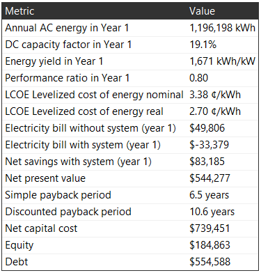
Case – I gives detail analysis of SET-A agriculture farms of locations Ganayigudem, Seetharampuram, Vegavaram and Ainavillilanka where as per the survey all these locations of SET-A share a load of 647kW, so a solar plant of capacity 650kW has been constructed in SAM software to analyze for SET-A agriculture farms, for economic development of farmers community. For this analysis the weather conditions data is required for locations Ganayigudem latitude 16.7761° N and longitude 81.1458° E, Seetharampuram latitude 16.7519° N and longitude 81.4289° E, Vegavaram latitude 16.7666° N and longitude 81.1212° E and Ainavillilanka latitude 16.6772° N and longitude 82.0203° E with the help of this latitude and longitude in SAM nrel website weather data files are available from nrel website these files to be downloaded and add them in SAM software location and resource file so the particular weather file will be added now by clicking on download and add to library the file will be upload for access weather data. For set-A as shown in Figure 6 the cumulative data was shown contains annual AC energy in year 1, DC capacity factor in year 1, LOCE are 3.38 \$/kWh and 2.7 \$/kWh, net present value 544.277\$, simple payback period 6.5 years and discounted payback period 10.6 years.
Figure 6. Cumulative data for set-A
Figure 7 shows monthly AC energy for year 1 starting from January to December and the values are January-116062 kWh, Febuary-115940 kWh, March-121849 kWh, April-110498 kWh, May-108740 kWh, June-73048.3 kWh, July-66990.9 kWh, August-76757.8 kWh, September-85526.4 kWh, October-108030 kWh, November-101032 kWh and December-111724kWh. All these monthly AC energies generated was obtain for set-A was due to the weather data uploaded in SAM software. The annual energy was 1196198 kWh. Figure 8 shows annual AC energy for year on hourly basis. The annual energy was total energy generated for year one.
Figure 7. Monthly AC energy
Figure 8. Annual AC energy
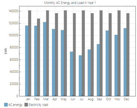
Figure 9 shows monthly AC energy and load profiles for year 1 starting from January to December and the values are January-141050 kWh, Febuary-127400 kWh, March-141050 kWh, April-136500 kWh, May-141050 kWh, June-136500 kWh, July-141050 kWh, August-136500 kWh, September-141050 kWh, October-136500 kWh, November-141050 kWh and December-136500 kWh. These load profiles show the loads applied to set-A with the help of data collected from farmers i.e., actual load required.
Figure 9. Monthly AC energy and load
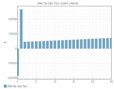
Figure 10. After tax cash flow-system lifetime for 25 years
Figure 10 shows after tax cash flow-system lifetime for 25 years and the values for year one 267007\$, two 46239.8\$, three 47315\$, four 48396.7\$, five 49484.6\$, six 50578\$, seven 51676.9\$, eight 52780.7\$, nine 53889\$, ten 55001.4\$, eleven 56117.4\$, twelve 57236.2\$, thirteen 58357.5\$, fourteen 59480\$, fifteen 60604.7\$, sixteen 61729.3\$, seventeen 62909.6\$, eighteen 64092.3\$, nineteen 65276.1\$, twenty 66460.1\$, twenty one 67643.7\$, twenty two 68825.9\$, twenty three 70006.6\$, twenty four 71183.8\$, twenty five 72357.1\$ where the x-axis shows number of years and Y-axis shows value in dollars. Here from Figure 10 shows the returns of revenue i.e., in the starting the returns are low due to initial costs, after that year to year the returns are increasing. Figure 11 shows electricity net generation for 25 years and the values for year one 1.1962e+06 kWh, two 1.19015e+06 kWh, three 1.18411e+06 kWh, four 1.17806e+06 kWh, five 1.17202 e+06 kWh, six 1.16597e+06 kWh, seven 1.15992e+06 kWh, eight 1.15387e+06 kWh, nine 1.141783e+06 kWh, ten 1.1478e+06 kWh, eleven 1.13573e+06 kWh, twelve 1.12968e+06 kWh, thirteen 1.12363e+06 kWh, fourteen 1.11758e+06 kWh, fifteen 1.11153e+06 kWh, sixteen 1.10548e+06 kWh, seventeen 1.09943e+06 kWh, eighteen 1.09339e+06 kWh, nineteen 1.08734e+06 kWh, twenty 1.08129e+06 kWh, twenty one 1.07524e+06 kWh, twenty two 1.06919e+06 kWh, twenty three 1.06314e+06 kWh, twenty four 1.05709e+06 kWh, twenty five 1.05104e+06 kWh. In Figure 11 it is shown a slight change in net generation due to depreciation percentage of plant.
Figure 11. Electricity net generation for 25 years
Figure 12. System power generated profile for all months
Figure 12 shows data of system power generated for all months from January to February, along with this annual report was also given where the x-axis shows number of days in a month and Y-axis shows number of days in a year.
3.2 SET-B agriculture farms
Case – II gives detail analysis of SET-B agriculture farms of locations Jogannapalem, Naguladevupadu and Veeravallipalem where as per the survey all these locations of SET-B share a load of 259kW, so a solar plant of capacity 300kW has been constructed in SAM software to analyze for SET-B agriculture farms for economic development of farmers community. For this analysis the weather conditions data is required for locations Jogannapalem latitude 16.8150° N and longitude 81.1679° E, Naguladevupadu latitude 16.8319° N and longitude 81.1874° E and Veeravallipalem latitude 16.6882°N and longitude 82.0012° E with the help of this latitude and longitude in SAM nrel website weather data files are available from nrel website these files to be downloaded and add them in SAM software location and resource file so the particular weather file will be added now by clicking on download and add to library the file will be upload for access weather data. For set-A as shown in Figure 13 the cumulative data was shown contains annual AC energy in year 1, DC capacity factor in year 1, LOCE are 3.18 \$/kWh and 2.54 \$/kWh, net present value 289.640\$, simple payback period 5.9 years and discounted payback period 9.1 years.
Figure 13. Cumulative data for set-B
Figure 14. Monthly AC energy
Figure 14 shows monthly AC energy for year 1 starting from January to December and the values are January-54,898.9 kWh, Febuary-54,143.8 kWh, March-57,777.1 kWh, April-54,630.3 kWh, May-47,480.6 kWh, June-40,637.4 kWh, July-37,701.2 kWh, August-41,374.3 kWh, September-42,019.3 kWh, October-50,459.8 kWh, November-51,454.8 kWh and December-52,853 kWh. The annual energy was 585,431 kWh. All these monthly AC energies generated was obtain for set-B was due to the weather data uploaded in SAM software. Figure 15 shows annual AC energy for year on hourly basis. The annual energy was total energy generated for year one.
Figure 15. Annual AC energy
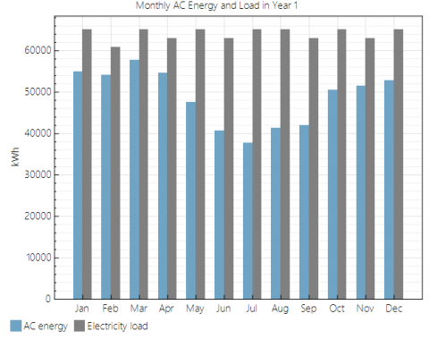
Figure 16. Monthly AC energy and load
Figure 16 shows monthly AC energy and load profiles for year 1 starting from January to December and the values are January-65100 kWh, Febuary-60900 kWh, March-65100 kWh, April-63000 kWh, May-65100 kWh, June-63000 kWh, July-65100 kWh, August-65100 kWh, September-63000 kWh, October-65100 kWh, November-63000 kWh and December-65100 kWh. These load profiles show the loads applied to set-B with the help of data collected from farmers i.e., actual load required.
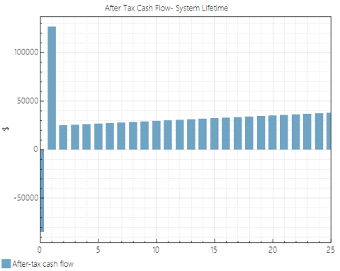
Figure 17. After tax cash flow-system lifetime for 25 years
Figure 17 shows after tax cash flow-system lifetime for 25 years and the values for year one 100741\$, two 20238.7\$, three 20386.2\$, four 20538.3\$, five 20695.3\$, six 20857.2\$, seven 21024.2\$, eight 21196.5\$, nine 21374.2\$, ten 21557.6\$, eleven 21746.9\$, twelve 21942.1\$, thirteen 22143.6\$, fourteen 22351.5\$, fifteen 22566.1\$, sixteen 22787.6\$, seventeen 23016.2\$, eighteen 23252.1\$, nineteen 23495.7\$, twenty 23747.1\$, twenty one 24006.6\$, twenty two 24274.6\$, twenty three 24551.2\$, twenty four 24836.9\$, twenty five 25131.8\$.
Figure 18. Electricity net generation for 25 years
Here from Figure 17 user can see the returns of revenue i.e., in the starting the returns are low due to initial costs, after that year to year the returns are increasing. Figure 18 shows electricity net generation for 25 years and the values for year one 585431 kWh, two 582474 kWh, three 579518 kWh, four 576561 kWh, five 573604 kWh, six 570648 kWh, seven 567692 kWh, eight 564735 kWh, nine 561778 kWh, ten 558821 kWh, eleven 555864 kWh, twelve 552907 kWh, thirteen 549949 kWh, fourteen 546991 kWh, fifteen 544032 kWh, sixteen 541074 kWh, seventeen 538115 kWh, eighteen 535157 kWh, nineteen 532199 kWh, twenty 529240 kWh, twenty one 526282 kWh, twenty two 523323 kWh, twenty three 520364 kWh, twenty four 517406 kWh, twenty five 514447 kWh. In Figure 18 user can see a slight change in net generation due to depreciation percentage of plant.
Figure 19 shows data of system power generated for all months from January to February along with this annual report was also given where the x-axis shows number of days in a month and Y-axis shows number of days in a year.
Figure 19. System power generated
3.3 SET-C agriculture farms
Case – III gives detail analysis of SET-C agriculture farms of locations Manduru where as per the survey all these locations of SET-C share a load of 398kW, so a solar plant of capacity 400kW has been constructed in SAM software to analyze for SET-C agriculture farms for economic development of farmers community. For this analysis the weather conditions data is required for locations Manduru latitude 16.1640° N and longitude 80.6375° E with the help of this latitude and longitude in SAM nrel website weather data files are available from nrel website these files to be downloaded and add them in SAM software location and resource file so the particular weather file will be added now by clicking on download and add to library the file will be upload for access weather data. For set-A as shown in Figure 20 the cumulative data was shown contains annual AC energy in year 1, DC capacity factor in year 1, LOCE are 3.33 \$/kWh and 2.66 \$/kWh, net present value 333,167\$, simple payback period 6.5 years and discounted payback period 10.5 years.
Figure 20. Cumulative data for set-C
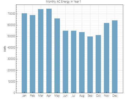
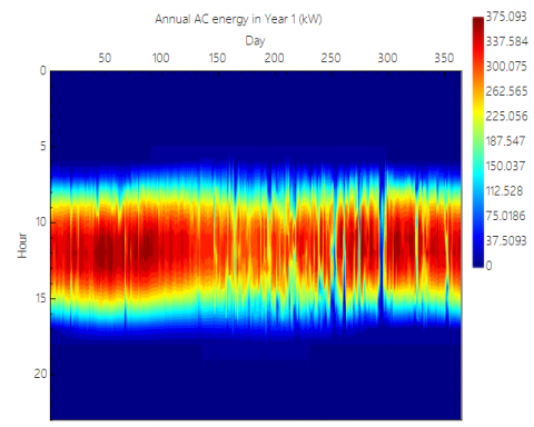
Figure 21 shows monthly AC energy for year 1 starting from January to December and the values are January-70433.3 kWh, Febuary-68910.2 kWh, March-74040.7 kWh, April-74399.8 kWh, May-65926.9 kWh, June-55040 kWh, July-55020.2 kWh, August-53791.2 kWh, September-49954.6 kWh, October-51240.6 kWh, November-61829.3 kWh and December-64153.3 kWh. The annual energy was 744740 kWh. All these monthly AC energies generated was obtain for set-C was due to the weather data uploaded in SAM software. Figure 22 shows annual AC energy for year on hourly basis. The annual energy was total energy generated for year one.
Figure 21. Monthly AC energy
Figure 22. Annual AC energy in year
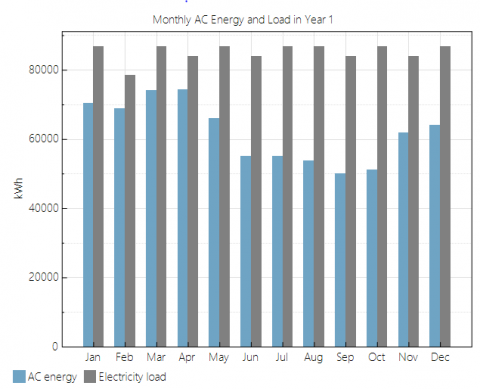
Figure 23 shows monthly AC energy and load profiles for year 1 starting from January to December and the values are January-86800 kWh, Febuary-78400 kWh, March-86800 kWh, April-84000 kWh, May-86800 kWh, June-84000 kWh, July-86800 kWh, August-86800 kWh, September-84000 kWh, October-86800 kWh, November-84000 kWh and December-86800 kWh. These load profiles show the loads applied to set-C with the help of data collected from farmers i.e., actual load required.
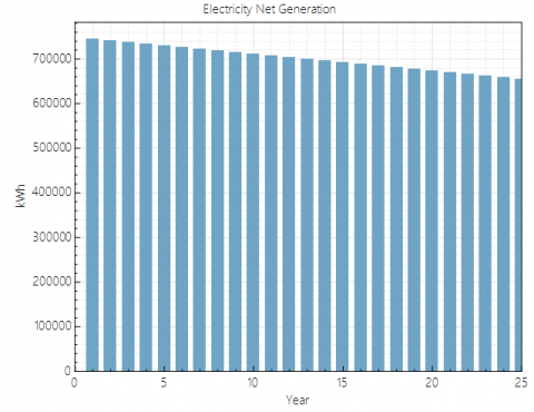
Figure 24 shows after tax cash flow-system lifetime for 25 years and the values for year one 164014\$, two 28728.1\$, three 29343.7\$, four 29960.9\$, five 30579.5\$, six 31199.1\$, seven 31819.6\$, eight 32440.1\$, nine 33060.6\$, ten 33680.7\$, eleven 34299.8\$, twelve 34917.4\$, thirteen 35533.4\$, fourteen 36146.8\$, fifteen 36757.2\$, sixteen 37364.4\$, seventeen 37967.4\$, eighteen 38565.7\$, nineteen 39158.9\$, twenty 39746\$, twenty one 40338.6\$, twenty two 40952.6\$, twenty three 41560.3\$, twenty four 42161.4\$, twenty five 42754.8\$. Here from Figure 24 user can see the returns of revenue i.e., in the starting the returns are low due to initial costs, after that year to year the returns are increasing. Figure 25 shows electricity net generation for 25 years and the values for year one 744740 kWh, two 740975 kWh, three 737210 kWh, four 733444 kWh, five 729679 kWh, six 725913 kWh, seven 722149 kWh, eight 718383 kWh, nine 714617 kWh, ten 710852 kWh, eleven 707086 kWh, twelve 703321 kWh, thirteen 699556 kWh, fourteen 695790 kWh, fifteen 692024 kWh, sixteen 688259 kWh, seventeen 684493 kWh, eighteen 680727 kWh, nineteen 676961 kWh, twenty 673195 kWh, twenty one 669430 kWh, twenty two 665664 kWh, twenty three 661898 kWh, twenty four 658132 kWh, twenty five 654366 kWh. In Figure 25 user can see a slight change in net generation due to depreciation percentage of plant.
Figure 23. Monthly AC energy and load
Figure 24. After tax cash flow-system lifetime for 25 years
Figure 25. Electricity net generation for 25 years
Figure 26. System power generated profile for all months
Figure 26 shows data of system power generated for all months from January to February along with this annual report was also given where the x-axis shows number of days in a month and Y-axis shows number of days in a year.
Energy generation for all the three clusters for twenty-five years are shown in Figure 27, where the red indicates for set-B and green indicates set-C and blue indicates set-A. The monthly generation profiles for all the twelve months for each case i.e., for sets- A, B & C are given in Figure 28.
Figure 27. Electricity net Generation for 25 years for all three sets i.e. A, B & C
Figure 28. Monthly Generation for 12 months for all three sets i.e. A, B & C
To address the objectives of designing the PV systems from these, SAM software simulation results it is found that with and without PV system revenue savings. And with the help of actual solar power selling prices including government norms and incentives all the three plants are getting a good payback period. Limitations and uncertainties that could affect this work are as these climate changes are uncertain now-a-days there will be slight changes in getting output in practical way. By updating the weather data and by reconsidering the selling prices of power the PV plant stability can be maintained.
The escalating demand for electricity in agricultural applications across India necessitates the exploration of individual photovoltaic (PV) systems. To accommodate this electrical load, empirical data from farmers was gathered to guide the installation of a PV plant. This necessitated a comprehensive techno-economic analysis, conducted using the System Advisor Model (SAM) software. The installation of solar plants, as demonstrated via SAM, encompasses a financial model, carbon emission reductions, and aligns with the economic and environmental objectives of the Government of India.
For eight distinct locations in Andhra Pradesh, India, a survey of the electrical load connected to the agricultural grid suggested the installation of solar plants in three sets - A, B, and C - with capacities of 650kW, 300kW, and 400kW respectively. The analysis, which considered both financial and non-financial factors, indicated that these plants should be grid-connected given India's near-complete electrification. This allows users to utilize the energy required by agricultural farms in instances of insufficient solar plant generation, thereby reducing energy storage costs. The primary objective was to provide a practical overview of a solar plant for agricultural farms using the SAM software.
The key outcomes of the PV systems for Set-A, B, and C were as follows: Set-A had a levelized cost of energy of 2.7 \$/kWh, which was economical, and net savings with the system for one year was \$83,185. For Set-B, the levelized cost of energy was 2.54 \$/kWh, and the net savings amounted to \$41,992. Set-C had a levelized cost of energy of 2.66 \$/kWh, with net savings of \$51,402. The analysis determined the payback periods of these three sets to be 6.5 years, 5.9 years, and 6.5 years respectively, which aligns with the practical return period range of 5 to 10 years.
The feasibility and benefits of PV systems for powering agricultural loads were assessed using the Solar Energy Corporation of India (SECI), where the Indian Government solicits tenders for solar plant installation. By considering these practical costs, load rates were established for practical analysis, yielding tangible results. The installation of these PV plants resulted in CO2 emissions reductions of about 714.48 metric tons for Set-A, 306.2 metric tons for Set-B, and 408.27 metric tons for Set-C.
This study was not without limitations. Uncertainties in climate changes may cause slight deviations in practical output. However, given India's high degree of electrification, storage systems are not necessary, reducing initial and maintenance costs. Additionally, excess energy can be sold to the grid, generating income and promoting the use of solar energy in agriculture.
The future scope of this work encompasses the installation of microgrids for village communities, reinforcing the role of solar plants in agricultural farms. This research provides an essential foundation for understanding the design, installation, and benefits of solar plants in agricultural settings.
[1] System advisor model. https://sam.nrel.gov/.
[2] Aziz, Y., Janjua, A.K., Hassan, M., Anwar, M., Kanwal, S., Yousif, M. (2023). Techno-economic analysis of PV systems installed by using innovative strategies for smart sustainable agriculture farms. Environment, Development and Sustainability, 1-22. https://doi.org/10.1007/s10668-023-02919-5
[3] Ghodusinejad, M.H., Ghodrati, A., Zahedi, R., Yousefi, H. (2022). Multi-criteria modeling and assessment of PV system performance in different climate areas of Iran. Sustainable Energy Technologies and Assessments, 53: 102520. https://doi.org/10.1016/j.seta.2022.102520
[4] Chaianong, A., Bangviwat, A., Menke, C., Breitschopf, B., Eichhammer, W. (2020). Customer economics of residential PV–battery systems in Thailand. Renewable Energy, 146: 297-308. https://doi.org/10.1016/j.renene.2019.06.159
[5] Alharthi, Y.Z., AlAhmed, A., Ibliha, M., Chaudhry, G.M., Siddiki, M.K. (2016). Design, simulation and financial analysis of a fixed array commercial PV system in the City of Abu Dhabi-UAE. In 2016 IEEE 43rd Photovoltaic Specialists Conference (PVSC), pp. 3292-3295. https://doi.org/10.1109/PVSC.2016.7750274
[6] Mahima, Karakoti., I., Pathak., P.P., Nandan, H. (2018). A comprehensive study of ground measurement and satellite derived data of global and diffuse radiation. Environmental Progress & Sustainable Energy, 38(3): e13060. https://doi.org/10.1002/ep.13060
[7] Pimentel da Silva, G.D. (2017). Utilization of the system advisory model to estimate electricity generation by grid connected photovoltaic projects in all regions of Brazil. International Journal of Software Engineering and Its Application, 11(7): 1-12. https://doi.org/10.14257/ijseia.2017.11.7.01
[8] Alhendal, Y., Touzani, S. (2023). Influence of inclination angles on convective heat transfer in solar panels. International Journal of Heat and Technology, 41(4): 808-814. https://doi.org/10.18280/ijht.410403
[9] Santos, E.C., Macêdo, E.N., Magno, R.N.O., Galhardo, M.A.B., Oliveira, L.G.M., Brito, A.U., Macêdo, W.N. (2023). Exergetic assessment and computational modeling of a solar-powered directly-coupled air conditioning system: An application in library cooling. International Journal of Heat and Technology, 41(4): 854-868. https://doi.org/10.18280/ijht.410408
[10] Alshare, A., Tashtoush, B., Altarazi, S., El-Khalil, H. (2020). Energy and economic analysis of a 5 MW photovoltaic system in northern Jordan. Case Studies in Thermal Engineering, 21: 100722. https://doi.org/10.1016/j.csite.2020.100722
[11] Imam, A.A., Al-Turki, Y.A. (2019). Techno-economic feasibility assessment of grid-connected PV systems for residential buildings in Saudi Arabia—A case study. Sustainability, 12(1): 262. https://doi.org/10.1016/j.seta.2013.06.002
[12] Xiong, L., Nour, M. (2019). Techno-economic analysis of a residential PV-storage model in a distribution network. Energies, 12(16): 3062. https://doi.org/10.3390/en12163062
[13] Shivakumar, A., Kruitwagen, L., Weinstein, M., Spiteri, S., Arderne, C., Almulla, Y., Usher, W., Howells, M., Hawkes, A. (2021). A techno-economic and financial analysis of a Gulf-India undersea electricity interconnector. https://doi.org/10.21203/rs.3.rs-690329/v1
[14] da Silva, G.D.P. (2017). Utilisation of the System Advisor Model to estimate electricity generation by grid-connected photovoltaic projects in all regions of Brazil. International Journal of Software Engineering and Its Applications, 11(7): 1-12. https://doi.org/10.14257/ijseia.2017.11.7.01
[15] New & Renewable Energy Development Corporation of Andhra Pradesh Ltd. https://www.nredcap.in/Default.aspx.
[16] Solar Energy Corporation of India (SECI) - https://www.seci.co.in/.
[17] Agostini, A., Colauzzi, M., Amaducci, S. (2021). Innovative agrivoltaic systems to produce sustainable energy: An economic and environmental assessment. Applied Energy, 281: 116102. https://doi.org/10.1016/j.apenergy.2020.116102