Nurlan Temirbekov![]() | Yerzhan Malgazhdarov
| Yerzhan Malgazhdarov![]() | Dinara Tamabay*
| Dinara Tamabay*![]() | Almas Temirbekov
| Almas Temirbekov![]()
© 2023 IIETA. This article is published by IIETA and is licensed under the CC BY 4.0 license (http://creativecommons.org/licenses/by/4.0/).
OPEN ACCESS
In this study, the dispersal of atmospheric pollutants from point sources and their photochemical transformations are examined. The mass conservation principle underlies a system of differential equations formulated to describe the transfer and transformation processes, incorporating stoichiometric formulas and reaction rate constants. The atmospheric boundary layer model and the transport-transformation equation of pollutants are considered, integrating a specific parameter to assess the influence of anthropogenic heat sources and surface heterogeneity on pollutant dispersion. Using Ust-Kamenogorsk, an industrial city in Kazakhstan, as a case study, the model accounts for variations in photochemical transformations due to weather conditions, ambient temperature, and time of day. To facilitate numerical simulations of atmospheric pollution and visualize various scenarios, a software application package was created, incorporating photochemical transformations. The developed suite of applications has been verified with real data and benchmarked against contemporary software packages such as WRF and SILAM. Moving forward, the refined model aims to forecast air pollution patterns in industrial cities across Kazakhstan.
atmospheric boundary layer equation, transformation of harmful substances, mathematical modeling, differential equation, difference scheme, stability, computational algorithm, numerical experiment
Atmospheric air pollution continues to pose a significant challenge in numerous cities across the Republic of Kazakhstan. Predominant sources of these pollutants comprise enterprises within thermal power engineering, ferrous and non-ferrous metallurgy, and oil production and refining sectors, alongside road and rail transport.
Rapid socio-economic development, consistent population growth, the absence of best available technologies (BAT) in industrial enterprises and thermal power plants, and underdeveloped public transport infrastructure have collectively escalated air pollution levels in the Republic's industrial cities.
Globally, it is estimated that seven million premature deaths annually are attributable to indoor air pollution, surpassing the combined mortality rates of high-fatality diseases such as malaria, tuberculosis, and AIDS.
The gravity of atmospheric pollution and the necessity to study air quality were underscored following the London smog event in 1952, which precipitated thousands of premature deaths [1]. China, currently the leading nation with densely populated cities and a developed industrial sector, has established over 370,000 new industrial enterprises in the past four decades. Gautam et al. [2] examined air pollution, specifically PM2.5, in 21 Chinese cities, while Kuerban et al. [3], Liu et al. [4], Chang et al. [5, 6] assessed carbon-containing aerosols in Shanghai. Their findings underscored the heavy pollution in China's eastern, northern, and northeastern cities, regions with a high concentration of industrial facilities.
Existing research on air quality in industrial cities, both international and domestic, has highlighted an information deficit concerning atmospheric pollution, emphasizing the need for comprehensive studies [7, 8]. One such study [7] evaluated additional morbidity and mortality across 21 cities in Kazakhstan due to fine particle exposure. The study estimated that air pollution contributes to 8,134 premature adult deaths annually, with significant variations among cities. However, due to the inadequate network of fine particle monitoring posts, the study relied on data concerning total suspended particles. The authors recommended recalculating health impacts based on measured PM2.5 concentrations in city atmospheres following the expansion of the monitoring network [7].
The investigation conducted by Kerimray et al. [8] sought to gauge the influence of COVID-19 quarantine measures, implemented in 2020, on the concentration of atmospheric pollutants in Almaty. The authors juxtaposed daily pollutant concentrations across distinct phases: pre-quarantine, during quarantine, and post-quarantine. The findings indicated a marked reduction in pollution levels during the quarantine period.
Regrettably, the issue of air pollution persists across all regions of Kazakhstan. In contrast, numerous European countries, the USA, Canada, and Japan have all witnessed a significant decrease in emissions and pollutant concentrations, primarily due to the strict policy guidelines and regulatory rules enforced, coupled with the establishment of regular monitoring systems [9].
Historically, due to its socio-economic development, the East Kazakhstan region has emerged as one of the nation's most ecologically disadvantaged areas. Ust-Kamenogorsk, a highly urbanized city within this region, houses a plethora of industrial enterprises spanning diverse technological sectors. These include non-ferrous metallurgy, nuclear industrial and rare metal complexes, thermal power engineering, transport, as well as the food industry and utilities. This industrial density exacerbates the city's pollution, further compounded by emissions from transport and the private sector. The city's air is typically laden with pollutants such as sulfur dioxide, nitrogen dioxide, carbon monoxide, phenol, formaldehyde, chlorine, inorganic arsenic compounds, hydrogen chloride, hydrogen fluoride, sulfuric acid, hydrogen sulfide, ammonia, benz(a)pyrene, and six metallic elements: lead, zinc, copper, cadmium, beryllium, and mercury [10].
Air pollution in Ust-Kamenogorsk is influenced by an array of sources and is further aggravated by the unique atmospheric circulation dictated by its geographical location. The city is situated in a river valley surrounded by mountains, a topography that gives rise to stagnant and mountain-valley winds, leading to unfavorable meteorological conditions such as temperature inversions, calm surface layers, fogs, and unfavorable wind directions. These adverse conditions trigger chemical transformations in pollutants. The convergence of windless conditions with fogs and inversions contributes to peak pollution levels. Approximately 85% of fog occurrences coincide with periods of windless weather, while the remaining 15% occur when the wind speed varies between 1-3 m/s [10].
Numerous scientific publications worldwide, including in Kazakhstan, have focused on the topic of atmospheric pollutant dispersion, exploring various methods for modeling this process. The works of Marchuk [11], Penenko et al. [12], Aloyan et al. [13], Baklanov et al. [14], and Newstadt and Van Dope [15], Nieuwstadt [16] have been instrumental in advancing mathematical models for atmospheric pollution.
The development of an information system employing a probabilistic-statistical approach for simulating the transfer of vehicular emissions into the atmosphere was demonstrated instudies [17, 18].
Artificial neural networks have proven their efficacy as accurate predictors for classification and regression tasks, as illustrated by the literature. They have been utilized for predicting the surface boundary layer of the atmosphere, air pollution indicators, and simulating the effects of point sources. Worldwide, platforms for air monitoring leveraging artificial intelligence and the Internet of Things (IoT) are under development [19-22].
In the study [19], a multiple regression model was established using machine learning algorithms to discern the relationship between bioexperiment data and pollutant data derived from chemical analytical studies in Almaty, Kazakhstan, thereby gauging the impact of atmospheric pollution on the environment.
The prediction and detection of PM10 concentrations have been prioritized due to their detrimental effects on human health. Machine learning (ML) approaches offer enhanced precision for predicting and classifying future PM10 concentrations [21]. Accordingly, in the study [20], three distinct ML algorithms were employed: a decision tree, an accelerated regression tree, and a random forest.
In the study [22], a typical dusty weather case was selected for analysis in the northeast of the Tibetan Plateau, following which six ML methods and a time series regression model were applied to predict PM10 concentration in the area.
Machine learning methods are optimally utilized in tasks that lack a stringent mathematical model, as a system trained solely on available expert assessments can emulate a pattern that is otherwise challenging and nearly impossible to formalize.
Despite the existing body of work studying the atmospheric air of Kazakhstan's industrial cities, the issue warrants further detailed investigation.
In this article, the problem of scattering impurities from specific point sources is explored, meticulously considering the influence of weather conditions and time of day on the photochemical transformation of these impurities. The aim is to comprehend how these factors dictate the dispersion and subsequent transformation of harmful impurities. To elucidate this, the results of extensive numerical simulations are presented. This study specifically investigates the dynamics of impurity dispersion and transformation, considering the prevailing mesometeorological processes in the city of Ust-Kamenogorsk. The objective is to understand the intricate relationship between impurity dispersion, photochemical reactions, and local meteorological conditions within this city's context.
A suite of application programs has been developed, rigorously validated using actual data, and subsequently benchmarked against contemporary WRF and SILAM software packages within the context of industrial cities in Kazakhstan. This model is intended to be employed for forecasting air quality in industrial urban areas in the future.
2.1 Conversion of harmful impurities: A chemical modeling approach
Studies of the composition of atmospheric air in conditions of variable weather conditions and a diverse territory require the use of models based on the physico-chemical characteristics of substances. These models make it possible to visually establish cause-and-effect relationships and use extensive amounts of data on terrain and atmospheric conditions.
For effective modeling of chemical reactions in the atmosphere, a complex of mechanisms operating on a computer has been developed. Each of them takes into account a certain set of substances. Among the main mechanisms for modeling chemical processes in the atmosphere, CB4, RADM2, RACM, SAPRC-97, EMEP, KOREM and others can be distinguished [23].
For a more detailed study of the composition of atmospheric air on the territory of a certain region, it is reasonable to use local models that are able to adequately take into account all the chemical mechanisms operating in this area.
In order to achieve accurate results in modeling the concentrations of pollutants in the industrial city of Ust-Kamenogorsk, a list of characteristic pollutants was compiled and their transformation scheme by chemical reactions was developed. Differential equations using stoichiometric formulas and reaction rate constants take into account the law of conservation of mass. To capture the changes that occur to harmful impurities during their transfer, the method introduced in studies [10, 24] is employed. This approach utilizes the most prevalent types of harmful substances, including CH2O, CO, CO2, SO2, SO3, HSO3, NO, NO2, NO3, HNO3, MgO, CaO, H2SO4, MgSO2, CaSO2, and their chemical reactions, to simulate photochemical processes.
As an illustration, when SO2 molecules absorb solar radiation, they become energized and undergo a reaction with oxygen in an excited state, resulting in the formation of SO3 and O3:
$\begin{gathered}\mathrm{SO}_2+h v \rightarrow \mathrm{SO}_2{ }^* \\ \mathrm{SO}_2{ }^*+\mathrm{O}_2 \rightarrow \mathrm{SO}_3+\mathrm{O}\end{gathered}$
Thick smog appears in the city of Ust-Kamenogorsk during adverse weather conditions (AWC).
In nature, there are two distinct types of smog: London type, which is reducing, and Los Angeles type, which is photochemical oxidative. Industrial cities tend to have restorative smog, which is a blend of smoke, soot, and sulfur dioxide. The highest levels of smog are typically observed in the early morning at around 0℃.
Consider the main types of smog: smog formation due to atmospheric pollution by soot or smoke containing sulfur dioxide SO2 and air pollution by car exhaust gases containing nitrogen oxides.
Sulfur oxidation proceeds in three states: gas, liquid, solid. SO2 molecules interacting with oxygen O2 in the atmosphere, forms sulfur trioxide SO3 and three oxygen O3:
$\mathrm{SO}_2{ }^*+\mathrm{O}_3 \rightarrow \mathrm{SO}_3+\mathrm{O}_2$
or interacting with carbon monoxide CO forms sulfur oxide SO and carbon dioxide CO2.
$\mathrm{SO}_2{ }^*+\mathrm{CO} \rightarrow \mathrm{SO}+\mathrm{CO}_2$
or by reaction involving the third body M:
$\mathrm{SO}_2{ }^*+\mathrm{M} \rightarrow \mathrm{SO}+\mathrm{M}$
The second type of smog, known as photochemical smog, requires photochemical reactions to occur, which lead to the formation of ozone (O3). This reaction is triggered by the presence of hydrocarbons and nitrogen oxides. The concentration of O3 in the air samples begins to increase when the ratio of NO2 and NO concentrations is at its maximum. The formation of O3 in the presence of nitrogen oxides is initiated by solar radiation with a wavelength of less than 580 nm, and it is more intense in air containing NO2. Solar radiation with wavelengths ranging from 285 nm to 580 nm can reach the Earth's surface.
The chemical transformations are described by a system of fifteen differential equations [11]. Some equations, for example, for CH2O, CO, CO2 the equations have the following form:
$\frac{d \varphi_{\mathrm{CH}_2 \mathrm{O}}}{d t}=-k_{60} \varphi_{\mathrm{CH}_2 \mathrm{O}}-k_{62} \varphi_{\mathrm{CH}_2 \mathrm{O}}+f_{\mathrm{CH}_2 \mathrm{O}}$ (1)
$\frac{d \varphi_{C O}}{d t}=k_{60} \varphi_{C H_2 O}-k_{65} \varphi_{C O}-k_{141} \varphi_{C O}+f_{C O}$ (2)
$\frac{d \varphi_{C O_2}}{d t}=k_{65} \varphi_{C O}-k_{141} \varphi_{C O}+f_{C O_2}$ (3)
For other chemicals the corresponding reactions are also selected.
Unlike the work [11], this research takes into account the $\gamma_i(p)$ parameter, which is determined depending on weather conditions and time of day, i is the number of the corresponding reaction. In order to uphold the principle of mass conservation, differential Eqs. in the form of (1)-(3) were formulated. These equations consider the transfer of substance fractions, where a fraction is subtracted from its original substance and added to the volume of the newly formed substance during a reaction.
In the equations of chemical kinetics, the coefficients k60, k62 and others, called the rate constants of chemical reactions, are known in advance [11].
2.2 Mathematical model of the boundary layer of the atmosphere
In order to examine the impact of anthropogenic heat sources, detrimental substances, and surface heterogeneity on the atmosphere of an industrial city, a three-dimensional domain $\Omega$ is utilized, following a model of the atmospheric boundary layer. The model is based on previous studies [10-12].
Equations of motions and continuity equation:
$\begin{gathered}\frac{\partial u_i}{\partial t}+\frac{\partial u_i u_j}{\partial x_j}=-\frac{\partial p}{\partial x_i}+a_i K_i+\frac{\partial}{\partial x_3}\left(v \frac{\partial u_i}{\partial x_3}\right)+\Delta u_i \\ \frac{\partial u_j}{\partial x_j}=0, i=1,2,3\end{gathered}$ (4)
where, $u=\left(u_1, u_2, u_3\right)$ is a velocity vector, $p=\left(p_1, p_2, p_3\right)$ is pressure, $x=\left(x_1, x_2, x_3\right)$ is Cartesian coordinates, $a=(1,-1, \lambda), K=\left(u_1, u_2, \theta\right), t$ is time, in the second term in the left part and in the continuity equation summation is performed by repeating indices $j(j=1,2,3)$. Heat inflow equation:
$\frac{\partial \theta}{\partial t}+\frac{\partial u_i \theta}{\partial x_i}+S u_3=\frac{\partial}{\partial x_3}\left(v \frac{\partial \theta}{\partial x_3}\right)+\Delta \theta$ (5)
here, $\theta$ is background potential temperature, ν is vertical coefficient of turbulent exchange, S is stratification parameter. Equation of transfer of harmful substances in the atmosphere:
$\begin{gathered}\frac{\partial \varphi_q}{\partial t}+u_j \frac{\partial \varphi_q}{\partial x_j}=\Delta \varphi_q+\frac{\partial}{\partial x_3}\left(v \frac{\partial \varphi_q}{\partial x_3}\right)+\alpha_q \varphi_q+\beta_q+ f_q, \sum_q \varphi_q=1\end{gathered}$ (6)
here, $\Delta=\frac{\partial}{\partial x_1} \mu_{x_1} \frac{\partial}{\partial x_1}+\frac{\partial}{\partial x_2} \mu_{x_2} \frac{\partial}{\partial x_2}$ is the differential operator of horizontal turbulent diffusion, $\lambda=\frac{g}{T}$ - convection parameter, $S=\frac{\partial \theta}{\partial x_3}$ is a stratification parameter, $g$-gravity acceleration, $T$-air temperature, $\mu_{x_1}, \mu_{x_2}$-coefficients of horizontal turbulence for motion and heat transfer, $v$-vertical coefficient of turbulent exchange for motion and heat transfer, $\theta$ is the background potential temperature, $l$ is the Coriolis parameter.
$\varphi_q$ is the fraction of the concentration of a harmful substance in the impurity, $f_q$ describes the sources of substances at the level of roughness, $\alpha_q, \beta_q$ are coefficients arising from the equations of transformations of impurities in the atmosphere, the index $q$ means the chemical formula of the substance. For example, for the fraction of concentrations of the substance $\mathrm{HSO}_3$ we have:
$\varphi_{\mathrm{HSO}_3}^{n+1}=\frac{\varphi_{\mathrm{HSO}_3}^{n+1 / 2}+\tau \beta_{\mathrm{HSO}_3}+\tau f_{\mathrm{HSO}_3}}{1-\tau \alpha_{\mathrm{HSO}_3}}$,
where, $\quad \alpha_{\mathrm{HSO}_3}=-\gamma_{154}(p) k_{154} \varphi_{\mathrm{HSO}_3} \quad$ and $\quad \beta_{\mathrm{HSO}_3}=$ $\gamma_{149}(p) k_{149} \varphi_{S O_2}, \gamma_i(p)$ is a parameter, that is determined depending on weather conditions and time of day.
In Eq. (5) and Eq. (6) as in Eq. (4), summation in the second term is performed by the index j.
The following initial and boundary conditions are given for the system of Eqs. (4)-(6):
$\begin{gathered}\vec{U}=\vec{U}^0\left(x_1, x_2, x_3\right), \theta=\theta^0\left(x_1, x_2, x_3\right), \varphi_q=\varphi_q^0\left(x_1, x_2, x_3\right) \\ \text { when } t=0 \\ u_1=u_{11}^{\prime}\left(x_2, x_3, t\right), u_2=u_{21}^{\prime}\left(x_2, x_3, t\right), u_3=0, \frac{\partial \theta}{\partial x_1}=0 \\ \varphi_q=\varphi_q^0 \text { when } x_1=0,0 \leq x_2 \leq Y \\ \frac{\partial u_1}{\partial x_1}=0, u_2=0, u_3=0, \frac{\partial \theta}{\partial x_1}=0, \frac{\partial \varphi_q}{\partial x_1}=0 \text { when } x_1=X \\ 0 \leq x_2 \leq Y\end{gathered}$
$\begin{gathered}u_1=u_{12}^{\prime}(x, z, t), u_2=u_{22}^{\prime}(x, z, t), u_3=0, \frac{\partial \theta}{\partial x_2}= \\ 0, \varphi_q=\varphi_q{ }^0 \text { when } x_2=0,0 \leq x_1 \leq X,\end{gathered}$ (7)
$\begin{gathered}
u_1=0, \frac{\partial u_2}{\partial x_2}=0, u_3=0, \frac{\partial \theta}{\partial x_2}=0, \frac{\partial \varphi_q}{\partial x_2}=0 \text { when } x_2=Y \\
0 \leq x_1 \leq X
\end{gathered}$
$u_1=0, u_2=0, u_3=0, \theta=0, p=0, \varphi_q=0$ when $x_3=H$,
$\begin{gathered}
u_3=0, h \frac{\partial u_1}{\partial x_3}=a_{u_1} u_1, h \frac{\partial u_2}{\partial x_3}=a_{u_1} u_2, h \frac{\partial \theta}{\partial x_3}=a_\theta\left(\theta-\theta_0\right), \\
\varphi_{q, 0}=\frac{f_q+a_\theta \varphi_{q, h} v}{\beta+a_\theta v_h} \text { when } x_3=h,
\end{gathered}$
here, $H$ is the atmospheric boundary layer height, $X, Y$-lateral boundaries of the region, $\varphi_{q, 0}, \varphi_{q, h}$-proportions of concentrations of matter $q$ at the level of roughness and the surface layer, $\theta_0$-roughness level temperature, $a_{u_1}=\frac{\psi_{u_1}\left(\varsigma_h\right)}{\eta_{u_1}\left(\varsigma_h, \varsigma_0\right)}$ -parameter resulting from the interaction between air flows and the underlying surface friction., $a_\theta=\frac{\psi_\theta\left(\varsigma_h\right)}{\eta_\theta\left(\varsigma_h, \varsigma_0\right)}$-a turbulent heat exchange parameter, $\beta$-a velocity-based value that characterizes the interaction between impurities and the underlying surface, $h$-surface layer height, $\varsigma_0, \varsigma_h$ dimensionless height parameters, $\psi_{u_1}, \psi_\theta$-Businger interpolation functions obtained using experimental data. A comprehensive overview of alternative interpolation formulas suggested by different authors can be found in studies [15, 16]. In our task, we utilized interpolation functions with the following form:
$\begin{gathered}\psi_{u_1}(\varsigma)=1+4.7 \varsigma, \psi_\theta(\varsigma)=0.74+4.7 \varsigma \text { when } \varsigma> \\ 0\end{gathered}$ (8)
$\eta_{u_1}\left(\varsigma, \varsigma_{u_1}\right)=\int_{\varsigma_{u_1}}^{\varsigma} \frac{\psi_{u_1}(\varsigma)}{\varsigma} d \varsigma, \eta_\theta\left(\varsigma, \varsigma_0\right)=\int_{\varsigma_0}^{\varsigma} \frac{\psi_\theta(\varsigma)}{\varsigma} d \varsigma$
Based on meteorological conditions, the boundary conditions of the type $u_1=u_{11}^{\prime}(y, z, t), u_2=u_{21}^{\prime}(y, z, t)$ are determined. The similarity theory of Monin-Obukhov and empirical functions from the study [11] were chosen for modeling the surface layer of the atmosphere at $x_3=h$. The terrain equation $x_3=\delta(x, y)$ is taken into account when setting boundary conditions for $\theta, \varphi_q$ in the surface layer at $x_3=h$. The remaining boundary conditions guarantee that perturbations are smooth and that the continuity equation holds at the boundary of the integrable domain.
The initial and boundary conditions (7) are selected from the most characteristic weather conditions of a particular city and vary depending on the time of year and the situation. The boundary conditions in the form of the first derivatives of the desired quantities are called “soft” boundary conditions and are placed at the output boundaries of the air flow.
The above-stated problems (4-7) are solved by the finite difference method and numerically performed by the splitting method for physical processes, which is successfully used in numerical solutions of the equations of aerohydrodynamics in natural variables.
The order of convergence and the order of accuracy of approximation of the system of differential equations under consideration are presented in studies [25, 26].
The numerical implementation algorithm is presented in study [13]. The above model and the developed algorithm were utilized to simulate atmospheric air pollution, taking into account photochemical transformations, at various input parameter values (Table 1). Numerical calculations were performed for an area of 35×35 kilometers and a fixed surface layer height of 3,500 meters. The stratification parameter S, which indicates temperature changes with height, was calculated using the vertical temperature gradient during the calculations.
Table 1. Input parameters for atmospheric air modeling taking into account photochemical transformations
|
Parameter Name |
Designation |
Value |
|
Convection parameter |
$\lambda$ |
$0.16 m(s \cdot \mathrm{deg})^{-1}$ |
|
Coriolis force |
$ l $ |
$ 10^{-4} \mathrm{~s}^{-1} $ |
|
Horizontal coefficient of turbulent exchange |
$ \mu_{\mathrm{x}_1} $ |
$ 6 \cdot 10^3 \mathrm{~m}^2 \mathrm{~s}^{-1} $ |
|
Vertical coefficient of turbulent exchange |
$ \mu_{x_2}$ |
$ 6 \cdot 10^3 \mathrm{~m}^2 \mathrm{~s}^{-1} $ |
|
Characteristic length scale |
$ L $ |
35000 m |
|
Wind |
$U^* $ |
$10 \mathrm{~m} \mathrm{~s}^{-1} $ |
|
Speed temperature |
$\theta^*$ |
20℃ |
Calculations were carried out on grids 100×100×50, 200×200×100 and 400×400×200. The numerical calculation was carried out on a modern personal computer with the following characteristics of Intel(R) Core(TM)i9-10900F CPU@2.80GHz, 32GB RAM. The results of numerical calculations are presented using the graphical editor Tecplot and Surfer.
To simulate the dispersion of harmful pollutants in the atmosphere, meteorological data were obtained from the regional branch of the Republican State Enterprise “Kazhydromet” in the East Kazakhstan region.
Data on concentrations of harmful substances were obtained from the monthly newsletter on the state of the environment of Kazhydromet [27].
When modeling the chemical transformation of harmful substances in the atmosphere [28], the following input data of the composition of harmful substances were taken (Table 2).
Table 2. Input parameters for atmospheric air modeling taking into account photochemical transformations
|
Reaction Number |
Amount of Harmful Substances (mg/hour) |
|
P1 |
CH2O=40 |
|
P2 |
CO=2 |
|
P3 |
CO2=2 |
|
P4 |
SO2=10 |
|
P5 |
SO3=10 |
|
P6 |
HSO3=2 |
|
P7 |
NO=10 |
|
P8 |
NO2=10 |
|
P9 |
NO3=2 |
|
P10 |
HNO3=2 |
|
P11 |
MgO=5 |
|
P12 |
CaO=5 |
|
P13 |
H2SO4=0 |
|
P14 |
MgSO4=0 |
|
P15 |
CaSO4=0 |
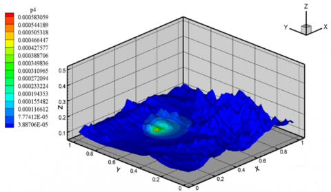
The calculation was carried out with a weak wind of the easterly direction of 1 m/s (Figures 1-3).
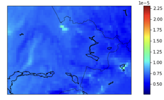
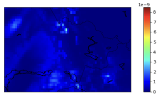
SILAM package that uses RSE Kazhydromet [29] (Figures 4-6), relies on a grid with a relatively large spatial step of 13km to simulate the spread of pollutants. In comparison, our developed software package, illustrated in Figures 1-3, uses a grid with a reduced spatial pitch from 350meters to 70meters. This allows us to achieve higher accuracy in modeling atmospheric processes, taking into account variables such as terrain and land use categories. This method provides a more accurate assessment of small-scale atmospheric processes in the study area.
Figure 1. Spread of amount of harmful substances CO
Figure 2. Spread of amount of harmful substances SO2
Figure 3. Spread of amount of harmful substances NO3
Figure 4. Spread of amount of harmful substances CO with the use of SILAM in the east Kazakhstan region
Figure 5. Spread of amount of harmful substances SO2 with the use of SILAM in the east Kazakhstan region
Figure 6. Spread of amount of harmful substances NO3 with the use of SILAM in the east Kazakhstan region
Calculations for the developed application software package and the SILAM package were made on meteorological data on April 7, 2023 at 06:00 am.
In examining atmospheric air pollution, a mathematical model has been developed which incorporates mesoscale atmospheric processes through a non-hydrostatic approximation. This model reflects the transfer and transformation of pollutants, terrain features, thermal variations in the underlying surface, weather conditions, and time of day.
A novel model has been constructed to represent the transformation of impurities within the atmospheric surface layer due to photochemical reactions, based on emissions data specific to industrial zones. The foundational mathematical model describing photochemistry has been augmented with new terms to account for emissions from the atmosphere in the form of droplets, fine particles, dust, and microparticles.
Chemical processes that differ during day and night were considered, and monitoring of atmospheric pollution and formation dynamics of harmful chemicals was conducted. It was observed that moderate wind speeds facilitated the assessment of water surfaces' and terrain orography's impact on pollutant dispersion. At high wind speeds, these factors were found not to induce significant deviations.
Previous studies employed a model of the atmospheric boundary layer to simulate atmospheric pollution, considering photochemical transformation. Systematic calculations have been performed in this study to validate the efficacy of this model. Real meteorological data and harmful substance emissions in industrial cities were analyzed in the present work. A suite of application programs was developed and validated using modern software packages WRF and SILAM for industrial cities in Kazakhstan.
These packages utilize a 13km grid, limiting the precision of modeling smaller processes and details of pollutant spread in cities due to computational resource constraints. The developed software suite enables the use of a more detailed grid, ranging from 350 to 70 meters. This allows for a more accurate consideration of land use characteristics and terrain, thus reflecting the actual atmospheric processes in the studied area.
Numerical experiments revealed that anthropogenic impurities released by industrial enterprises and carried by wind currents travel long distances depending on wind speed, leading to overlapping pollution fields. Under adverse weather conditions, anthropogenic admixture forms a cloud over an industrial city.
The developed software facilitates the assessment of an industrial city's air basin pollution. It considers the transformation of harmful substances, area orography, and provides a comprehensive pollution depiction at all nodal points using a database of pollution and meteorological data.
The developed application suite is utilized in the East Kazakhstan branch of RSE Kazhydromet to further refine hydrometeorological and environmental data issued by the WRF and SILAM programs. In this context, instead of the boundary conditions (7), values from the global calculation according to the aforementioned programs are used. Subsequently, the calculated area size can be reduced to the required grid step lengths. Thus, a computational experiment determines the optimal computational domain size for the city under study.
This research is funded by the Science Committee of the Ministry of Higher Education and Science of the Republic of Kazakhstan (Grant No.: BR18574148): Development of Geoinformation Systems and Monitoring of Environmental Objects.
[1] Hopke, P.K. (2010). The application of receptor modeling to air quality data. Pollution Atmosphérique, 91-109.
[2] Gautam, S., Patra, A.K., Kumar, P. (2019). Status and chemical characteristics of ambient PM2.5 pollutions in China: A review. Environment, Development and Sustainability, 21: 1649-1674. https://doi.org/10.1007/s10668-018-0123-1
[3] Kuerban, M., Waili, Y., Fan, F., Liu, Y., Qin, W., Dore, A.J., Peng, J.J., Xu, W., Zhang, F.S. (2020). Spatio-temporal patterns of air pollution in China from 2015 to 2018 and implications for health risks. Environmental Pollution, 258: 113659. https://doi.org/10.1016/j.envpol.2019.113659
[4] Liu, S.H., Zhu, C.Y., Tian, H.Z., Wang, Y.X., Zhang, K., Wu, B.B., Liu, X.Y., Hao, Y., Liu, W., Bai, X.X., Lin, S.M., Wu, Y.M., Shao, P.Y., Liu, H.J. (2019). Spatiotemporal variations of ambient concentrations of trace elements in a highly polluted region of China. Journal of Geophysical Research: Atmospheres, 124(7): 4186-4202. https://doi.org/10.1029/2018JD029562
[5] Chang, Y.H., Huang, K., Xie, M.J., Deng, C.R., Zou, Z., Liu, S.D., Zhang, Y.L. (2018). First long-term and near real-time measurement of trace elements in China’s urban atmosphere: temporal variability, source apportionment and precipitation effect. Atmospheric Chemistry and Physics, 18(16): 11793-11812. https://doi.org/10.5194/acp-18-11793-2018
[6] Chang, Y.H., Deng, C.R., Cao, F., Cao, C., Zou, Z., Liu, S.D., Lee, X.H., Li, J., Zhang, G., Zhang, Y.L. (2017). Assessment of carbonaceous aerosols in Shanghai, China-Part 1: Long-term evolution, seasonal variations, and meteorological effects. Atmospheric Chemistry and Physics, 17(16): 9945-9964. https://doi.org/10.5194/acp-17-9945-2017
[7] Kerimray, A., Assanov, D., Kenessov, B., Karaca, F. (2020). Trends and health impacts of major urban air pollutants in Kazakhstan. Journal of the Air & Waste Management Association, 70(11): 1148-1164. https://doi.org/10.1080/10962247.2020.1813837
[8] Kerimray, A., Baimatova, N., Ibragimova, O.P., Bukenov, B., Kenessov, B., Plotitsyn, P., Karaca, F. (2020). Assessing air quality changes in large cities during COVID-19 lockdowns: The impacts of traffic-free urban conditions in Almaty, Kazakhstan. Science of The Total Environment, 730: 139179. https://doi.org/10.1016/j.scitotenv.2020.139179
[9] Goshen, S., Novack, L., Erez, O., Yitshak-Sade, M., Kloog, I., Shtein, A., Shany, E. (2020). The effect of exposure to particulate matter during pregnancy on lower respiratory tract infection hospitalizations during first year of life. Environmental Health, 19(1): 1-8. https://doi.org/10.1186/s12940-020-00645-3
[10] Danaev, N.T., Temirbekov, A.N., Malgazhdarov, E.A. (2014). Modeling of pollutants in the atmosphere based on photochemical reactions. Eurasian Chemico-Technological Journal, 16(1): 61-71. https://doi.org/10.18321/ectj170
[11] Marchuk, G.I. (1982). Mathematical modeling for the problem of the environment. Studies in Mathematics and Applications, 16.
[12] Penenko, V.V., Penenko, A.V., Tsvetova, E.A., Gochakov, A.V. (2019). Methods for studying the sensitivity of air quality models and inverse problems of geophysical hydrothermodynamics. Journal of Applied Mechanics and Technical Physics, 60: 392-399. https://doi.org/10.1134/S0021894419020202
[13] Aloyan, A.E., Yermakov, A.N., Arutyunyan, V.O. (2021). Modeling the influence of ions on the dynamics of formation of atmospheric aerosol. Izvestiya, Atmospheric and Oceanic Physics, 57: 104-109. https://doi.org/10.1134/S0001433821010023
[14] Baklanov, A., Aloyan, A., Mahura, A., Arutyunyan, V., Luzan, P. (2011). Evaluation of source-receptor relationship for atmospheric pollutants using approaches of trajectory modelling, cluster, probability fields analyses and adjoint equations. Atmospheric Pollution Research, 2(4): 400-408. https://doi.org/10.5094/APR.2011.045
[15] Newstadt, F., Van Dope, H. (1985). Atmospheric turbulence and simulation of pollutant propagation.
[16] Nieuwstadt, F.T.M. (1980). An analytic solution of the time-dependent, one-dimensional diffusion equation in the atmospheric boundary layer. Atmospheric Environment, 14(12): 1361-1364. https://doi.org/10.1016/0004-6981(80)90154-7
[17] Temirbekov, N.M., Wojcik, W., Adikanova, S., Malgazhdarov, Y.A., Madiyarov, M.N., Myrzagaliyeva, A.B., Junisbekov, M., Pawłowski, L. (2017). Probabilistic and statistical modelling of the harmful transport impurities in the atmosphere from motor vehicles, [Probabilistyczne i statystyczne modelowanie rozprzestrzeniania się w atmosferze szkodliwych zanieczyszczeń z pojazdów silnikowyc].
[18] Wojcik, W., Adikanova, S., Malgazhdarov, Y.A., Madiyarov, M.N., Myrzagaliyeva, A.B., Temirbekov, N.M., Junisbekov, M., Pawłowski, L. (2017). Probabilistic and statistical modelling of the harmful transport impurities in the atmosphere from motor vehicles, [Probabilistyczne i statystyczne modelowanie rozprzestrzeniania się w atmosferze szkodliwych zanieczyszczeń z pojazdów silnikowyc]. Rocznik Ochrona Srodowiska, 19: 795-808.
[19] Adikanova, S., Malgazhdarov, Y.A., Madiyarov, M.N., Temirbekov, N.M. (2017). Probabilistic statistical modeling of air pollution from vehicles. In AIP Conference Proceedings, 1880(1): 060017. https://doi.org/10.1063/1.5000671
[20] Temirbekov, N., Kasenov, S., Berkinbayev, G., Temirbekov, A., Tamabay, D., Temirbekova, M. (2023). Analysis of data on air pollutants in the city by machine-intelligent methods considering climatic and geographical features. Atmosphere, 14(5): 892. https://doi.org/10.3390/atmos14050892
[21] Li, J., Garshick, E., Hart, J.E., Li, L.X., Shi, L.H., Al-Hemoud, A., Huang, S.D., Koutrakis, P. (2021). Estimation of ambient PM2.5 in Iraq and Kuwait from 2001 to 2018 using machine learning and remote sensing. Environment International, 151: 106445. https://doi.org/10.1016/j.envint.2021.106445
[22] Shaziayani, W.N., Ul-Saufie, A.Z., Mutalib, S., Mohamad Noor, N., Zainordin, N.S. (2022). Classification prediction of PM10 concentration using a tree-based machine learning approach. Atmosphere, 13(4): 538. https://doi.org/10.3390/atmos13040538
[23] Tan, C.R., Chen, Q., Qi, D.L., Xu, L., Wang, J.Y. (2022). A case analysis of dust weather and prediction of PM10 concentration based on machine learning at the Tibetan plateau. Atmosphere, 13(6): 897. https://doi.org/10.3390/atmos13060897
[24] Temirbekov, A.N. (2015). Mathematical issues of difference schemes for the atmospheric boundary layer equations. Al-Farabi Kazakh National University, Almaty, Kazakhstan (In Russian).
[25] Stockwell, W.R., Kirchner, F., Kuhn, M., Seefeld, S. (1997). A new mechanism for regional atmospheric chemistry modeling. Journal of Geophysical Research: Atmospheres, 102(D22): 25847-25879. https://doi.org/10.1029/97JD00849
[26] Temirbekov, A.N., Urmashev, B.A., Gromaszek, K. (2018). Investigation of the stability and convergence of difference schemes for the three-dimensional equations of the atmospheric boundary layer. International Journal of Electronics and Telecommunications, 64(3): 391-396. https://doi.org/10.24425/123538
[27] Monthly newsletter on the state of the environment Kazhydromet. https://www.kazhydromet.kz/ru/ecology/ezhemesyachnyy-informacionnyy-byulleten-o-sostoyanii-okruzhayuschey-sredy, accessed on June 23, 2023.
[28] Arguchintsev, V.K. (2007). Modeling of mesogrid hydra-thermodynamic processes and transfer of anthropogenic impurities in the atmosphere and hydrosphere of Lake Baikal region/VК Arguchintsev, АV Arguchintseva. Irkutsk: Edition of Irkutsk State University, 255.
[29] SILAM AQ test setup for Kazakhstan. https://www.kazhydromet.kz/vc/silam/, accessed on August 23, 2023.