Abdullah Al-Obaidi*![]() | Abdullahi Abdu Ibrahim
| Abdullahi Abdu Ibrahim![]() | Arshad M. Khaleel
| Arshad M. Khaleel![]()
© 2023 IIETA. This article is published by IIETA and is licensed under the CC BY 4.0 license (http://creativecommons.org/licenses/by/4.0/).
OPEN ACCESS
The expanding landscape of cyber threats, alongside the diminished effectiveness of traditional detection methods, has necessitated the exploration of machine learning (ML) techniques in information security. This study investigates the potential of various ML techniques in detecting a myriad of network threats using the UNSW-NB15 dataset, a comprehensive repository of diverse network attack instances. The dataset is initially analyzed and subsequently prepared for ML algorithms by transforming non-numerical attributes into numerical features using the popular “Label Encoder” encoding method. Subsequently, an array of ML techniques, including Decision Tree, Random Forest, Gradient Boosting, XGB, AdaBoost, MLP, and Voting, is deployed on the prepared dataset. Three experimental setups were designed: 1) Binary classification to distinguish between normal and malicious attack types. 2) Multiclass classification to differentiate among various malicious attack types. 3) An enhancement experiment to improve upon the second experimental setup. These experiments were conducted to evaluate the ability of each algorithm to discern among the malicious attack types represented in the UNSW-NB15 dataset. The results suggest that the voting classifier exhibited superior performance in the attack detection process. Furthermore, the XGB algorithm demonstrated higher evaluation metrics compared to other techniques. Consequently, the XGB algorithm outperformed others regarding the performance measures used in the detection process. This study offers valuable insights into the application of ML techniques in enhancing information security and detection efficacy of complex cyber threats.
information security, machine learning, UNSW-NB15, detection process
Over the past few decades, the global number of internet users has seen a significant expansion [1]. This considerable growth, driven by technological advancements and worldwide digitalization, has brought numerous benefits to the international community. Such benefits include enhanced data sharing, network efficiency, productivity, customer experience, agility, data transparency, and decision-making effectiveness [2]. Moreover, digital transformation has facilitated business automation and network integration, offering critical solutions for both businesses and research [3].
The internet, technology, and digitalization collectively have streamlined the time, effort, and cost associated with data transfer and information exchange across distant locations [4]. They have also improved data and resource management, enabling daily information and statistics to be archived in network databases readily accessible to employees and managers [5]. Moreover, these platforms support the transfer and storage of sensitive information related to customers or citizens, underscoring the necessity for robust security measures to ensure data privacy [5, 6].
Internet, database, and network security have been extensively studied by scholars, yet offering efficient solutions for improved information security remains a challenge. Despite the immense benefits of digitalization, the internet, and technology, their expansion has brought about an increase in network threats and cyber-attacks [7]. The evolving nature of internet attacks and viruses necessitates the use of intelligent network-detection approaches for effective prediction and high-accuracy detection of such threats [8].
In response, researchers and computer engineers have employed machine learning (ML) algorithms and novel techniques to detect network viruses and bolster internet and online database security. ML, as a practical internet security technique, can predict powerful network attacks that are difficult to detect using conventional antivirus programs. Instead of dealing with only raw malware, ML antivirus approaches involve training a model to enhance its effectiveness and ability to predict new viruses. By exploring the key characteristics and common features of cyber threats and network viruses, ML approaches can train virus detection models to improve their performance in predicting new viruses and cyber-attacks.
This study aims to explore and assess the significant role of ML in shielding internet networks and databases from rapidly evolving cyber threats. The paper is structured as follows: Section 2 covers the key features and crucial contributions of ML in defending internet networks and databases from cyberattacks, with a focus on identifying intelligent algorithms and innovative techniques that leverage ML principles. Section 3 outlines the primary approach and methodology employed in this research. Section 4 presents the major study findings related to numerical analysis, with validation conducted using Python software to underscore the contribution of ML models and intelligent ML algorithms. This section also discusses the research outputs in relation to findings by other researchers. Lastly, Section 5 summarises the study's critical findings and outlines recommendations and proposals for future work.
2.1 ML principles for effective cyber threats detection
Various studies have adopted Data Mining (DM) and Machine Learning (ML) techniques to detect and analyze cyber threats. In a particular model, three DM and ML techniques were utilized, including Logistic Regression (LR), Decision Tree (DT), and Random Forest (RF) algorithms. This model focused on investigating various attack time frames, collecting post-infection data. The data was formatted and structured based on the CSV principles to overcome data diversity challenges. Preprocessing operations such as data cleaning, normalization, feature selection, and feature extraction were performed during the numerical analysis. The dataset was also partitioned into training and testing datasets. The analysis demonstrated that the LR algorithm yielded remarkable accuracy of 99.96% compared to other ML algorithms [9].
In another study, Anwer et al. [10] conducted a comparative analysis of four ML techniques to detect malicious network traffic, using the NSL-KDD dataset. They utilized intelligent ML algorithms including RF, Gradient Boosted Decision Trees (GBDT), and Support Vector Machine (SVM). These algorithms were evaluated based on accuracy, specificity, training time, and prediction time. The RF algorithm exhibited the best performance and reliability, with an accuracy of approximately 85.34% in cyber threat detection and internet attack identification.
Ferriyan et al. [11], meanwhile, explored the contributions of ML principles and intelligent algorithms in classifying and locating complex cyber threats. They employed various ML algorithms to analyze the HIKARI-2021 dataset, including MultiLayer Perceptron (MLP), K-Nearest Neighbors (KNN), SVM, RF, among others. The performance of these algorithms was assessed using accuracy, balanced accuracy, precision, recall, and F1 score. The study found that the application of ML techniques resulted in enhanced detection outcomes, with maximum accuracy of roughly 99% for SVM, MLP, and RF compared to 98% for KNN.
Lastly, Pelletier and Abualkibash [12] utilized intelligent ML algorithms to predict various categories of cyber threats and harmful internet attacks. They used the CIC IDS-2017 dataset and implemented Artificial Neural Networks (ANNs) and RF algorithms to identify severe network threats. The dataset encompassed 80 features, 15 classes of attacks, and 15 million samples. A simulation process and coding analysis were conducted using the Boruta software. Their findings confirmed that the use of ML algorithms, like RF, resulted in satisfactory accuracy rates of 96.24% compared to traditional detection techniques. These studies collectively highlight the significant potential of ML in enhancing cyber threat detection and network security.
2.2 ML approaches for detecting cyber threats based on the UNSW-NB15 dataset
Several studies have focused on the UNSW-NB15 dataset to develop Machine Learning (ML) algorithms for cyber threat detection, demonstrating varying degrees of effectiveness, reliability, speed, and accuracy.
Kumar et al. [13] introduced a novel ML algorithm to investigate cyber threat detection. Their numerical analysis and simulation process found that their proposed ML algorithm surpassed conventional algorithms, such as Decision Trees (DT). The new algorithm demonstrated significant improvements in the false alarm rate, detection accuracy, average detection accuracy, average F-measure, and the speed of cyber threat identification.
Amaizu et al. [14] proposed a new intelligent ML algorithm, aimed at detecting cyber threats with higher accuracy and effectiveness. They used the CSE-CIC-IDS 2018, UNSW-NB15, and NSL-KDD datasets for their research. A comparative analysis was conducted to compare the performance of their proposed algorithm with other common ML algorithms. Their numerical simulations revealed that their proposed ML algorithm achieved detection accuracies of 76.47%, 89.99%, and 97.89% for the CSE-CIC-IDS2018, UNSW-NB15, and NSL-KDD datasets, respectively.
Kasongo and Sun [15] applied ML-based intrusion detection systems to identify severe network threats, using the UNSW-NB15 intrusion detection dataset. They implemented a filter-based feature minimization approach with the XGBoost (XGB) algorithm. Their simulation and coding analysis confirmed that the XGB-based feature identification technique significantly enhanced the accuracy of the ML algorithms. Specifically, the accuracy rate of the DT algorithm increased from 88.13% to 90.85% in a binary classification situation. These results underline the potential of ML in enhancing cyber threat detection and network security, particularly when optimized with feature selection techniques such as those used in XGB.
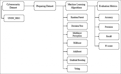
The proposed methodology described in this section was employed in this study to recognize distinct types of assaults in the UNSW-NB15 cybersecurity dataset, as depicted in Figure 1. The proposed methodology is demonstrated in the ensuing sections.
3.1 Dataset description
We used in our experiment a well-known dataset that has many cybersecurity attacks: the UNSW-NB15 dataset. Table 1 shows the name of each dataset, the number of Instances, the number of features, and what are the cybersecurity attacks.
The IXIA traffic generator uses three servers to generate this dataset: two servers for normal attacks and one server for malicious attacks. This dataset contains 45 features and 257,673 instances divided into 93,000 regular attacks and 164,673 malicious attacks [16]. The vicious attacks included nine attacks: Analysis, Reconnaissance, DoS, Exploits, Fuzzers, Generic, Normal, Worms, Backdoor, and Shellcode. The features of this dataset are shown in Table 2.
Figure 1. Diagram of the proposed methodology
Table 1. Information on cybersecurity datasets
|
Dataset Name |
No. of Instances |
No. of Features |
Cybersecurity Attacks |
|
UNSW-NB15 |
257,673 |
45 |
Analysis, Reconnaissance, DoS, Exploits, Fuzzers, Generic, Normal, Worms, Backdoor, Shellcode |
Table 2. UNSW-NB15 features
|
No. |
Feature |
No. |
Feature |
No. |
Feature |
|
1) |
id |
16( |
dloss |
31( |
response_body_len |
|
2) |
dur |
17( |
sinpkt |
32( |
ct_srv_src |
|
3) |
proto |
18( |
dinpkt |
33( |
ct_state_ttl |
|
4) |
service |
19( |
sjit |
34( |
ct_dst_ltm |
|
5) |
state |
20( |
djit |
35( |
ct_src_dport_ltm |
|
6) |
spkts |
21( |
swin |
36( |
ct_dst_sport_ltm |
|
7) |
dpkts |
22( |
stcpb |
37( |
ct_dst_src_ltm |
|
8) |
sbytes |
23( |
dtcpb |
38( |
is_ftp_login |
|
9) |
dbytes |
24( |
dwin |
39( |
ct_ftp_cmd |
|
10) |
rate |
25( |
tcprtt |
40( |
ct_flw_http_mthd |
|
11) |
sttl |
26( |
synack |
41( |
ct_src_ltm |
|
12) |
dttl |
27( |
ackdat |
42( |
ct_srv_dst |
|
13) |
sload |
28( |
smean |
43( |
is_sm_ips_ports |
|
14) |
dload |
29( |
dmean |
44( |
attack_cat |
|
15) |
sloss |
30( |
trans_depth |
45( |
label |
Table 3. Attack classes in UNSW-NB15 dataset
|
Attack |
Label |
Frequency |
|
Normal |
Normal |
93,000 |
|
Analysis |
Malicious |
2,677 |
|
Backdoor |
Malicious |
2,329 |
|
DoS |
Malicious |
16,353 |
|
Exploits |
Malicious |
44,525 |
|
Probing |
Malicious |
23,389 |
|
Fuzzers |
Malicious |
24,246 |
|
Generic |
Malicious |
58,871 |
|
Reconnaissance |
Malicious |
13,987 |
|
Shellcode |
Malicious |
1,511 |
|
Worms |
Malicious |
174 |
Furthermore, the classes and significant categories of cyber threats associated with those data, with their frequency and number of iterations, can be described in Table 3.
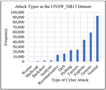
It is concluded from the data illustrated in Table 3 that the most frequent number of cyber threats associated with the UNSW-NB15 dataset is the Normal attack, corresponding to 93,000 cyber threats. In addition, the numeric data represented in Table 3 can be expressed as a graphical architecture via Figure 2.
Figure 2. UNSW-NB15 frequency attacks
It can be inferred from the data represented in Figure 2 that the Generic, Exploits, Fuzzers, Probing, and DoS Cyber Attacks come after the Normal attack in terms of frequency, contributing to iterations of 58,871, 44,525, 24,246, 23,389, and 16,353 attacks, respectively. At the same time, Worms and Shellcode have the least frequency of cyber threats, with a number of 174 and 1,511, respectively.
3.2 Dataset preparation
We use a well-known encoding approach to turn each dataset’s non-numerical features into numerical features to apply various machine-learning algorithms to them [17]. This method is known as the “Label Encoder,” and it turns non-numerical data into machine-readable forms by replacing each value with a unique number starting at 0 [17]. In the dataset, named UNSW-NB15, the proto, service, and state are categorical features. Therefore, we must convert it to numerical features. After that, the dataset was split into two datasets: a training dataset to build the models and a testing dataset to assess the performance of these models. The size of each dataset is as follows: 0.10 of the whole datasets is for testing and the remainder is a training dataset.
3.3 Main ML algorithms
To detect the aforementioned cybersecurity assaults in each dataset, the dataset is created and then fitted to seven machine learning algorithms. With a test size of 0.1, we used a hold-out approach to split the dataset into training and testing datasets. As a result, testing datasets account for 0.1 of all datasets, whereas training datasets make for 0.9 of them. The performance of the machine learning models created using the training dataset is assessed using the testing dataset.
3.3.1 Random Forest algorithm (RF)
A vast number of Decision Trees are trained in the ensemble supervised learning technique known as random forests, which is used for regression and classification applications. The class that most trees select is the predicted outcome in categorization problems. For regression tasks, the mean or average forecast of each tree is returned [18]. Decision Trees have the propensity to overfit their training set, which can be prevented using random-choice forests. To categorize any cybersecurity dataset, which includes a variety of assaults, the Random Forest classifier is used [19, 20]. Because the label in our experiment is discrete, we employed a Random Forest with a categorization type. Sqrt is the maximum number of features, none is the maximum depth, and 42 is the unexpected state. These are the RF settings that were used.
3.3.2 Decision Tree algorithm (DT)
A supervised machine learning system called a Decision Tree makes decisions based on rules, much like people do [21]. Data mining, statistics, and machine learning all use Decision Tree learning, also known as induction of Decision Trees, as a predictive modeling technique [22]. It moves from making observations about a sample (represented by the branches) to concluding the sample’s target value (represented by the attack-type leaves on a Decision Tree) [23]. Classification trees are tree models with a discrete target variable; in these tree structures, the leaves correspond to the many sorts of assaults, while the branches correspond to the characteristics of the dataset that help predict the class labels [24, 25]. Decision Trees with a continuous objective variable (usually real numbers) are known as regression trees [25]. Due to their clarity and simplicity, Decision Trees are one of the well-known machine learning algorithms. Because the label in our experiment is discrete, we utilized the Decision Tree with classification type. The DT settings we used were criterion=gini and random state=42.
3.3.3 Multilayer Perceptron algorithm (MLP)
A fully linked feedforward artificial neural network called a Multilayer Perceptron (MLP) is one type (ANN). The term “MLP” can apply to any feedforward ANN or networks made up of many layers of perceptrons, depending on the context (with threshold activation). The basic neural networks are multilayer perceptrons, especially those with a single hidden layer [26]. The minimum number of node levels for an MLP is an input layer, a hidden layer, and an output layer. Each node is a neuron with a nonlinear activation function, except the input nodes [26, 27]. MLP employs backpropagation as a supervised learning technique during training. MLP differs from a linear perceptron in that it uses nonlinear activation and has a large number of layers. It can distinguish between data that cannot be separated linearly [28]. Since the label in our experiment is discrete, we utilized the MLP with classification type, activation=relu, and random state=42.
3.3.4 eXtreme Gradient Boosting algorithm (XGBoost)
XGBoost, or extreme Gradient Boosting, is a technique for classification and regression issues. It has undergone careful parallelization and optimization for the gradient-boosting approach [29]. The training time is significantly decreased by parallelizing the entire boosting procedure. We train hundreds of models on various subsets of the training dataset instead of creating the best model that can be built using the data, and then we vote on the model that performs the best [29]. (As in traditional approaches). XGBoost frequently performs better than conventional Gradient Boosting methods [30]. You have access to a ton of inner parameters in the Python code that you may change for increased precision and accuracy [31].
This algorithm’s primary function is to transform Decision Trees, which are weak learners, into strong learners, which results in the strong learner producing the final prediction label (average of each prediction by week classifier). Numerous key characteristics of the XGBoost have been optimized [29-31]. 1) Parallelization: The model is built to operate concurrently across several CPU cores. 2) Regularization: To avoid overfitting, XGBoost provides a range of regularization penalties. Regularizations with penalties result in effective training, which permits the model to generalize effectively. Non-linearity: XGBoost can identify nonlinear data patterns and learn from them. 4) Cross-validation is available and has already been incorporated. 5) Scalability: XGBoost can run distributed, allowing you to manage massive volumes of data with the aid of distributed servers and clusters like Hadoop and Spark. Numerous programming languages are supported, including Julia, Python, C++, and Java. We utilized this technique with a classification type and the XGBoost settings of col sample by level=1, learning rate=0.1, gamma=0, n estimators=100, and random state=42 because the label in our experiment is discrete.
3.3.5 AdaBoost algorithm
A particular kind of statistical classification meta-algorithm is called AdaBoost or Adaptive Boosting. Combining it with a variety of different learning tactics can boost performance. The final output of the boosted classifier is merged with the output of additional learning algorithms, or “weak learners” [32]. In circumstances where prior classifiers misclassified them, AdaBoost adapts to the weak learners by modifying them as they come in. It might, in some cases, be less prone to the overfitting problem than other learning techniques. As long as a learner’s performance is marginally better than random guessing, even if they perform poorly individually, the final model will still condense to a potent learner [33]. AdaBoost has been shown to be effective in combining weak base learners (like decision stumps) with strong base learners (like deep Decision Trees), producing a model that is more accurate [34].
Before a learning algorithm works at its peak on a dataset, it must be configured with a number of different parameters, and most of them are more appropriate for certain issue kinds than others. The best out-of-the-box classifier is usually referred to as AdaBoost, which uses Decision Trees as weak learners [32-34]. The Decision Tree learning process employs information obtained from each stage of the AdaBoost approach to determine the relative “hardness” of each training sample. As a result, later trees focus on data that are harder to categorize [34]. Because the label in our experiment is discrete, we utilized AdaBoost with classification type, and the GB parameters we used are as follows: n estimators are 50, the learning rate is 1, the random state is 42, and the algorithm is SAMME.R.
3.3.6 Gradient Boosting algorithm (GB)
A technique of machine learning called Gradient Boosting has applications in regression and classification, among other things. It provides a prediction model in the form of several models of Decision Tree-based weak predictions [35]. A method called Gradient Boosting turns several weak learners (Decision Trees) into one powerful learner. Individual Decision Trees are poor learners in this situation [36]. Each tree in succession is connected to the one before it and works to fix the flaw of the one before it. Boosting algorithms are frequently time-consuming to train yet very accurate because of this sequential link. Slower learning models do better in statistical learning [35, 36]. Each new student in the group of weak learners fits into the residuals of the stage preceding them as the model gets better. The final model combines the findings from each phase to produce a potent learner. Utilizing a loss function, residuals are found. For instance, mean square error (MSE) and logarithmic loss (log loss) can be utilized in classification and regression, respectively. It’s crucial to understand that the model remains unchanged when a new tree is added. The additional Decision Tree matches the current model’s residuals [35-37]. Due to the discrete nature of the label in our experiment, we employed the GB with categorization type. We applied the following GB parameters: n estimators=100, learning rate=0.1, friedman mse criterion, subsample=1.0, and random state=42.
3.3.7 Voting algorithm
Voting classifiers are ensemble machine learning models that, after learning from a range of different models, predict an output (class) based on the output’s best likelihood of being the target class [38]. The output class with the highest votes will be revealed by adding the outputs of each classifier that was input into the voting classifier [39]. As opposed to creating separate, specialized models and evaluating their performance, we suggest creating a single model that trains on many models and predicts output according to the overall number of votes for each output class. Two voting processes are supported by Voting Classifier [40, 41]. 1) Hard voting: Each classifier is most likely to correctly forecast the projected output class that receives the most votes or the class that each classifier is most likely to correctly predict. 2) Soft voting: The forecast is made using an average of the likelihoods assigned to each output class and the class itself. Because the label for our experiment is discrete, we employed the voting with classification method. There were the following voting choices: The voting process uses hard voting, and the estimators are DT, RF, and XGB.
3.4 Simulation setting
This research depended on numerical calculations and simulation processes by virtue of the Python software package. In this software, a numeric code was developed and created to conduct a comparative analysis for the seven algorithms, which are:
A- Decision Tree (DT);
B- Random Forest (RF);
C- Gradient Boosting (GB);
D- XGBoost (XGB);
E- Multilayer Perceptron (MLP), and;
F- Voting.
The simulation process was accomplished via the numerical Python code to generate some statistical findings and vital outcomes associated with the seven algorithms addressed in this work.
3.5 Parameter adjustment
Based on the seven algorithms chosen in this article, this study relied on some parameters and critical variables that could help assess and examine those seven algorithms in terms of their performance and reliability. Therefore, some evaluation metrics and assessment measures were adopted. Those evaluation techniques include the following concepts:
a- Accuracy;
b- Precision;
c- Recall;
d- F1-Score.
The experimental results for each machine learning technique utilizing a cybersecurity dataset are summarized in this section based on four evaluation metrics.
4.1 Evaluation metrics
To evaluate the machine learning algorithms that were utilized, a few assessment criteria include accuracy, precision, recall, and f1-score [42]. The following are the formulas for these metrics: TP, TN, FP, and FN, respectively, stand for True Positives, True Negatives, False Positives, and False Negatives.
4.1.1 Accuracy
The most obvious performance indicator is the ratio of properly predicted samples to total samples, which is just a ratio of correctly predicted samples to total samples.
Accuracy $=\frac{\mathrm{TP}+\mathrm{TN}}{\mathrm{TP}+\mathrm{TN}+\mathrm{FP}+\mathrm{FN}}$ (1)
4.1.2 Precision
The proportion of accurately predicted positive tweets to all of the anticipated positive samples is known as precision:
Precision $=\frac{T P}{T P+F P}$ (2)
4.1.3 Recall
Is the ratio of correctly predicted positive samples to all projected positive samples?
Recall $=\frac{T P}{T P+F N}$ (3)
4.1.4 F1-score
F1-score is the weighted average of Precision and Recall.
F1- score $=2 * \frac{\text { Precision } * \text { Recall }}{\text { Precision }+ \text { Recall }}$ (4)
In this dataset, we applied three experiments to detect several types of attacks: 1) Binary classification (normal and malicious attack types). 2) Multiclass classification (malicious attack types). 3) Enhancement experiment on the second experiment. These experiments are done to know if each algorithm is able to distinguish between the malicious attack types in UNSW-NB15 dataset.
4.2 Binary classification experiment
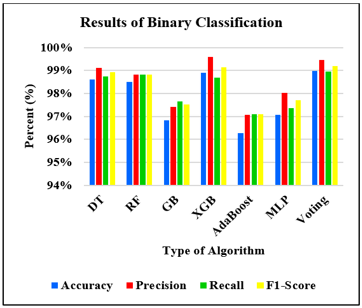
Machine learning methods are used in this experiment to determine if the sample in this dataset represents a legitimate attack or a malicious one. The performance results for the machine learning methods utilized are based on four metrics: precision, accuracy, f1-score, and recall, as shown in Table 4. In the detecting attack process, the Voting classifier outperforms the others with superior performance results.
It can be inferred from the data explained in Table 4 that the accuracy rates of the seven algorithms considered in this work range between a minimum value of 96.3% (which is for the AdaBoost algorithm) and a maximum value of 99.0% (which is related to the Voting algorithm). In addition, the precision ratios range from 97.1% to 99.6%, corresponding to AdaBoost and XGB algorithms, respectively. Further details and graphical illustrations pertaining to the results of assessment metrics and evaluation techniques of the seven algorithms are described in Figure 3.
It can be indicated from the data represented in Figure 3 (and Table 4) that the recall ratios linked to the seven algorithms are approximately closer together in terms of their proportions. The lowest recall ratio is recorded for the AdaBoost algorithm, corresponding to an amount of 97.1%. In contrast, the voting algorithm has the most significant portion, with a value of 98.9%. Also, the ultimate value of F1-Score was registered for the voting algorithm, recording a percentage of 99.2%.
Table 4. Performance results of binary classification
|
Algorithm Type |
Accuracy |
Precision |
Recall |
F1-Score |
|
DT |
98.6% |
99.1% |
98.7% |
98.9% |
|
RF |
98.5% |
98.8% |
98.8% |
98.8% |
|
GB |
96.8% |
97.4% |
97.6% |
97.5% |
|
XGB |
98.9% |
99.6% |
98.7% |
99.1% |
|
AdaBoost |
96.3% |
97.1% |
97.1% |
97.1% |
|
MLP |
97.1% |
98.0% |
97.4% |
97.7% |
|
Voting |
99.0% |
99.4% |
98.9% |
99.2% |
Figure 3. Performance results of binary classification
4.3 Multiclass classification experiment
The following forms of malicious software are used in this experiment: Analysis, Backdoor, DoS, Exploits, Fuzzers, Generic, Reconnaissance, Shellcode, and Worms. Precision, accuracy, f1-score, and recall are the four metrics on which the performance outcomes for the machine learning approaches used are based, as shown in Table 5 and Figure 4. The XGB algorithm surpassed the competition in terms of these metrics during the detection process.
It can be indicated from the data expressed in Table 5 that the accuracy rates of the seven algorithms considered in this work range between a minimum value of 57.5% (which is for the AdaBoost algorithm as in the first case) and a maximum value of 83.2% (which is related to the XGB algorithm). Besides, the precision percentages range from 50.2% to 80.5%, corresponding to AdaBoost and XGB algorithms, respectively (as in the first case). More details and graphical representations associated with the numerical outputs of evaluation techniques and assessment metrics of the seven intelligent algorithms can be described in Figure 4.
It can be inferred from the data expressed in Figure 4 (and Table 5) that the recall ratios regarding the seven algorithms are relatively approximate to each other according to their percentages. The maximum recall ratio is recorded for the XGB algorithm, corresponding to an amount of 65.3%. On the other hand, the AdaBoost algorithm has the weakest portion, with a ratio of 40.1%. Besides, the F1-Score recorded a minimum percentage of 34.5% for the AdaBoost algorithm. In contrast, the XGB attained the maximum rate of F1-Score, providing an ultimate percentage of 68.8%.
Table 5. Performance results of multiclass classification
|
Algorithm Type |
Accuracy |
Precision |
Recall |
F1-Score |
|
DT |
80.2% |
62.4% |
62.7% |
62.5% |
|
RF |
82.1% |
66.2% |
61.2% |
63.0% |
|
GB |
82.0% |
77.4% |
61.7% |
65.6% |
|
XGB |
83.2% |
80.5% |
65.3% |
68.8% |
|
AdaBoost |
57.5% |
50.2% |
40.1% |
34.5% |
|
MLP |
80.1% |
73.9% |
48.5% |
53.0% |
|
Voting |
82.4% |
66.5% |
64.9% |
65.6% |
Figure 4. Performance results of multiclass classification
4.4 Enhancement experiment
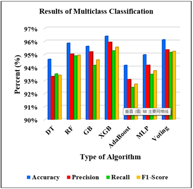
To improve the results of the second experiment, we apply the machine learning algorithms to three attacks (Generic, Fuzzers, and Exploits) because the models faced difficulty in detecting one of the nine attacks, and the number of samples in deleted attacks is small. Table 6 displays the performance results of these algorithms for three network attacks. Even yet, the XGB algorithm outperformed the competition in terms of these parameters during the detection procedure.
It is concluded from the obtained in Table 6 that the accuracy rate of the seven algorithms investigated and implemented in this research ranges from a minimum amount of 94.2% (which is for the AdaBoost algorithm as in the previous cases) and a maximum percentage of 96.4% (which is related to the XGB algorithm similar to the previous scenarios). Besides, the precision percentages range between 93.1% to 95.9%, corresponding to AdaBoost and XGB algorithms, respectively (as in previous cases). Also, a graphical representation of those numerical evaluation data can be expressed in Figure 5.
It can be inferred from the numeric information expressed in Figure 5 (and Table 6) that the recall ratios regarding the seven algorithms are relatively approximate to each other according to their percentages. However, the AdaBoost algorithm offered the least balance of recall, with a percentage of 92.5%. Meantime, the XGB algorithm recorded the maximum portion of recall compared with all five algorithms, with a rate of 95.3%. Furthermore, the AdaBoost has also registered the minimum F1-Score rate of 92.7% compared with the 95.6%, which is associated with the XGB algorithm (as well). This value is the ultimate amount of all ratios obtained in the F1-Score evaluation results.
Table 6. Performance results of multiclass classification with three attacks
|
Algorithm Type |
Accuracy |
Precision |
Recall |
F1-Score |
|
DT |
94.6% |
93.3% |
93.5% |
93.4% |
|
RF |
95.9% |
95.0% |
94.9% |
94.9% |
|
GB |
95.6% |
95.2% |
94.2% |
94.6% |
|
XGB |
96.4% |
95.9% |
95.3% |
95.6% |
|
AdaBoost |
94.2% |
93.1% |
92.5% |
92.7% |
|
MLP |
95.0% |
94.2% |
93.5% |
93.7% |
|
Voting |
96.1% |
95.3% |
95.1% |
95.2% |
Figure 5. Performance results of multiclass classification with three attacks
This research is guided to examine the critical role and major contributions of ML and DL principles in achieving considerable accuracy and effectiveness in cyber threat detection. Seven ML algorithms were selected, which were: DT, RF, GB, XGB, AdaBoost, MLP, and voting to detect network attacks in the information security field. The first step, the UNSW-NB15 dataset, is studied in this paper related to various types of network attacks. Second, the dataset was prepared for use in machine learning methods so that many models could be created. For example, each dataset’s non-numerical features were converted to numerical features using the “Label Encoder” encoding method, which is a well-known encoding approach. In this dataset, we applied three experiments to detect several types of attacks: 1) Binary classification (normal and malicious attack types). 2) Multiclass classification (malicious attack types). 3) Enhancement experiment on the second experiment. These experiments are done to know if each algorithm is able to distinguish between the malicious attack types in UNSW-NB15 dataset. The results shown in three experiments are as follows: 1. The Voting classifier outperforms the higher performance results compared with the others in the detection attack process. 2. The XGB algorithm achieved better performance results in the evaluation metrics in the detection process compared with the others. 3. Even yet, the XGB algorithm outperformed the competition in terms of performance measures used in the detection process.
It is worth mentioning that the practical implications of this work and the managerial benefits and real-life importance of those numerical simulations and evaluation analyses are reflected in the following aspects:
A- Providing better practices and robust approaches to cyber threats detection and internet attacks identification with enhanced levels of performance, reliability, accuracy, speed, and trustworthiness;
B- Supporting businesses, managers, and investment owners in protecting their private data and achieving better rates of information security;
C- Offering reliable and flexible techniques of cyber threat determination to save financial resources and customers’ private data without affecting companies’ security and safety in terms of data storage and information dependability;
D- Preventing any damage or harmful threats that could affect firms and organizations and might disrupt their secretive databases or employees’ information;
E- Providing beneficial tools and more effective tactics and strategies for detecting cyber threats quickly with the help of innovative ML and DL principles compared with traditional methods and slower approaches to internet attack identification.
[1] Xiong, F., Zang, L.Z., Gao, Y.Y. (2022). Internet penetration as national innovation capacity: Worldwide evidence on the impact of ICTs on innovation development. Information Technology for Development, 28(1): 39-55. https://doi.org/10.1080/02681102.2021.1891853
[2] Ahmetoglu, S., Che Cob, Z., Ali, N.A. (2022). A systematic review of internet of things adoption in organizations: Taxonomy, benefits, challenges and critical factors. Applied Sciences, 12(9): 4117. https://doi.org/10.3390/app12094117
[3] Schuh, G., Jarke, M., Gützlaff, A., Koren, I., Janke, T., Neumann, H. (2022). Review of commercial and open technologies available for industrial Internet of Things. In Design and Operation of Production Networks for Mass Personalization in the Era of Cloud Technology, 209-241. https://doi.org/10.1016/B978-0-12-823657-4.00005-1
[4] Veit, R.D. (2022). Safeguarding regional data protection rights on the global Internet-the European approach under the GDPR. In Personality and Data Protection Rights on the Internet: Brazilian and German Approaches, Cham: Springer International Publishing, 445-484. https://doi.org/10.1007/978-3-030-90331-2_18
[5] Velani, A.F., Narwane, V.S., Gardas, B.B. (2023). Contribution of internet of things in water supply chain management: A bibliometric and content analysis. Journal of Modelling in Management, 18(2): 549-577. https://doi.org/10.1108/JM2-04-2021-0090
[6] Hillman, V. (2022). Data privacy literacy as a subversive instrument to datafication. International Journal of Communication, 16: 767-788.
[7] Walter, L., Denter, N.M., Kebel, J. (2022). A review on digitalization trends in patent information databases and interrogation tools. World Patent Information, 69: 102107. https://doi.org/10.1016/j.wpi.2022.102107
[8] Zwilling, M., Klien, G., Lesjak, D., Wiechetek, Ł., Cetin, F., Basim, H.N. (2022). Cyber security awareness, knowledge and behavior: A comparative study. Journal of Computer Information Systems, 62(1): 82-97. https://doi.org/10.1080/08874417.2020.1712269
[9] Baydoğmuş, G.K. (2021). The effects of normalization and standardization an Internet of Things attack detection. Avrupa Bilim Ve Teknoloji Dergisi, 29: 187-192. https://doi.org/10.31590/ejosat.1017427
[10] Anwer, M., Khan, S.M., Farooq, M.U. (2021). Attack detection in IoT using machine learning. Engineering, Technology & Applied Science Research, 11(3): 7273-7278. https://doi.org/10.48084/etasr.4202
[11] Ferriyan, A., Thamrin, A.H., Takeda, K., Murai, J. (2021). Generating network intrusion detection dataset based on real and encrypted synthetic attack traffic. Applied Sciences, 11(17): 7868. https://doi.org/10.3390/app11177868
[12] Pelletier, Z., Abualkibash, M. (2020). Evaluating the CIC IDS-2017 dataset using machine learning methods and creating multiple predictive models in the statistical computing language R. International Research Journal of Advanced Engineering and Science, 5(2): 187-191.
[13] Kumar, V., Sinha, D., Das, A.K., Pandey, S.C., Goswami, R.T. (2020). An integrated rule based intrusion detection system: analysis on UNSW-NB15 data set and the real time online dataset. Cluster Computing, 23: 1397-1418. https://doi.org/10.1007/s10586-019-03008-x
[14] Amaizu, G.C., Nwakanma, C.I., Lee, J.M., Kim, D.S. (2020). Investigating network intrusion detection datasets using machine learning. In 2020 International Conference on Information and Communication Technology Convergence (ICTC), IEEE, 1325-1328. https://doi.org/10.1109/ICTC49870.2020.9289329
[15] Kasongo, S.M., Sun, Y. (2020). Performance analysis of intrusion detection systems using a feature selection method on the UNSW-NB15 dataset. Journal of Big Data, 7: 1-20. https://doi.org/10.1186/s40537-020-00379-6
[16] Moustafa, N., Slay, J. (2015). UNSW-NB15: A comprehensive data set for network intrusion detection systems (UNSW-NB15 network data set). In 2015 Military Communications and Information Systems Conference (MilCIS), IEEE, 1-6. https://doi.org/10.1109/MilCIS.2015.7348942
[17] Hancock, J.T., Khoshgoftaar, T.M. (2020). Survey on categorical data for neural networks. Journal of Big Data, 7(1): 1-41. https://doi.org/10.1186/s40537-020-00305-w
[18] Pal, M. (2005). Random forest classifier for remote sensing classification. International Journal of Remote Sensing, 26(1): 217-222. https://doi.org/10.1080/01431160412331269698
[19] Farnaaz, N., Jabbar, M.A. (2016). Random forest modeling for network intrusion detection system. Procedia Computer Science, 89: 213-217. https://doi.org/10.1016/j.procs.2016.06.047
[20] Idhammad, M., Afdel, K., Belouch, M. (2018). Detection system of HTTP DDoS attacks in a cloud environment based on information theoretic entropy and Random Forest. Security and Communication Networks, 2018. https://doi.org/10.1155/2018/1263123
[21] Kingsford, C., Salzberg, S.L. (2008). What are decision trees? Nature Biotechnology, 26(9): 1011-1013. https://doi.org/10.1038/nbt0908-1011
[22] Quinlan, J.R. (1986). Induction of decision trees. Machine Learning, 1: 81-106. https://doi.org/10.1007/BF00116251
[23] De Ville, B. (2013). Decision trees. Wiley Interdisciplinary Reviews: Computational Statistics, 5(6): 448-455. https://doi.org/10.1002/wics.1278
[24] Amor, N.B., Benferhat, S., Elouedi, Z. (2004). Naive bayes vs decision trees in intrusion detection systems. In Proceedings of the 2004 ACM Symposium on Applied Computing, 420-424. https://doi.org/10.1145/967900.967989
[25] Kotsiantis, S.B. (2013). Decision trees: A recent overview. Artificial Intelligence Review, 39: 261-283. https://doi.org/10.1007/s10462-011-9272-4
[26] Noriega, L. (2005). Multilayer perceptron tutorial. School of Computing. Staffordshire University, 4(5): 444.
[27] Tang, J.X., Deng, C.W., Huang, G.B. (2015). Extreme learning machine for Multilayer Perceptron. IEEE Transactions on Neural Networks and Learning Systems, 27(4): 809-821. https://doi.org/10.1109/TNNLS.2015.2424995
[28] Ramchoun, H., Ghanou, Y., Ettaouil, M., Janati Idrissi, M.A. (2016). Multilayer perceptron: architecture optimization and training. International Journal of Interactive Multimedia and Artificial Intelligence, 4(1): 26-30. https://doi.org/10.9781/ijimai.2016.415
[29] Mitchell, R., Frank, E. (2017). Accelerating the XGBoost algorithm using GPU computing. PeerJ Computer Science, 3: e127. https://doi.org/10.7717/peerj-cs.127
[30] Pan, B.Y. (2018). Application of XGBoost algorithm in hourly PM2.5 concentration prediction. In IOP Conference Series: Earth and Environmental Science, IOP publishing, 113: 012127. https://doi.org/10.1088/1755-1315/113/1/012127
[31] Dong, W., Huang, Y.M., Lehane, B., Ma, G.W. (2020). XGBoost algorithm-based prediction of concrete electrical resistivity for structural health monitoring. Automation in Construction, 114: 103155. https://doi.org/10.1016/j.autcon.2020.103155
[32] Hu, W., Hu, W.M. (2005). Network-based intrusion detection using adaboost algorithm. In the 2005 IEEE/WIC/ACM International Conference on Web Intelligence (WI'05), IEEE, 712-717. https://doi.org/10.1109/WI.2005.107
[33] Jabri, S., Saidallah, M., El Alaoui, A.E.B., El Fergougui, A. (2018). Moving vehicle detection using haar-like, LBP and a machine learning adaboost algorithm. In 2018 IEEE International Conference on Image Processing, Applications and Systems (IPAS), 121-124. https://doi.org/10.1109/IPAS.2018.8708898
[34] Yuan, L., Zhang, F. (2009). Ear detection based on improved adaboost algorithm. In 2009 International Conference on Machine Learning and Cybernetics, IEEE, 4: 2414-2417. https://doi.org/10.1109/ICMLC.2009.5212166
[35] Son, J., Jung, I., Park, K., Han, B. (2015). Tracking-by-segmentation with online gradient boosting decision tree. In 2015 IEEE International Conference on Computer Vision (ICCV), 3056-3064. https://doi.org/10.1109/ICCV.2015.350
[36] Peter, S., Diego, F., Hamprecht, F.A., Nadler, B. (2017). Cost efficient gradient boosting. In 31st Conference on Neural Information Processing Systems, 1-11.
[37] Lusa, L. (2017). Gradient boosting for high-dimensional prediction of rare events. Computational Statistics & Data Analysis, 113: 19-37. https://doi.org/10.1016/j.csda.2016.07.016
[38] Kumar, U.K., Nikhil, M.B.S., Sumangali, K. (2017). Prediction of breast cancer using voting classifier technique. In 2017 IEEE International Conference on Smart Technologies and Management for Computing, Communication, Controls, Energy and Materials (ICSTM), 108-114. https://doi.org/10.1109/ICSTM.2017.8089135
[39] El-Kenawy, E.S.M., Ibrahim, A., Mirjalili, S., Eid, M.M., Hussein, S.E. (2020). Novel feature selection and voting classifier algorithms for COVID-19 classification in CT images. IEEE Access, 8: 179317-179335. https://doi.org/10.1109/ACCESS.2020.3028012
[40] Khan, M.A., Khan Khattk, M.A., Latif, S., Shah, A.A., Ur Rehman, M., Boulila, W., Driss, M., Ahmad, J. (2022). Voting classifier-based intrusion detection for IoT networks. In Advances on Smart and Soft Computing: Proceedings of ICACIn, Springer Singapore, 2021: 313-328. https://doi.org/10.1007/978-981-16-5559-3_26
[41] Mahabub, A. (2020). A robust technique of fake news detection using ensemble voting classifier and comparison with other classifiers. SN Applied Sciences, 2(4): 525. https://doi.org/10.1007/s42452-020-2326-y
[42] Dalianis, H. (2018). Evaluation metrics and evaluation. Clinical Text Mining: Secondary Use of Electronic Patient Records, 45-53. https://doi.org/10.1007/978-3-319-78503-5_6