Hananta Diatmaja![]() | Aditya Rio Prabowo*
| Aditya Rio Prabowo*![]() | Ristiyanto Adiputra
| Ristiyanto Adiputra![]() | Nurul Muhayat
| Nurul Muhayat![]() | Seung Jun Baek
| Seung Jun Baek![]() | Nurul Huda
| Nurul Huda![]() | Tuswan Tuswan
| Tuswan Tuswan![]() | Achmad Zubaydi
| Achmad Zubaydi![]() | Haris Nubli
| Haris Nubli![]()
© 2023 IIETA. This article is published by IIETA and is licensed under the CC BY 4.0 license (http://creativecommons.org/licenses/by/4.0/).
OPEN ACCESS
As one of the world's largest archipelagic nations, Indonesia is tasked with the crucial responsibility of supervising and protecting its territorial waters from threats such as illegal fishing and damage to coral reefs. The effective and efficient execution of this task relies heavily on the use of fast patrol boats. Consequently, the need to investigate the hydrodynamic characteristics of these boats’ hulls is paramount. This study is primarily focused on the analysis and design of fast patrol boat hull prototypes. Our objective is to ascertain a practical design methodology that yields the optimal shape and size of the boat's hull. The adopted research methodology involved the design and analysis of eleven hull prototypes, evaluated based on resistance, stability, and seakeeping criteria. Five models were adapted from the reference ship, with a deadweight tonnage (DWT) variation of 2-3.5 tons. Three models employed the regression method with a block coefficient (CB) variation of 0.45-0.46, while the remaining three models utilized the scaling method, derived from the reference ship with the lowest resistance. The models in both the regression and scaling methods applied the primary size derived from the linear regression results of the five reference vessels. From the analysis, it was found that models developed using the regression method demonstrated superior hydrodynamic characteristics, denoted by consistently higher total values. This research provides valuable insights for the development of efficient fast patrol boats, which is crucial for the effective management of Indonesia's expansive maritime territory.
patrol boat, design method, resistance, stability, seakeeping
As the world's largest archipelagic nation, Indonesia is composed of 17,508 islands, including Sumatra, Java, Kalimantan, Sulawesi, Maluku, and Papua [1]. Historically, as an archipelagic country, Indonesia has been a significant producer of essential commodities for the global community, making its territory a focal point of international interest [2]. Threats to its maritime sector, such as illegal fishing and coral reef damage, pose serious risks to the aquatic ecosystem. In addition to overseeing its vast water areas, ports play a strategic role in facilitating the transport system that connects regions and countries [3]. Economically, ports serve as distribution channels for production, and socially, they function as interaction points for users [4]. Consequently, it is incumbent upon Indonesia to supervise and safeguard its water areas and ports, with a robust fleet serving as the primary means of addressing threats within the territory of the Unitary State of the Republic of Indonesia.
Indonesia is home to local shipyards that construct various fast patrol boats, and specific shipyards, such as PT. PAL Indonesia, are equipped to build corvettes, LPDs, and submarines [5]. Patrol boats form an essential part of the fleet, designed to supervise and guard the coast and waters. These boats are engineered to attain high speed and maintain good stability. Planing vessels, which are superficial in design and easier to assess performance-wise than multihulls, hydrofoil crafts, and hovercrafts, are commonly used for patrol, coast guard, and minor naval operations [6, 7]. The design of a planing patrol boat necessitates hydrodynamic analysis and prototype creation.
The hull prototype is scaled from the actual ship, making accuracy a paramount concern. Any error would be magnified when the prototype object is scaled to its actual size [8]. Hence, detailed planing for modeling is essential. The conversion of the primary size of the ship to a smaller size must consider multiple views, including the Plan View (from above), Elevation View (from the side), Section View (interior), Perspective View (perspective object), and Exploded View (order of assembly). To verify the analysis results without incurring high costs, a prototype ship is created based on the actual-size ship. A hydrodynamic analysis conducted on the ship prototype should be comparable to that of the actual-size ship, enabling the detection of design errors. Previous research on the hull prototype focused on the impact of hull modification on resistance values [9]. Investigations of the hull, based on resistance criteria, utilized the Holtrop regression method and the Savitsky mathematical model [10]. The design characteristics of a monohull, serving as a medical and logistical vessel for COVID-19, were also analyzed [11].
The application of hull prototypes can serve as a valuable aid in facilitating human tasks. Prior research has centered on the finite element analysis (FEA) of autonomous Unmanned Surface Vehicles (USV) for fish-feeding vessels [12]. Ship prototypes are also employed for scientific competitions, fostering research development related to hull design. Investigations involving ship prototypes aim to develop an efficient hull design model anchored on hydrodynamic characteristics, thereby envisaging the prototype's transformation into a real boat through meticulous planing.
The preliminary phase in the fundamental design of a ship entails the formulation of a design concept and initial configuration. The design concept is ascertained by understanding the primary dimensions of the boat. These dimensions, which include overall length, beam, draft, power, and speed, can be estimated using a regression method, with each dimension regressed to deadweight [13]. After determining the primary size of the ship from the regression results, it is then scaled to the prototype size. Existing research has explored the comparison of hydrodynamic characteristics in regression and scaling methods without explicitly comparing these two methods. Hence, this study undertakes multiple variations of the primary ship size, such as the regression method and the scaling method, and conducts a comparative analysis with the reference ship.
This research concentrates on the alterations in hydrodynamic characteristics (resistance, stability, and seakeeping) in patrol boat design methods derived from reference ships, regression, and scaling methods. These are compared based on Multi-Attribute Decision Making. This study incorporates the analysis of the KN value in stability analysis, which typically utilizes Large Angle Stability in contemporary research. The objective of this research is to evaluate various design variations in accordance with the selected design method. Design variations are scrutinized based on hydrodynamic characteristics, with the aim to yield the optimal design. This could potentially serve as a reference in planing the realization of an actual ship, tailored to the needs of fast patrol boats. Hydrodynamic analysis employing Maxsurf software simulation encompasses resistance with the Savitsky planing method, stability in the form of KN value and large angle stability analysis, and seakeeping.
The design of the ship prototype is based on a reference ship that has been created by experts. This is because the ship design takes a long time to find a feasible design [14, 15]. So, it is enough to have a general concept based on the selected reference ship. In the early stages, hull and compartment modeling with parameters of overall length, beam, depth, and all the locations of the bulkheads that make up the compartment [16]. Determining the main size of the ship is the basis for designing a ship. The main size of the ship will also affect the shape and results of the hydrodynamic analysis. Mathematical models with regression analysis can determine the main size of the new ship based on several reference vessels [17]. The scaling method is used to convert the main dimensions of the actual ship to the size of the prototype.
2.1 Regression method
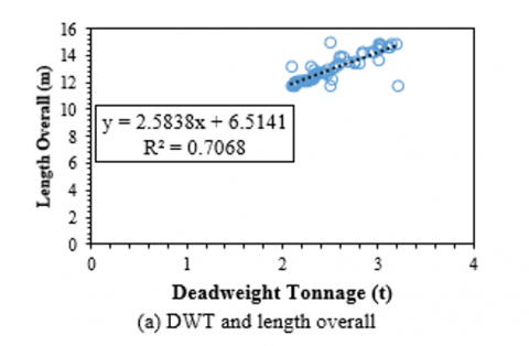
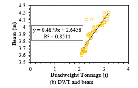
Regression analysis aims to analyze the correlation between several independent variables or predictors [18, 19]. There is a variable as a cause, for example, variable X and a variable as a result, for example variable Y. The ship design process can use regression analysis with one of the parameters as a fixed variable. So, length overall (LOA), beam (B), depth (D) has been regressed against deadweight tonnage (DWT). So that there is a straight line which is a relationship between several coordinates or variables is called linear regression. The straight line in this linear regression is like a gradient line that follows Eq. (1) [20].
$F(x)=a x+b$ (1)
where, F(x) as y. x and y are variables and a and b are constants.
2.2 Prototype scale
Ship size is the basic concept of ship scale [21]. The scale method can be used to make prototype on ship without changing the shape of the ship. So that the comparison between the actual size of the ship is comparable to the size of the ship prototype. The comparison includes length overall with beam (L/B), length overall with depth (L/D), and beam with depth (B/D). Prototype scale can be used as analysis, simulation, and evaluation directly and can be adapted to various algorithms for modelling [22]. Research on model prototypes can also hone the final design with modeling assumptions and simplification [23]. In previous research the ship model was also scaled into two ship models that have different main size ratio [24]. In addition, a prototype scale can also be carried out to analyze propeller based on actual size of ship’s propeller [25].
2.3 Ship resistance
Ship resistance is a force that is opposite to the direction of the ship's motion [26]. Ship drag is influenced by several factors including keel condition, submerged hull form at the bow and stern, wetted surface area, and length of waterline (LWL) [27]. Ship resistance must be predicted because drag is very important in ship hydrodynamics [28, 29]. Therefore, in the ship design stage, it is necessary to plan for ship resistance. The patrol boat hull must produce low ship resistance in order to have a high ship speed. Total resistance consists of frictional resistance, viscous pressure resistance, and wave resistance. The total resistance has the equation shown in Eq. (2) [30].
$R_T=R_F+R_{V P}+R_W$ (2)
where, RT is the total resistance, RF is the frictional resistance, RVP is the viscous pressure resistance, and RW is the wave resistance.
Frictional resistance is a function of the Reynolds number (Rn) and the residual resistance is a function of the Froude number (Fr) [31]. Frictional resistance is influenced by Reynolds number, water density, velocity, and wetted surface area. The equation for the Reynolds number and the coefficient of frictional resistance are shown in Eqs. (3) to (5) [31].
$R_n=\frac{V_s \times L W L}{v}$ (3)
$C_F=\frac{0.075}{\left(\log R_n-2\right)^2}$ (4)
$C_F=\frac{R_F}{0.5 \times \rho \times V^2 \times A_{w s}}$ (5)
where, Rn is the Reynolds number; V is speed (m/s); v is the viscosity of water (m2/s); LWL is the length of the waterline (m); CF is the coefficient of frictional resistance; RF is frictional resistance (N); ρ is the density of water (kg/m3); Aws is wet hull surface (m2).
Viscous pressure resistance can affect the trim angle of the ship [32]. Viscous pressure resistance is included in the residual resistance on the ship. Equation of the coefficient of viscous drag and viscous resistance is shown in Eqs. (6) and (7) [33].
$1+k=\frac{C_V}{C_F}$ (6)
$C_V=\frac{R_F}{0.5 \times \rho \times V^2 \times A_{W S}} \times(1+k)$ (7)
where, 1+k is the ITTC57 correlation line depending on the Reynolds number [33].
Froude number is a dimensionless number that occurs in the flow around the ship's hull which functions to determine ship type criteria [34]. Froude number equation is shown in Eq. (8) [35].
$F_n=\frac{V}{\sqrt{g L}}$ (8)
where, v is the speed of the ship (m/s), g is the constant of gravity (9.8 m/s2), and L is the length of the ship (m).
Hydrodynamic characteristics of ships can be determined through numerical calculations including wetted surface, drag and resistance [36, 37]. Savitsky method was applied to the planing hull [38, 39]. Daniel Savitsky conducted research on ship hydrodynamics by estimating ship resistance and trim angle [40]. Daniel Savitsky's equation is shown in Eq. (9) [41].
$R_T=\Delta \tan \tau+\frac{0.5 \rho V^2 \lambda b^2 C_F}{\cos \tau}$ (9)
where, $\tau$ is the trim angle, and CF is the coefficient of frictional resistance.
2.4 Ship stability
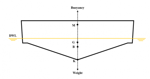
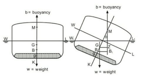
Stability Regulations of the International Maritime Organization (IMO) aim to improve ship safety based on safe ship stability [42]. Ship stability regulations have been determined for each of the different type of ship. In addition, IMO also discusses failures in stability including loss of stability, parametric roll, surf riding or broaching, dead ship conditions, and excessive acceleration [43]. This proves that the stability of the ship is one of the factors in the safety of the ship in sailing. There are important points in ship stability, namely the metacentric point (M), the buoyancy point (B), the gravity point (G), and the keel point (K). The location of the stability points is shown in Figure 1.
Figure 1. Stability points of ship
KN value or also called the cross curved of stability is the relationship between the righting arm and the displacement of a certain heel angle [44]. The value of KN depends on the geometry of the submerged volume and does not depend on the center of gravity. During each ship's journey, the condition of the cargo and the amount of ballast always change. So, the center of gravity (G) of the ship is not always fixed. KN value equation is shown in Eqs. (10) and (11) [44].
$K N=K N(\alpha, \Delta)$ (10)
$K N=G Z+K G \sin \sin \alpha$ (11)
GZ value is the perpendicular distance between the lines of action [45]. The higher the GZ value, the ship can be said to have good stability. This is because the ship has the maximum moment force to return to the upright position of the ship. International Maritime Organization issues ship stability regulations based on GZ values. This regulation is stated in Code A.749 (18) Chapter 3, Design Criteria Applicacle to All Ships [46].
2.5 Ship seakeeping
Ship seakeeping has an impact on the eligibility of ship passengers, the use of ships, the safety of ships, both merchant ships and naval vessels [47]. Seakeeping is the motion of the ship caused by the aquatic environment such as ocean waves. Ship movement behavior is very important to predict accurately at the ship design stage [48]. The complex marine environment is the main thing that needs to be considered in ship design. Seakeeping is a popular topic in ship architecture but has not been able to obtain maximum results due to the complexity of the fluid structure, amplitude of motion, and ship speed [49]. The ship experiences movement due to wave treatment, namely displacement movements (swaying, heaving, surging) and angular movements (pitching, rolling, yawing).
2.6 Multi-attribute decision making
Multi Attribute Decision Making is a method of making conclusions or in the form of decisions based on attributes or criteria used as boundaries [50]. This method uses a simple weighting called Simple Additive Weighting (SAW) which is usually used by practitioners [51]. The SAW method has a basic concept by adding up the weights based on performance ratings. This method requires data normalization so that it can be compared to all existing alternatives. The normalization equation is shown in Eqs. (12) and (13).
$r_{i j}=\left\{\begin{array}{l}\frac{x_{i j}}{\operatorname{Max}_i x_{i j}} \\ \frac{\operatorname{Min}_i x_{i j}}{x_{i j}}\end{array}\right.$ (12)
$V_i=\sum_{i=1}^n w_i r_{i j}$ (13)
where, V is the preference value, w is the criterion weight, and r is the alternative normalized value.
The research method consists of several stages: data collection, data processing, simulation design, and data analysis. The reference vessel was selected based on the actual vessel size in the data collection stage. The selection of reference ships is five patrol boats. Furthermore, the five reference ships did 3D modeling using the Maxsurf Modeler software. The five reference ship designs are scaled as a prototype with an overall length of 1 m. Then the design of the reference ship prototype carried out data processing with the regression approach method. This stage produces one primary ship size data from the regression results.
The next stage is to model three variations of the new hull according to the design needs. The modeling is done by using Maxsurf Modeler software. The primary size of the ship is the regression data from the five reference ship prototype designs. So, the three variations of the hull produce the same primary dimension of the boat with different hull shapes.
Next, three ship models were selected from the five reference ships for scale-down. It also requires Maxsurf Modeler software in the modeling. These three ship models use the primary size data from the regression results so that eleven models were made, including five reference ship prototype designs, three new ship prototype designs with regression results, and three ship prototype designs from five reference ship designs with regression results.
All ship prototype designs were simulated using the Maxsurf Resistance, Maxsurf Stability, and Maxsurf Motion software. The simulation results were analyzed based on the hydrodynamic characteristics consisting of the ship's total resistance, the boat's stability, and the seakeeping of the vessel. This research can evaluate the hull design method based on hydrodynamic characteristics.
3.1 Reference ship
The selected reference ship uses a patrol boat type. The main size of the ship must be determined before 3D modeling of the hull is carried out [52-55]. According to the patrol boat, the selected reference vessel is the type of hull that uses a v-hull. They have a large Deadweight Tonnage (DWT) ranging from 2-3.5 tons to be a reference in carrying out regression to make the regression results more accurate. Then have a comparison between Length Overall with Beam (LOA/B), Length Overall with Depth (LOA/D), and Beam with Depth (B/D), which are not too far from one hull to another, to produce a linear regression graph. The selection of a reference vessel also considers the lines plan a company has shown so that 3D hull modeling can be carried out. Five reference ships were selected with the main ship size specifications shown in Table 1.
Table 1. Specification of the main size of the reference ships
|
Parameters |
Type of Hull |
||||
|
High Speed Rescue Craft |
SMIT Patrol Boat |
Light Weight Rescue Craft |
Fast Police Boat |
Aresa 1300 S RHIB |
|
|
DWT (t) |
3.20 |
2.30 |
3.00 |
2.50 |
2.10 |
|
LOA (m) |
11.70 |
13.20 |
13.70 |
14.95 |
13.20 |
|
Beam (m) |
4.20 |
4.10 |
4.20 |
4.10 |
3.60 |
|
Depth (m) |
1.60 |
1.60 |
1.60 |
1.94 |
1.82 |
|
Draft (m) |
0.70 |
0.70 |
0.70 |
0.85 |
0.80 |
|
LWL (m) |
11.29 |
11.49 |
12.84 |
13.70 |
11.92 |
|
CB (-) |
0.435 |
0.530 |
0.435 |
0.421 |
0.454 |
|
Disp. (t) |
10.91 |
17.27 |
13.01 |
18.93 |
14.56 |
In general, several parameters in the ship's main dimensions are used as the basis for ship architecture. These parameters are as follows:
The process of modeling the hull 3D using the Maxsurf Modeler software. The dimensions of the five reference hulls are scaled to the prototype's size, which has an Overall Length of 1 m. The shape of the hull is designed based on the lines plan that has been made. The 3D design of the ship's hull is shown in Figure 2.
Figure 2. 3D hull design on reference ships
3.2 Regression method
The primary size of the ship can be determined by the regression method of the selected reference ship. The size is a variable relationship, namely DWT, which produces variables due to Overall Length, Beam, and Draft [16]. The regression method is a straight line formed due to several causal variables. The graph of the regression results of the five reference ships is shown in Figure 3. Five reference ships were obtained due to limited data in the form of a lines plan which is the secret of the patrol ship company. So, generating numbers is needed to produce strong regression results. Generate a number using the rand between functions with an upper and lower limit, namely the selected reference ship. This function is performed by taking random data, as much as 70 data, according to the primary size of the reference ship.
Figure 3 shows a graph of the linear regression results of the five reference ships. The regression uses a DWT target of 2.6 tons. So that the equation of each effect variable is obtained, which consists of Overall Length, Beam, Depth, and Draft, this equation is used to determine a new dimension specification for the hull shown in Table 2.
Table 2. The new main dimensions on patrol boat
|
Parameters |
Value |
|
|
Real Ship |
Prototype Ship |
|
|
Length Overall (m) |
13.37022 |
1.00 |
|
Beam (m) |
4.03166 |
0.30 |
|
Depth (m) |
1.71562 |
0.13 |
|
Draft (m) |
0.75174 |
0.06 |
Figure 3. Regression result graphs
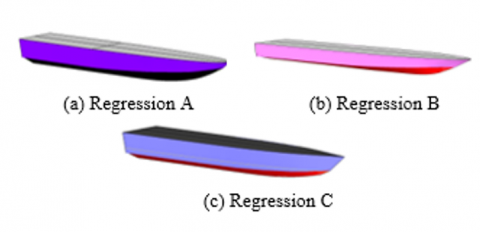
Figure 4. 3D hull design from regression results
The ship's main size specifications were used in the 3D modeling the new hull. The hull was made of three boats with the same primary size but different shapes. The primary dimension of the ship from the regression is done by scaling in the form of a prototype ship with an Overall Length of 1 m. The three hulls are Regression A, Regression B, and Regression C. The design of the three hulls is shown in Figure 4.
3.3 Scaling method
The design scale method was used for three hull prototypes selected from the reference ship based on the minor total ship resistance. The three hull prototypes used the regression results from the five reference ships shown in Table 2. The selected reference ship was simulated for resistance using Maxsurf Resistance software. The purpose of obstacle simulations is to choose the three best reference ships used for the scaling method in 3D modeling. Thus, three models will be taken from the five reference ships based on the smallest resistance value. It is necessary to properly compare with other design methods. The basic principle of the Savitsky method is a mathematical model that considers several possibilities that affect the ship's resistance. According to Savitsky, the aspect that most influence the value of drag is when the boat has a planing speed (Fr>1.5), which causes lift on the ship's bow, also called the trim angle or angle of attack in hydrodynamic theory. Therefore, at the trim angle, there is a frictional resistance related to the fluid viscosity force (Reynolds number).
The Savitsky total resistance formula is shown in Eq. (14).
$R_T=\Delta \tan \tau+\frac{1 / 2 \rho V^2 \lambda b^2 C_F}{\cos \tau \cos \beta}$ (14)
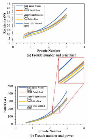
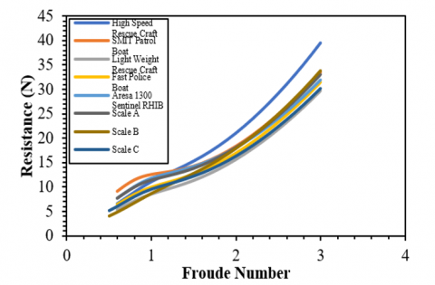
where, RT is total resistance, λ is the average value of the ratio between length and width in the wet area of the ship, ρ is water density, τ is the trim angle, b is the maximum chine beam, CF is friction coefficient, and β is deadrise angle. The results of the ship resistance simulation are the data shown in Table 3 and the graph in Figure 5.
Table 3. Resisatnce simulation results on reference ships
|
Fr. |
Resistance (N) |
||||
|
High Speed Rescue Craft |
SMIT Patrol Boat |
Light Weight Rescue Craft |
Fast Police Boat |
Aresa 1300 S RHIB |
|
|
0 |
0 |
0 |
0 |
0 |
0 |
|
0.5 |
0 |
0 |
0 |
0 |
0 |
|
1 |
10.99 |
12.61 |
8.61 |
9.89 |
11.75 |
|
1.5 |
15.23 |
14.31 |
11.39 |
12.56 |
14.15 |
|
2 |
20.97 |
18.36 |
15.67 |
16.86 |
18.02 |
|
2.5 |
29.10 |
24.87 |
21.83 |
23.20 |
24.02 |
|
3 |
39.49 |
33.46 |
29.72 |
31.38 |
31.92 |
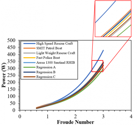
Based on the results of the resistance simulation, the three reference ship hulls have minor total resistance, namely Aresa 1300 Sentinel RHIB, Fast Police Boat, and Light Weight Rescue Craft. The total resistance of the ship at Froude number 1.5, respectively, is 14.15 N, 12.56 N, and 11.39 N. Meanwhile, the power required by the boat is 74.22 W, 66.36 W, and 60.91 W.
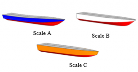
The three hulls are modeled using 3D modeling. The primary size of the ship regression results in the prototype's size. The hull designs were named Scale A (Aresa 1300 Sentinel RHIB), Scale B (Fast Police Boat), and Scale C (Light Weight Rescue Craft). The new design of the three reference vessels with regression outcome measures is shown in Figure 6.
Figure 5. Reference ship resistance simulation results graph
Figure 6. 3D hull design from scaling results
3.4 Ship simulation
The hull prototype design process resulted in eleven models. The full design consists of five reference hull prototypes, three hull prototypes resulting from the regression method with different hull shapes, and three scaling hull prototypes selected from the five reference vessels based on the minor total drag. The linear regression method produces one primary ship size based on the five reference ships. The main dimensions measure three new hull prototypes and three scaled hull prototypes. Then eleven models were simulated, including resistance, stability, and seakeeping, using Maxsurf software [56-59].
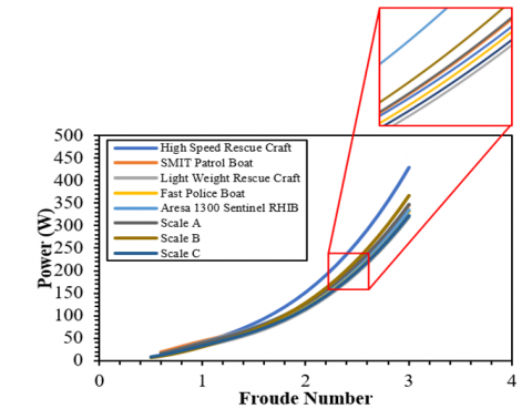
Ship resistance simulation using the Savitsky method at planing speed. The controlled variable used is the Froude number between zero and three with an interval of 0.5. This simulation produces a graph of the relationship between the Froude number and the required resistance and power. The goal is to determine the resistance and power needed against the Froude number. Therefore, the ship model with the minor total resistance with a small power can be selected.
Table 4. The similarities and differences between the KN value and Large Angle Stability analysis
|
Criteria |
KN Value |
Large Angle Stability |
|
Calculation location |
K to N |
G to Z |
|
Influenced |
Heel angle, Draft Amidship, Displacement increase |
Heel angle increase, Maximum Displacement |
|
Purpose |
Determine the KN value based on the increase in displacement at a certain heel angle |
Determine the GZ value at a certain displacement with respect to the increase in heel angle |
|
Utility |
To determine the level of stability based on displacement so that it can estimate the permissible displacement |
To find out the level of stability based on the heel angle so that one can estimate if the ship has a certain displacement, the heel angle must be considered |
|
Connection |
Directly proportional to the GZ value and in the direction of KG sin α (Heel Angle) |
Directly proportional to the KN value and opposite in the direction of KG sin α (Heel Angle) |
Ship stability simulation using KN Value (Cross Curve Stability) and Large Angle Stability analysis. Both analyses used a heel angle of 0° to 180° with an interval of 10°. In the KN Value analysis, input the displacement and draft amidships values according to the hydrostatic calculations in the Maxsurf Modeler software. This analysis produces a graph of the relationship between displacement and the importance of KN at a certain heel angle. At the same time, the study of Large Angle Stability has a graph of the relationship between the heel angle and the GZ value. The second purpose of this analysis is to determine the stability of the ship based on the standards of the International Maritime Organization (IMO). The similarities and differences between the KN value and Large Angle Stability analysis are shown in Table 4 and Figure 7.
Figure 7. Ship stability point
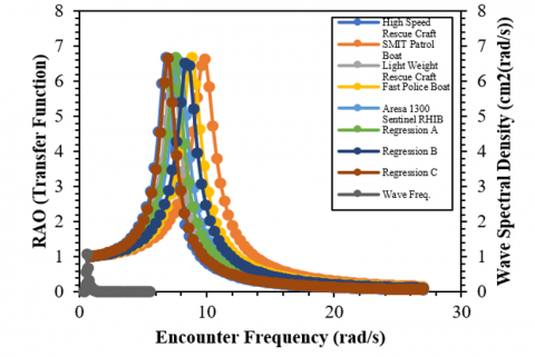
The following simulation analyzes ship seakeeping or ship motion using the strip theory method. The speed of the ship used is 10 knots, 20 knots, and 30 knots with variations in the angle of arrival of the waves, namely 90° (beam sea), 135° (bow quartering), and 180° (head sea). This simulation uses the wave spectrum of the Joint North Sea Wave Project (JONSWAP). Based on the simulation, the Response Amplitude Operator (RAO) graph includes heaving, rolling, and pitching. This analysis aims to determine the response of the ship's motion due to the influence of certain water wave conditions.
The statistical calculation process is carried out by comparing the three hull prototype design methods. The design method consists of a reference ship prototype, a new hull prototype design with the dimensions of the regression results, and the scaling method with the dimensions of the regression results. This calculation aims to analyze the use of the best design method based on the hydrodynamic characteristics of the ship, which include resistance, stability, and seakeeping.
The complete design of the hull prototype is compared between one method and another. Each simulation of the whole structure of the prototype hull of the ship is equalized. So, the simulation data can be compared based on the value of resistance, stability, and seakeeping. The analysis of the simulation results consists of a reference ship compared with the regression method, a reference ship compared with the scaling method, and a regression method compared with the scaling method.
The high ship speed influences the hull resistance value. The higher the rate of the ship, the greater the resistance generated. The method used in the simulation of resistance is the Savitsky method with planing speed. Generally, vessels that have high speed use this method. The parameter used is Froude number of zero to three with an interval of 0.5. In addition, the efficiency used is 85%. The analysis compares the three design methods based on the resistance value.
KN Value and Large Angle Stability analysis determine ship stability through stability simulation. KN Value analysis or cross curve stability is used to determine the ship's stability with different ship displacement parameters at each heel angle of the boat. While Large Angle Stability is used to determine the righting lever (GZ Value) based on the ship's total mass at each heel angle of the boat. The heel angle used is 0° to 180°. Ship displacement is obtained from hydrostatic calculations in Maxsurf Modeler software. Ship stability simulation using seawater density of 1,025 kg/m3.
4.1 Reference ship vs. regression method
The purpose of this comparison is to determine the effectiveness of the regression method that has been carried out. This study selected as many as five reference ship hulls to be compared by other design methods. Then from the five hulls, linear regression was carried out, which resulted in one primary size of the ship. Then, the main size of the regression results is scaled to the prototype size with an Overall Length of 1 m. The primary dimension of the ship is used in the regression design method by making three different hull prototype designs.
(a) Froude number vs. resistance
(b) Froude number vs. power
Figure 8. Graphics of simulation results of ship resistance on reference ships and regression method
Table 5. Simulation results of ship resistance on reference ships and regression method
|
Fr |
Resistance (N) |
|||||||
|
HSRC |
SMIT |
LWRC |
FPB |
ASR |
Reg. A |
Reg. B |
Reg. C |
|
|
0 |
0 |
0 |
0 |
0 |
0 |
0 |
0 |
0 |
|
0.5 |
0 |
0 |
0 |
0 |
0 |
0 |
0 |
0 |
|
1 |
10.99 |
12.61 |
8.61 |
9.89 |
11.75 |
9.54 |
9.81 |
10.13 |
|
1.5 |
15.23 |
14.31 |
11.39 |
12.56 |
14.15 |
11.82 |
12.84 |
12.54 |
|
2 |
20.97 |
18.36 |
15.67 |
16.86 |
18.02 |
15.51 |
17.36 |
16.48 |
|
2.5 |
29.10 |
24.87 |
21.83 |
23.20 |
24.02 |
21.09 |
23.98 |
22.43 |
|
3 |
39.49 |
33.46 |
29.72 |
31.38 |
31.92 |
28.36 |
32.51 |
30.18 |
Table 6. Simulation results of ship power on reference ships and regression method
|
Fr |
Power (W) |
|||||||
|
HSRC |
SMIT |
LWRC |
FPB |
Aresa |
Reg. A |
Reg. B |
Reg. C |
|
|
0 |
0 |
0 |
0 |
0 |
0 |
0 |
0 |
0 |
|
0.5 |
0 |
0 |
0 |
0 |
0 |
0 |
0 |
0 |
|
1 |
39.79 |
43.33 |
30.70 |
34.83 |
41.06 |
33.24 |
34.29 |
35.92 |
|
1.5 |
82.69 |
73.72 |
60.91 |
66.36 |
74.22 |
61.79 |
67.32 |
66.70 |
|
2 |
151.84 |
126.19 |
111.74 |
118.76 |
126.01 |
108.12 |
121.40 |
116.87 |
|
2.5 |
263.36 |
213.59 |
194.60 |
204.24 |
209.90 |
183.74 |
209.56 |
198.85 |
|
3 |
428.88 |
344.89 |
317.89 |
331.52 |
334.73 |
296.52 |
340.97 |
321.17 |
Table 7. Simulation results of ship stability on reference ships and regression method
|
Model |
Stability |
|||
|
Gz (cm) |
α (deg.) |
A (cm.deg.) |
Angle of Vanishing Point (deg.) |
|
|
High Speed Rescue Craft |
5.49 |
40.9 |
311.2 |
92.006 |
|
SMIT Patrol Boat |
5.66 |
36.4 |
324.7 |
89.935 |
|
Light Weight Rescue Craft |
4.19 |
41.8 |
235.0 |
90.841 |
|
Fast Police Boat |
3.61 |
42.7 |
211.2 |
90.971 |
|
Aresa 1300 Sentinel RHIB |
3.06 |
34.5 |
171.7 |
88.641 |
|
Regression A |
3.58 |
41.8 |
191.6 |
86.053 |
|
Regression B |
4.49 |
40.9 |
256.3 |
90.324 |
|
Regression C |
3.68 |
42.7 |
204.5 |
90.324 |
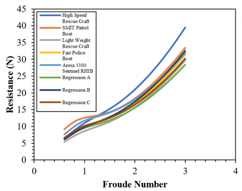
The simulation results of resistance and power in this comparison are shown in Tables 5 and 6. The simulation produces a graph of the relationship between Froude number and resistance and power which is shown in Figure 8.
Based on the simulation of the ship's resistance, different results were obtained from the two hull design methods. Sequentially, the hull prototypes that have total resistance from smallest to largest are Regression A, Light Rescue Boat, Regression C, Fast Police Boat, Aresa 1300 Sentinel RHIB, Regression B, SMIT Patrol Boat, and High-Speed Rescue Boat. The Regression A model has a total resistance of 28.36 N, and the required power is 296.52 W at Froude number 3. The Light Weight Rescue Craft model has a lower total resistance and power than Regression B and Regression C. The Light Weight Rescue Craft has a total resistance of 29.72 N, and the required power is 317.89 W at Froude number 3. Meanwhile, the model that has the highest total resistance and power is High-Speed Rescue Craft. The model is included in the reference ship, which has a total ship resistance of 39.49 N and a required power of 428.88 W. The data results show that the design method using linear regression does not always have a lower total resistance and power than the reference ship. But in this study, the method that produces the minor total resistance on the prototype hull is the regression design method. This can be caused by the influence of the shape of the hull on the primary size of the hull. In this comparison, the regression method tends to be more effective than the reference ship.
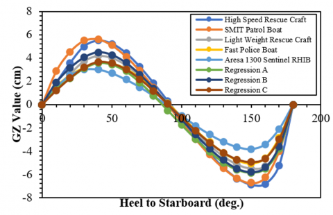
Furthermore, a comparison of the ship design method is carried out based on the ship's stability. Based on the simulation, a graph shows the GZ curve (righting lever). The graph shows the relationship between the GZ value and the ship's heel angle. The simulation results are shown in Table 7. and the righting lever graph is shown in Figure 9.
Figure 9. Graphics of simulation results of ship stability on reference ships and regression method
Based on the stability simulation, the results varied between the reference ship and the regression method. The ship hull prototype model that has the largest GZ value is the SMIT Patrol Boat model. This model has a GZ value of 5.66 cm with a maximum tilt angle of 36.4°. So, the SMIT Patrol Boat model has a maximum tilt limit of 36.4° to return to the ship's vertical position. The SMIT Patrol Boat Model is the ship model with the largest curve area on the righting lever chart. This model has a curve area of 324.7 cm.deg. Then the next model that has the largest curve area is the High-Speed Rescue Craft and Regression B models, each of which is 311.2 cm.deg and 256.3 cm. deg. Meanwhile, the model with the smallest curve area is the Aresa 1300 Sentinel RHIB. Based on these data, it can be concluded that the regression method does not always have good stability.
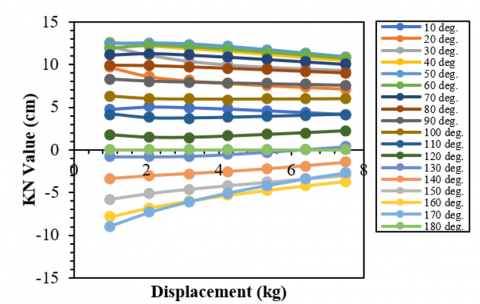
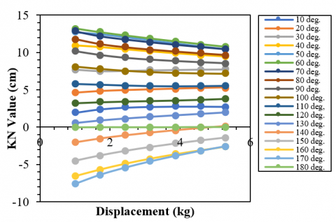
Simulation of KN value or cross curve stability is an analysis to measure ship stability at a certain displacement based on KN distance. The graph of the KN value simulation results shows the relationship between the KN value and displacement. The graph is shown in Figure 10.
(a) SMIT patrol boat
(b) High speed rescue craft
(c) Regression B
(d) Aresa 1300 sentinel RHIB
Figure 10. Graphics of cross curve stability
Figure 11. RAO heave motion graph between reference ships and regression method
Figure 12. RAO roll motion graph between reference ships and regression method
Figure 13. RAO pitch motion graph between reference ships and regression method
Seakeeping is a response to ship movements due to the influence of certain water waves. The hull design is vital because of the complexity of the water conditions. It affects the direction of the ship. So, the seakeeping analysis is needed to determine the response of the ship's motion to the waters. This analysis uses the angle of incidence of the waves, including 90°, 135°, and 180°, with variations in the speed of 10 knots, 20 knots, and 30 knots. Seakeeping simulation produces RAO graphs, including heave, roll, and pitch motions. The graph of RAO heave motion on the comparison of the reference ship to the regression method at the angle of incidence of the waves at 90° with a speed of 30 knots is shown in Figure 11.
Based on the RAO heave motion graph in Figure 11, it is found that the ship model that has the lowest motion response is Regression C. This model has a maximum RAO of 2.4 with a frequency of 16.65 rad/s. Meanwhile, the ship model that has the highest motion response is the SMIT Patrol Boat. This model has a maximum RAO of 4.39 with a frequency of 16.61 rad/s. All models have charts with the same trend in the heaving movement. Thus, the ship design method that has the lowest heave motion response is the regression method. Waves with an incident angle of 90° have a maximum value different from the wave frequency, so they don't experience superposition. Ships are more stable because they do not receive multiple waves simultaneously.
The graph of RAO roll motion on the comparison of the reference ship to the regression method at the angle of incidence of the waves at 90° with a speed of 30 knots is shown in Figure 12.
Roll movement is the movement of the ship to the right and left from the direction of the ship's speed. Based on the RAO roll motion graph, the model with the lowest RAO roll is obtained, namely Light Weight Rescue Craft. This model has a maximum RAO of 6.40 with a frequency of 7.47 rad/s. The Light Weight Rescue Craft has a lower rolling RAO than the Regression B model. The reference ship is superior to the regression method based on the simulated roll motion results. Waves do not experience superposition due to different peak frequencies, so the boat is more stable.
The graph of the RAO pitch motion on the comparison of the reference ship to the regression method at the angle of incidence of the waves at 90° with a speed of 30 knots is shown in Figure 13.
Based on the seakeeping simulation, the RAO pitch motion graph shows the same trend between the reference ships with the regression method. The model that has the lowest RAO pitch motion is Regression C. This model has an RAO pitch motion of 0.09 with a frequency of 16.66 rad/s. Meanwhile, the model with the following lowest RAO pitch motion is the Light Weight Rescue Craft. The maximum value between wave frequency and RAO pitch motion of all ships shows the difference in frequency. So, the waves do not experience superposition. The boat is more stable because it is not simultaneously hit by more than one wave.
4.2 Reference ships vs. scaling method
The purpose of this comparison is to determine the effectiveness of the scaling method on reference vessels. The five reference hulls are to be compared by the scaling design method. Three reference ships were selected based on the required resistance and power values. The boat with the lowest resistance and power is a scaling model. The scaling ship models include the Aresa 1300 Sentinel RHIB, Fast Police Boat, and Light Weight Rescue Craft. The ship scaling model uses the primary size of the linear regression results from the five reference ships. The reference ship and scaling ship have dimensions in prototype size with an overall length of 1 m.
The simulation results of resistance and power in the comparison between the reference ship and the scaling method are shown in Tables 8 and 9. The simulation produces a graph of the relationship between the Froude number and the resistance and power shown in Figure 14.
Table 8. Simulation results of ship resistance on reference ships and scaling method
|
Fr |
Resistance (N) |
|||||||
|
HSRC |
SMIT |
LWRC |
FPB |
Aresa |
Scale A |
Scale B |
Scale C |
|
|
0 |
0 |
0 |
0 |
0 |
0 |
0 |
0 |
0 |
|
0.5 |
0 |
0 |
0 |
0 |
0 |
0 |
4.01 |
5.14 |
|
1 |
10.99 |
12.61 |
8.61 |
9.89 |
11.75 |
9.54 |
8.65 |
9.53 |
|
1.5 |
15.23 |
14.31 |
11.39 |
12.56 |
14.15 |
11.82 |
12.77 |
12.19 |
|
2 |
20.97 |
18.36 |
15.67 |
16.86 |
18.02 |
15.51 |
17.89 |
16.29 |
|
2.5 |
29.10 |
24.87 |
21.83 |
23.20 |
24.02 |
21.09 |
24.92 |
22.33 |
|
3 |
39.49 |
33.46 |
29.72 |
31.38 |
31.92 |
28.36 |
33.85 |
30.13 |
Table 9. Simulation results of ship power on reference ships and scaling method
|
Fr |
Power (W) |
|||||||
|
HSRC |
SMIT |
LWRC |
FPB |
Aresa |
Scale A |
Scale B |
Scale C |
|
|
0 |
0 |
0 |
0 |
0 |
0 |
0 |
0 |
0 |
|
0.5 |
0 |
0 |
0 |
0 |
0 |
0 |
7.26 |
9.16 |
|
1 |
39.79 |
43.33 |
30.70 |
34.83 |
41.06 |
9.54 |
31.31 |
33.99 |
|
1.5 |
82.69 |
73.72 |
60.91 |
66.36 |
74.22 |
11.82 |
69.33 |
65.23 |
|
2 |
151.84 |
126.19 |
111.74 |
118.76 |
126.01 |
15.51 |
129.53 |
116.20 |
|
2.5 |
263.36 |
213.59 |
194.60 |
204.24 |
209.90 |
21.09 |
225.56 |
199.07 |
|
3 |
428.88 |
344.89 |
317.89 |
331.52 |
334.73 |
28.36 |
367.59 |
322.42 |
The resistance simulation results show variations between reference vessels using the scaling method. The model with total resistance from the smallest to the largest sequentially is Light Weight Rescue Craft, Scale C, Fast Police Boat, Aresa 1300 Sentinel RHIB, Scale A, SMIT Patrol Boat, Scale B, and High-Speed Rescue Craft. The Light Weight Rescue Craft model has a lower total resistance than the Scale C model. Scale C has a total resistance of 30.13 N, and the required power is 322.42 W at Froude number 3. The Light Weight Rescue Craft has a total resistance of 29.72 N, and the required power is 317.89 W at Froude number 3. Meanwhile, the model with the highest total resistance and power is High-Speed Rescue Craft. The data results show that the scaling design method does not always have a lower total resistance and power than the reference vessel. This research method produces a minor total resistance on the prototype ship's hull, namely the reference ship. In this comparison, the reference vessel tends to be superior to the scaling method.
(a) Froude number vs. resistance
(b) Froude number vs. power
Figure 14. Graphics of simulation results of ship resistance on reference ships and scaling method
Based on the ship stability simulation, a graph shows the GZ (righting lever) curve. The graph shows the relationship between the GZ value and the ship's heel angle. The simulation results data are shown in Table 10. and the righting lever graph shown in Figure 15.
Table 10. Simulation results of ship stability on reference ships and scaling method
|
Model |
Stability |
|||
|
Gz (cm) |
α (deg.) |
A (cm.deg.) |
Angle of Vanishing Point (deg.) |
|
|
High Speed Rescue Craft |
5.49 |
40.9 |
311.2 |
92.006 |
|
SMIT Patrol Boat |
5.66 |
36.4 |
324.7 |
89.935 |
|
Light Weight Rescue Craft |
4.19 |
41.8 |
235.0 |
90.841 |
|
Fast Police Boat |
3.61 |
42.7 |
211.2 |
90.971 |
|
Aresa 1300 Sentinel RHIB |
3.06 |
34.5 |
171.7 |
88.641 |
|
Scale A |
4.01 |
32.7 |
226.6 |
88.771 |
|
Scale B |
4.20 |
43.6 |
238.0 |
92.380 |
|
Scale C |
3.67 |
43.6 |
204.6 |
91.100 |
Figure 15. Graphics of simulation results of ship stability on reference ships and scaling method
The comparison between the reference ship and the scaling ship found that the SMIT Patrol Boat model has the highest GZ value of 5.66 cm. The SMIT Patrol Boat model has a maximum slope of 36.4° to return to the vertical position of the ship. The next model with the highest GZ value is the High-Speed Rescue Craft of 5.49 cm with an angle of 40.9°. Scale A and B are in the third and fourth positions based on the highest GZ value. However, Scale B and C have the highest maximum slope angle of 43.6°. The SMIT Patrol Boat Model is the ship model with the largest curve area on the righting lever chart. This model has a curve area of 324.7 cm.deg. Then, the next model that has the largest curve area is the High-Speed Rescue Craft and Regression B models, each of which is 311.2 cm.deg. and 256.3 cm.deg. Meanwhile, the model with the smallest curve area is Aresa 1300 Sentinel RHIB. Based on these data, it can be concluded that the scaling method does not always have good stability.
(a) Scale A
(b) Scale B
(c) Scale C
Figure 16. Graphics of cross curve stability
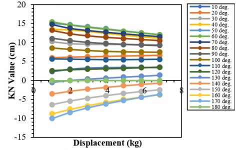
Cross-curve stability aims to measure the ship's stability at a particular displacement based on the KN distance. Displacement is taken from hydrostatic calculations on the hull prototype. The KN value simulation results graph shows the relationship between the KN value and displacement. The graph of the KN value in this comparison is shown in Figure 16.
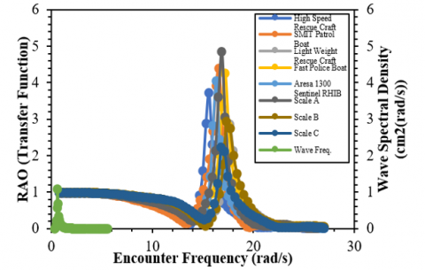
Water waves cause the ship to have a motion response consisting of heaving, rolling, and pitching. Seakeeping analysis is needed to determine the response of the ship's motion to complex water waves. This analysis uses the angle of incidence of the waves, including 90°, 135°, and 180°, with variations in the speed of 10 knots, 20 knots, and 30 knots. Seakeeping simulation produces RAO graphs, including heave, roll, and pitch motions. The graph of RAO heave motion on the comparison of the reference ship to the scaling method at an angle of 90° of wave incidence at a speed of 30 knots is shown in Figure 17.
Figure 17. RAO heave motion graph between reference ships and scaling method
Figure 18. RAO roll motion graph between reference ships and scaling method
Based on the RAO heave motion graph, it is found that the ship model has the lowest motion response, namely Scale C. This model has a maximum RAO heave motion of 2.24 with a frequency of 16.81 rad/s. At the same time, the ship model that has the highest motion response is Scale A. This model has a maximum RAO heave motion of 4.85 with a frequency of 16.88 rad/s. All models have charts with the same trend in the heaving movement. Thus, the ship design method with the lowest heave motion response is the scaling method, but in this comparison, the scaling method also has the highest heave motion response. Waves with an incident angle of 90° have a maximum value different from the wave frequency, so they don't experience superposition. Ships are more stable because they do not receive multiple waves simultaneously.
The graph of RAO roll motion on the comparison of the reference ship to the scaling method at an angle of 90° of wave incidence with a speed of 30 knots is shown in Figure 18.
Based on the RAO roll motion graph, the model with the lowest rolling RAO is Light Weight Rescue Craft. The model has a maximum RAO of 6.40 with a frequency of 7.47 rad/s. The Light Weight Rescue Craft has a lower rolling RAO than the Scale B model. Meanwhile, the model with the highest roll motion RAO is the High-Speed Rescue Craft of 6.67 with a frequency of 6.81 rad/s. The scaling model is not necessarily superior to the reference ship. The waves do not experience superposition due to the different peak frequencies, so the boat is more stable.
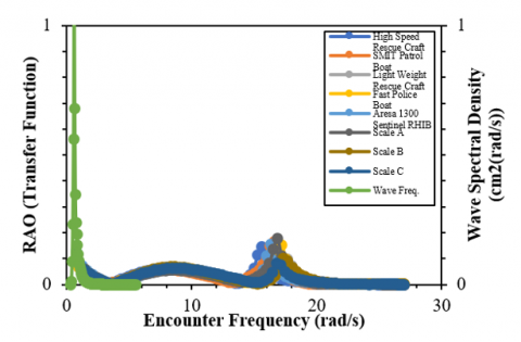
The graph of the RAO pitch motion on the comparison of the reference ship to the scaling method at an angle of 90° waves at a speed of 30 knots is shown in Figure 19.
Figure 19. RAO pitch motion graph between reference ships and scaling method
Based on the seakeeping simulation, the model has the lowest RAO pitch motion, Scale C. This model has an RAO pitch motion of 0.08 with a frequency of 16.81 rad/s. Meanwhile, the model with the following lowest RAO pitch motion is the Light Weight Rescue Craft. The Scale B model has nearly the same peak RAO pitch motion as the Light Weight Rescue Craft. The peak wave frequency with the RAO pitch motion of the entire ship shows the difference in frequency. So that the waves do not experience superposition which makes the boat more stable.
4.3 Regression method vs scaling method
These two methods were compared to determine the effectiveness of the regression and scaling methods. All models in these two methods have dimensional equations using the primary size of the ship from the regression results of the five selected reference ships. But the models in the regression and scaling methods have differences regarding the shape of the hull prototype. So, in this comparison, the best hull shape can be determined based on hydrostatic characteristics. The hull prototype of the regression method consists of Regression A, Regression B, and Regression C. The prototype of the hull of the scaling method consists of Scale A, Scale B, and Scale C. The three models in the scaling method are taken from the reference ship based on the resistance and power values required at most low. Scale A is born from the Aresa 1300 Sentinel RHIB model, Scale B from the High-Speed Rescue Craft model, and Scale C from the Light Weight Rescue Craft. The models in these two methods have dimensions in the prototype with an overall length of 1 m.
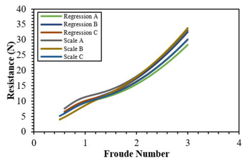
The simulation results of resistance and power in the comparison between the regression method and the scaling method are shown in Tables 11 and 12. The simulation produces a graph of the relationship between the Froude number and the resistance and power shown in Figure 20.
Table 11. Simulation results of ship resistance on regression method and scaling method
|
Fr |
Resistance (N) |
|||||
|
Reg. A |
Reg. B |
Reg. C |
Scale A |
Scale B |
Scale C |
|
|
0 |
0 |
0 |
0 |
0 |
0 |
0 |
|
0.5 |
0 |
0 |
0 |
0 |
4.01 |
5.14 |
|
1 |
9.54 |
9.81 |
10.13 |
9.54 |
8.65 |
9.53 |
|
1.5 |
11.82 |
12.84 |
12.54 |
11.82 |
12.77 |
12.19 |
|
2 |
15.51 |
17.36 |
16.48 |
15.51 |
17.89 |
16.29 |
|
2.5 |
21.09 |
23.98 |
22.43 |
21.09 |
24.92 |
22.33 |
|
3 |
28.36 |
32.51 |
30.18 |
28.36 |
33.85 |
30.13 |
Table 12. Simulation results of ship power on regression method and scaling method
|
Fr |
Power (W) |
|||||
|
Reg. A |
Reg. B |
Reg. C |
Scale A |
Scale B |
Scale C |
|
|
0 |
0 |
0 |
0 |
0 |
0 |
0 |
|
0.5 |
0 |
0 |
0 |
0 |
7.26 |
9.16 |
|
1 |
33.24 |
34.29 |
35.92 |
9.54 |
31.31 |
33.99 |
|
1.5 |
61.79 |
67.32 |
66.70 |
11.82 |
69.33 |
65.23 |
|
2 |
108.12 |
121.40 |
116.87 |
15.51 |
129.53 |
116.20 |
|
2.5 |
183.74 |
209.56 |
198.85 |
21.09 |
225.56 |
199.07 |
|
3 |
296.52 |
340.97 |
321.17 |
28.36 |
367.59 |
322.42 |
The model that has the total resistance from the smallest to the largest sequentially in this comparison is Regression A, Scale C, Regression C, Regression B, Scale A, and Scale B. Regression A has a lower total resistance than the Scale C model. 30 knots, Regression C has a curve that coincides with Scale C. But at the initial speed, Scale C has lower resistance than Regression C. The model that has the lowest resistance and power values is Regression A. The resistance of the Regression A model is 28.36 N with a power of 296.52 W. While the model with the highest resistance and power is Scale B with a magnitude of 33.85 N and 367.59 W, respectively. In this comparison, the regression method tends to be superior to the scaling method.
(a) Froude number vs. resistance
(b) Froude number vs. power
Figure 20. Graphics of simulation results of ship resistance on regression method and scaling method
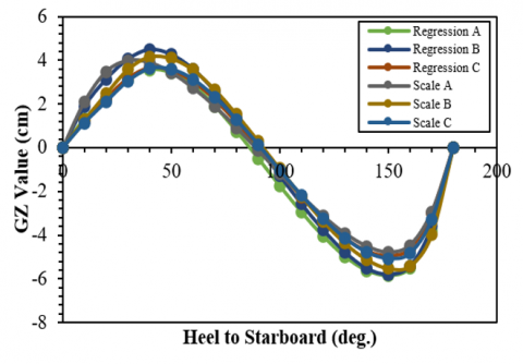
Based on the ship stability simulation, a graph shows the GZ (righting lever) curve. The graph shows the relationship between the GZ value and the ship's heel angle. The simulation results in data are shown in Table 13. The righting lever graph is in Figure 21.
In the comparison between the regression method and scaling, the Regression B model had the highest GZ value of 4.49 cm. This model has a maximum tilt limit of 40.9° to return to the vertical position of the ship. The next model with the highest GZ value is Scale B of 4.20 cm with an angle of 43.6°. But Scale B and C have the highest maximum tilt angle of 43.6°. Regression B is the ship model with the largest curve area on the righting lever chart. This model has a curve area of 256.3 cm.deg. Then the next model that has the largest curve area is Scale B and Scale A, each of which is 238 cm.deg. and 226.6 cm. deg. Meanwhile, the model that has the smallest curve area is Regression A. Based on these data, the scaling method is superior to the regression method based on the area under the curve and the maximum slope angle.
Table 13. Simulation results of ship stability regression method and scaling method
|
Model |
Stability |
|||
|
Gz (cm) |
α (deg.) |
A (cm.deg.) |
Angle of Vanishing Point (deg.) |
|
|
Regression A |
3.58 |
41.8 |
191.6 |
86.053 |
|
Regression B |
4.49 |
40.9 |
256.3 |
90.324 |
|
Regression C |
3.68 |
42.7 |
204.5 |
90.324 |
|
Scale A |
4.01 |
32.7 |
226.6 |
88.771 |
|
Scale B |
4.20 |
43.6 |
238.0 |
92.380 |
|
Scale C |
3.67 |
43.6 |
204.6 |
91.100 |
Figure 21. Graphics of simulation results of ship stability regression method and scaling method
Furthermore, ship stability is measured based on certain displacement conditions. This analysis is called Cross curve stability or KN value. The research aims to measure the ship's stability at a particular displacement based on the KN distance. Displacement is taken from hydrostatic calculations on the hull prototype. The KN value simulation results graph shows the relationship between the KN value and displacement. The graph of the KN value in this comparison is shown in Figure 22.
(a) Regression A
(b) Regression C
Figure 22. Graphics of cross curve stability
Seakeeping analysis is needed to determine the response of the ship's motion to complex water waves. This analysis uses the angle of incidence of the waves, including 90°, 135°, and 180°, with variations in the speed of 10 knots, 20 knots, and 30 knots. Seakeeping simulation produces RAO graphs, including heave, roll, and pitch motions. The graph of RAO heave motion on the comparison of the regression method with the scaling method at an incident angle of 90° waves with a speed of 30 knots is shown in Figure 23.
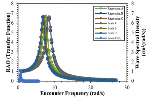
Figure 23. RAO heave motion graph between regression method and scaling method
Based on the RAO heave motion graph, values are obtained from lowest to highest sequentially: Scale C, Regression C, Scale B, Regression A, Regression B, and Scale A. The ship model that has the lowest motion response is Scale C. This model has a maximum RAO heave motion of 2.24 with a frequency of 16.81 rad/s. Regression C has a higher RAO heave motion than Scale C. Meanwhile, Scale A is the ship model with the highest motion response. This model has a maximum RAO heave motion of 4.85 with a frequency of 16.88 rad/s. The model in the scaling method has a higher average RAO heave motion than the regression method. Thus, the ship design method with the lowest heave motion response is the scaling method, but in this comparison, the scaling method also has the highest heave motion response. Waves with an incident angle of 90° have a maximum value different from the wave frequency, so they don't experience superposition. Ships are more stable because they do not receive multiple waves simultaneously.
The RAO roll motion graph on the comparison of the regression method with the scaling method at an angle of incidence of waves of 90° with a speed of 30 knots is shown in Figure 24.
Figure 24. RAO roll motion graph between regression method and scaling method
Based on the RAO roll motion graph, the model has the lowest to highest RAO rolling sequentially: Scale B, Regression B, Scale A, Scale C, Regression C, and Regression A. Model Scale B has a maximum RAO of 6.50 with a frequency of 6.97 rad/s. Regression B has a higher rolling RAO than the Scale B model. Meanwhile, the model with the highest RAO roll motion is Regression A of 6.68 with a frequency of 7.57 rad/s. The model in the scaling method has a lower average RAO heave motion than the regression method. So the scaling method, in this case, is superior to the regression method. The waves do not experience superposition due to the different peak frequencies, making the ship more stable. The RAO pitch motion graph for the comparison of the regression method to the scaling method at an angle of 90° waves at a speed of 30 knots is shown in Figure 25.
Figure 25. RAO pitch motion graph between regression method and scaling method
Based on the RAO pitch motion graph, values are obtained from lowest to highest sequentially: Scale C, Regression C, Scale B, Regression A, Regression B, and Scale A. The comparison results obtained are the same as RAO heave motion. The ship model that has the lowest motion response is Scale C. This model has a maximum RAO pitch motion of 0.08 with a frequency of 16.82 rad/s. Regression C has a higher RAO heave motion than Scale C.
Meanwhile, Scale A is the ship model with the highest motion response. This model has a maximum RAO heave motion of 0.18 with a frequency of 16.88 rad/s. The model in the scaling method has a higher average RAO pitch motion than the regression method. Thus, the ship design method with the lowest pitch motion response is the scaling method, but in this comparison, the scaling method also has the highest pitch motion response. Waves with an incident angle of 90° have a maximum value different from the wave frequency, so they don't experience superposition. Ships are more stable because they do not receive multiple waves simultaneously.
All hull prototype models have been compared between one method and another. The method consists of a reference ship, regression, and scaling method with eleven hull prototype models. The simulation results compare the reference vessel with the regression method, the reference vessel with the scaling method, and the regression method with the scaling method based on hydrostatic characteristics. These characteristics include resistance, stability, and seakeeping, simulated using Maxsurf software. Then, the data from the simulation results are recapitulated as a whole. The best design method and hull prototype model are determined based on Multi-Attribute Decision Making (MADM). MADM can be concluded as a method to find alternatives from many alternatives with specific criteria. MADM aims to determine the weight value for each attribute, followed by the ranking process. This MADM also uses Fuzzy Attributes (FMADM) principles, which generally go through the following five algorithms.
5.1 Ship resistance analysis recapitulation
The resistance simulation aims to determine the total resistance generated by the hull prototype model and the required power. The simulation results present a relationship graph between the Froude number, resistance, and power. All models produce varying total resistance and power. So that one method with another can be compared to determine the effectiveness of the design method and the best ship hull. The recapitulation of the results of the resistance analysis for all models at a Froude number of 3 is presented in Table 14.
Table 14. Recapitulation of resistance analysis
|
Method |
Model |
Resistance (Fr=3) |
|
|
Resistance (N) |
Power (W) |
||
|
Reference ship |
High Speed Rescue Craft |
39.49 |
428.88 |
|
SMIT Patrol Boat |
33.46 |
344.89 |
|
|
Light Weight Rescue Craft |
29.72 |
317.89 |
|
|
Fast Police Boat |
31.38 |
331.52 |
|
|
Aresa 1300 Sentinel RHIB |
31.92 |
334.73 |
|
|
Regression |
Regression A |
28.36 |
296.52 |
|
Regression B |
32.51 |
340.97 |
|
|
Regression C |
30.18 |
321.17 |
|
|
Scaling |
Scale A |
33.11 |
347.09 |
|
Scale B |
33.85 |
367.59 |
|
|
Scale C |
30.13 |
322.42 |
|
5.2 Ship stability analysis recapitulation
Ship stability simulation aims to determine the level of stability in all models based on certain displacement conditions. This simulation uses analysis of large angle stability and KN value. Large angle stability analysis produces a righting lever graph in the relationship between the heel angle and the GZ value at a certain displacement. Meanwhile, the KN value makes a cross-curve stability graph in the relationship between several displacements and the KN value at a certain heel angle. Displacement and draft are determined based on hydrostatic calculations. The heel angle used is 0° to 180°. The recapitulation of the large angle stability analysis is presented in Table 15. The KN value analysis at the maximum displacement of each model is shown in Table 16.
Table 15. Recapitulation of large angle stability analysis
|
Method |
Model |
Stability |
|||
|
GZ (cm) |
α (deg) |
Area (cm.deg.) |
Angle of Vanishing Point (deg) |
||
|
Reference ships |
High Speed Rescue Craft |
5.49 |
40.9 |
311.2 |
92.006 |
|
SMIT Patrol Boat |
5.66 |
36.4 |
324.7 |
89.935 |
|
|
Light Weight Rescue Craft |
4.19 |
41.8 |
235.0 |
90.841 |
|
|
Fast Police Boat |
3.61 |
42.7 |
211.2 |
90.971 |
|
|
Aresa 1300 Sentinel RHIB |
3.06 |
34.5 |
171.7 |
88.641 |
|
|
Regression |
Regression A |
3.58 |
41.8 |
191.6 |
86.053 |
|
Regression B |
4.49 |
40.9 |
256.3 |
90.324 |
|
|
Regression C |
3.68 |
42.7 |
204.5 |
90.324 |
|
|
Scaling |
Scale A |
4.01 |
32.7 |
226.6 |
88.771 |
|
Scale B |
4.20 |
43.6 |
238.0 |
92.380 |
|
|
Scale C |
3.67 |
43.6 |
204.6 |
91.100 |
|
Table 16. Recapitulation of KN value analysis
|
Model |
Disp. (kg) |
KN Value (cm) |
|||||
|
30 deg |
60 deg |
90 deg |
120 deg |
150 deg |
180 deg |
||
|
High Speed Rescue Craft |
6.80 |
9.42 |
12.09 |
9.15 |
3.47 |
2.48 |
0.00 |
|
SMIT Patrol Boat |
7.50 |
9.29 |
10.74 |
7.60 |
2.27 |
2.95 |
0.00 |
|
Light Weight Rescue Craft |
5.00 |
7.61 |
10.13 |
7.85 |
3.21 |
1.65 |
0.00 |
|
Fast Police Boat |
5.70 |
7.29 |
10.20 |
8.39 |
3.94 |
0.90 |
0.00 |
|
Aresa 1300 Sentinel RHIB |
6.20 |
6.76 |
8.65 |
7.39 |
3.90 |
0.11 |
0.00 |
|
Regression A |
5.49 |
7.65 |
10.75 |
8.63 |
3.84 |
1.29 |
0.00 |
|
Regression B |
6.10 |
8.24 |
10.86 |
8.43 |
3.48 |
1.63 |
0.00 |
|
Regression C |
5.90 |
7.34 |
10.25 |
8.36 |
3.93 |
0.81 |
0.00 |
|
Scale A |
6.30 |
7.47 |
8.78 |
6.86 |
2.92 |
1.28 |
0.00 |
|
Scale B |
5.30 |
7.71 |
10.73 |
8.56 |
3.77 |
1.42 |
0.00 |
|
Scale C |
5.50 |
7.26 |
10.42 |
8.57 |
4.06 |
0.84 |
0.00 |
Table 17. Recapitulation of seakeeping analysis
|
Method |
Model |
Seakeeping |
||
|
Heaving (m/m) |
Rolling (rad/rad) |
Pitching (rad/rad) |
||
|
Reference ship |
High Speed Rescue Craft |
3.712 |
6.659 |
0.145 |
|
SMIT Patrol Boat |
4.378 |
6.623 |
0.164 |
|
|
Light Weight Rescue Craft |
2.863 |
6.389 |
0.112 |
|
|
Fast Police Boat |
4.207 |
6.668 |
0.151 |
|
|
Aresa 1300 Sentinel RHIB |
4.005 |
6.576 |
0.153 |
|
|
Regression |
Regression A |
3.442 |
6.670 |
0.124 |
|
Regression B |
3.559 |
6.505 |
0.127 |
|
|
Regression C |
2.376 |
6.636 |
0.116 |
|
|
Scaling |
Scale A |
4.819 |
6.608 |
0.177 |
|
Scale B |
2.917 |
6.648 |
0.119 |
|
|
Scale C |
2.237 |
6.607 |
0.118 |
|
5.3 Ship seakeeping analysis recapitulation
Seakeeping simulation aims to determine the ship's motion response due to the influence of water waves. This simulation uses strip theory with the Joint North Sea Wave Project (JONSWAP) wave spectrum. So, the seakeeping simulation produces a Response Amplitude Operator (RAO) graph, which includes heaving, rolling, and pitching. All models were compared with the same seakeeping criteria, namely at a speed of 30 knots with a wave angle of 90°. The recapitulation of seakeeping analysis results for all models is shown in Table 17.
5.4 The best design method based on Multi-Attribute Decision Making
Multi-Attribute Decision Making (MADM) calculation aims to determine the best design method based on assessing hydrodynamic characteristics. This method uses Simple Additive Weighting (SAW). Hydrostatic characteristics have a certain weight to suit the needs of the hull design. All models have a total value which is then processed by data. The most significant total value becomes the best design method.
The weight value of the hydrodynamic characteristics must be determined based on the needs of the hull design. X1 is resistance weight, X2 is stability weight, and X3 is seakeeping weight. These weights are presented in Table 18.
Table 18. The weight of the primary criteria
|
Criteria |
Description |
Weight |
|
X1 |
Resistance |
50% |
|
X2 |
Stability |
30% |
|
X3 |
Seakeeping |
20% |
Resistance weighs 50% because this type of patrol boat is included in fast ships with a low resistance to get high speeds. Therefore, resistance is given the greatest weight because it is vital in designing patrol boats. Stability weighs 30% because patrol boats also need good stability and maneuverability when the ship is at high speed. Stability has a greater weight than seakeeping. Due to considerations on the actual ship, a patrol boat requires a relatively small number of crew members. So, seakeeping does not have a significant influence on patrol boats. But seakeeping remains a consideration in selecting the best ship hull.
Resistance is taken from the simulation data on Froude number of 3 and stability is taken from the area under the righting lever curve. Meanwhile, seakeeping is taken from the average between heave motion, roll motion, and pitch motion. Data from each model are presented in Table 19.
Table 19. Data criteria for each design model simulation results
|
Model |
Criteria |
||
|
X1 |
X2 |
X3 |
|
|
High Speed Rescue Craft |
39.49 |
311.20 |
3.51 |
|
SMIT Patrol Boat |
33.46 |
324.70 |
3.72 |
|
Light Weight Rescue Craft |
29.72 |
235.00 |
3.12 |
|
Fast Police Boat |
31.38 |
211.20 |
3.68 |
|
Aresa 1300 Sentinel RHIB |
31.92 |
171.70 |
3.58 |
|
Regression A |
28.36 |
191.60 |
3.41 |
|
Regression B |
32.51 |
256.30 |
3.40 |
|
Regression C |
30.18 |
204.50 |
3.04 |
|
Scale A |
33.11 |
226.60 |
3.87 |
|
Scale B |
33.85 |
238.00 |
3.23 |
|
Scale C |
30.13 |
204.60 |
2.99 |
The next stage is to normalize the data to avoid anomalies. Criteria X1 and X2 are resistance and seakeeping criteria that must select the minor data. Meanwhile, X3 is a stability criterion that must choose the most significant data. It is because a good ship design has low resistance, seakeeping, and stability. Normalized data for all models based on the weight of the hydrodynamic characteristics are presented in Table 20.
Table 20. Normalized data
|
Model |
X1 (Min.) |
X2 (Max.) |
X3 (Min.) |
|
High Speed Rescue Craft |
0.718 |
0.958 |
0.852 |
|
SMIT Patrol Boat |
0.848 |
1.000 |
0.804 |
|
Light Weight Rescue Craft |
0.954 |
0.724 |
0.958 |
|
Fast Police Boat |
0.904 |
0.650 |
0.813 |
|
Aresa 1300 Sentinel RHIB |
0.888 |
0.529 |
0.835 |
|
Regression A |
1.000 |
0.590 |
0.877 |
|
Regression B |
0.872 |
0.789 |
0.879 |
|
Regression C |
0.940 |
0.630 |
0.984 |
|
Scale A |
0.857 |
0.698 |
0.773 |
|
Scale B |
0.838 |
0.733 |
0.926 |
|
Scale C |
0.941 |
0.630 |
1.000 |
Based on the normalized data, the total value of each model can be determined. The total value is used to determine the best design method. The total scores for all models are presented in Table 21.
Table 21. Weighted data
|
Model |
X1 |
X2 |
X3 |
Total weight |
|
High Speed Rescue Craft |
0.359 |
0.288 |
0.170 |
0.817 |
|
SMIT Patrol Boat |
0.424 |
0.300 |
0.161 |
0.885 |
|
Light Weight Rescue Craft |
0.477 |
0.217 |
0.192 |
0.886 |
|
Fast Police Boat |
0.452 |
0.195 |
0.163 |
0.810 |
|
Aresa 1300 Sentinel RHIB |
0.444 |
0.159 |
0.167 |
0.770 |
|
Regression A |
0.500 |
0.177 |
0.175 |
0.852 |
|
Regression B |
0.436 |
0.237 |
0.176 |
0.849 |
|
Regression C |
0.470 |
0.189 |
0.197 |
0.856 |
|
Scale A |
0.428 |
0.209 |
0.155 |
0.792 |
|
Scale B |
0.419 |
0.220 |
0.185 |
0.824 |
|
Scale C |
0.471 |
0.189 |
0.200 |
0.860 |
The largest total value can be determined based on the data on the full value of all ships. The best design method is determined by averaging the total value of each method. The reference ship is five models, the regression method is three models, and the scaling method is three models. The total value of all models in each method is summed and divided by the number of models. The results of the design method ranking data are based on the three main hull hydrodynamic criteria, as presented in Table 22. Based on ranking data, it shows that the best design method is the regression method, with an average total value of all models of 0.852.
Meanwhile, the second rank in the design method is the reference ship, with an average total value of 0.833. The last rank in choosing the design method is the scaling method. It shows that regression is the most effective method for designing a hull for actual ship planing.
Table 22. Ranking results of design method
|
Method |
Model |
Total Weight |
Average Total Weight |
Ranking |
|
Reference Ships |
High Speed Rescue Craft |
0.817 |
0.833 |
2 |
|
SMIT Patrol Boat |
0.885 |
|||
|
Light Weight Rescue Craft |
0.886 |
|||
|
Fast Police Boat |
0.810 |
|||
|
Aresa 1300 Sentinel RHIB |
0.770 |
|||
|
Regression |
Regression A |
0.852 |
0.852 |
1 |
|
Regression B |
0.849 |
|||
|
Regression C |
0.856 |
|||
|
Scaling |
Scale A |
0.792 |
0.825 |
3 |
|
Scale B |
0.824 |
|||
|
Scale C |
0.860 |
Table 23. Best hull data based on total weight
|
Model |
Total Weight |
Ranking |
|
Light Weight Rescue Craft |
0.886 |
1 |
|
SMIT Patrol Boat |
0.885 |
2 |
|
Scale C |
0.860 |
3 |
|
Regression C |
0.856 |
4 |
|
Regression A |
0.852 |
5 |
|
Regression B |
0.849 |
6 |
|
Scale B |
0.824 |
7 |
|
High Speed Rescue Craft |
0.817 |
8 |
|
Fast Police Boat |
0.810 |
9 |
|
Scale A |
0.792 |
10 |
|
Aresa 1300 Sentinel RHIB |
0.770 |
11 |
5.5 The best hull based on Multi-Attribute Decision Making
The ranking data presented in Table 21 can determine the best hull based on the total value obtained. The model with the most significant absolute value is the best ship hull based on its hydrodynamic characteristics. The total value acquisition data for all models is presented in Table 23.
The best hull data shows that the Light Weight Rescue Craft model is the best based on predetermined main criteria. The model has a total value of 0.886. However, the model with the lowest weight is the Aresa 1300 Sentinel RHIB model, a reference ship with a total score of 0.770. So, it can be concluded that the reference ship has a less consistent value. Whereas for the three gastric models, the regression results (Regression A, Regression B, Regression C) were ranked 4, 5, and 6, with a total weight of 0.856, 0.852, and 0.849, respectively. All three hull regression models had higher ratings than all hull scaling models. The hulls of the scaling method (Scale A, Scale B, Scale C) rank 10, 7, and 3 with a total weight of 0.792, 0.824, and 0.860.
Based on the analysis of the three ship hull design methods, namely the regression and scaling methods with actual ship reference. The analysis criteria include resistance, stability, and seakeeping regardless of the influence of the type of propulsion and hull construction. So, it can be concluded that:
(1) The best design method for actual ship realization planing is based on Multi-Attribute Decision Making (MADM), namely the regression method. All models in the regression method have an average total value of 0.852. Reference vessels are ranked second with an average total value of 0.833. Meanwhile, the scaling method is ranked last with an average total value of 0.825. The best design method can be seen as a whole that the model in the regression method (Regression A, Regression B, Regression C) has a consistent total value.
(2) The best ship hull is based on Multi-Attribute Decision Making (MADM), namely the Light Weight Rescue Craft model, with a total value of 0.886. Meanwhile, the model in last place is the Aresa 1300 Sentinel RHIB, with a total score of 0.770. Whereas for the three hull models, the regression results (Regression A, Regression B, Regression C) rank 4, 5, and 6, with a total weight of 0.856, 0.852, and 0.849, respectively. All three hull regression models had higher ratings than all hull scaling models. The hulls of the scaling method (Scale A, Scale B, Scale C) rank 10, 7, and 3 with a total weight of 0.792, 0.824, and 0.860.
This work was supported by the Penelitian Fundamental - Reguler Program – Year 2023 in the Ministry of Education, Culture, Research, and Technology, Indonesia, under the Main Contract No.: 160/E5/PG.02.00.PL/2023, and the Derived Contract No.: 1280.1/UN27.22/PT.01.03/2023. The authors gratefully acknowledge the support.
|
AWS |
Wet hull surface, m2 |
|
$a_{\ddot{y}}, b_{\ddot{y}}, c_{\ddot{y}}$ |
Added mass |
|
Bvisc |
Damping matrix for viscous effect |
|
B(ω) |
Potential hydrodynamic damping matrix |
|
C |
Stiffness matrix in ship hull |
|
CF |
Coefficient of frictional resistance |
|
CV |
Viscous pressure coefficient |
|
e |
Distance of load, m |
|
FB |
Buoyancy Force, N |
|
F(ω,dir) |
Potential hydrodynamic force vector, N |
|
G |
Total weight, kg |
|
g |
Gravity, m. s-2 |
|
GZ |
Distance from point G to Z, m |
|
I55 |
The moment of inertia about the horizontal axis of the ship |
|
K0 |
Wave number |
|
KG |
Distance from point K to G, m |
|
KN |
Distance from point K to N, m |
|
L |
Ship length, m |
|
LCB |
Longitudinal center of buoyancy, m |
|
LCG |
Longitudinal center of gravity, m |
|
LWL |
Waterline length, m |
|
M |
Ship mass matrix |
|
m |
Ship mass, kg |
|
p |
Load, m3 |
|
RF |
Friction resistance, N |
|
Rn |
Reynolds number |
|
RT |
Total resistance, N |
|
RVP |
Viscous pressure resistance, N |
|
RW |
Wave resistance, N |
|
T |
Draft, m |
|
TCB |
Transverse center of buoyancy, m |
|
TCG |
Transverse center of gravity, m |
|
V |
Volume displacement, m3 |
|
v |
Ship speed, m. s-1 |
|
Δ |
Displacement, kg |
|
θm |
Rolling amplitude, rad. rad-1 |
|
μ |
Water viscosity, N. s. m-2 |
|
ρ |
Water density, kg. m-3 |
|
$\tau$ |
Trim angle, deg. |
|
φ |
Heeling angle, deg. |
|
ωR |
Rolling frequency, Hz |
[1] Kyrylych, K. (2013). Problem of uneven economic development of the world economy: Essence and causes. Intellectual Economics, 7(3): 344-354. https://doi.org/10.13165/IE-13-7-3-06
[2] Rochwulaningsih, Y., Sulistiyono, S.T., Masruroh, N.N., Maulany, N.N. (2019). Marine policy basis of Indonesia as a maritime state: The importance of integrated economy. Marine Policy, 108: 103602. https://doi.org/10.1016/j.marpol.2019.103602
[3] Roso, V., Woxenius, J. (2018). The dry port concept: Connecting container seaports with the hinterland. Journal of Transport Geography, 17(5): 338-345. https://doi.org/10.1016/j.jtrangeo.2008.10.008
[4] Amelia, P., Lathifah, A., Yasa, I.N.A. (2022). Analysis of the impact of maritime sector development in supporting Indonesian Navy Ship operations. Procedia Computer Science, 197: 317-325. https://doi.org/10.1016/j.procs.2021.12.146
[5] Santoso, A. (2021). Designing 69 meters littoral mission ship based on the 60 meters fast patrol boat platform to improve multi-task warfare. IOP Conf. Series: Materials Science and Engineering, 1052: 012004. https://doi.org/10.1088/1757-899X/1052/1/012004
[6] Karimi, M.H., Seif, M.S., Abbaspoor, M. (2015). A study on vertical motions of high speed planing boats with automatically controlled stern interceptors in calm water and head waves. Ships Offshore Structure, 10(3): 335-348. https://doi.org/10.1080/17445302.2013.867647
[7] Park, J.Y., Choi, H., Lee, J., Choi, H., Woo, J., Kim, S., Kim, D.J., Kim S.Y., Kim, N. (2019). An experimental study on vertical motion control of a high-speed planing vessel using a controllable interceptor in waves. Ocean Engineering, 173: 841-850. https://doi.org/10.1016/j.oceaneng.2019.01.019
[8] Abbas, M.A., Litchi, D.D., Chong, A.K., Setan, H., Majid, Z., Lau, C.L., Idris, K.M., Farid, M., Ariff, M. (2017). Improvements to the accuracy of prototype ship models measurement method using terrestrial laser scanner. Measurement, 100: 301-310. https://doi.org/10.1016/j.measurement.2016.12.053
[9] Prabowo, A.R., Martono, E., Muttaqie, T., Tuswan, T., Bae, D.M. (2022). Effect of hull design variations on the resistance profile and wave pattern: A case study of the patrol boat vessel. Journal of Engineering Science and Technology, 17(1): 106-126.
[10] Julianto, R.A., Prabowo, A.R., Muhayat, N., Putranto, T., Adiputra, R. (2021). Investigation of hull design to quantify resistance criteria using Holtrop’s regression-based method and Savitsky’s mathematical model: A study case of fishing vessels. Journal of Engineering Science and Technology, 16(2): 1426-1443.
[11] Febrianto, R.A., Prabowo, A.R., Baek, S.J., Adiputra, R. (2021). Analysis of monohull design characteristics as supporting vessel for the COVID-19 medical treatment and logistic. Transportation Research Procedia, 55: 699-706. https://doi.org/10.1016/j.trpro.2021.07.038
[12] Dabit, A.S., Lianto, A.E., Branta, S.A., Laksono, F.B., Prabowo, A.R., Muhayat, N. (2020). Finite Element Analysis (FEA) on autonomous unmanned surface vehicle feeder boat subjected to static loads. Procedia Structural Integrity, 27: 163-170. https://doi.org/10.1016/j.prostr.2020.07.022
[13] Rahmaji, T., Prabowo, A.R., Tuswan, T., Muttaqie, T., Muhayat, N., Baek, S.J. (2022). Design of fast patrol boat for improving resistance, stability, and seakeeping performance. Designs, 6(6): 105. https://doi.org/10.3390/designs6060105
[14] Prabowo, A.R., Febrianto, R.A., Tuswan, T., Tjahjana, D.D.D.P. (2022). Performance evaluation on the designed V-shaped monohull ship models. Journal of Applied Engineering Science, 20(2): 609-623. https://doi.org/10.5937/jaes20-35481
[15] Cepowski, T., Chorab, P. (2021). Determination of design formulas for container ships at the preliminary design stage using artificial neural network and multiple nonlinear regression. Ocean Engineering, 238: 109727. https://doi.org/10.1016/j.oceaneng.2021.109727
[16] Lee, J., Kim, B.C., Ruy, W.S., Han, I.S. (2021). Parametric optimization of FPSO hull dimensions for Brazil field using sophisticated stability and hydrodynamic calculations. International Journal of Naval Architecture and Ocean Engineering, 13: 478-492. https://doi.org/10.1016/j.ijnaoe.2021.06.004
[17] Radfar, S., Taherkhani, A., Panahi, R. (2017). Standardization of the main dimensions of design container ships in ports—A case study. World Journal of Engineering and Technology, 5(4B): 51-61. https://doi.org/10.4236/wjet.2017.54B006
[18] Pawling, R., Andrews, D., Percival, V. (2017). A study into the validity of the ship design spiral in early stage ship design. Journal of Ship Production and Design, 33(2): 81-100. https://doi.org/10.5957/jspd.2017.33.2.81
[19] Farag, Y.B.A., Olcer, A.I. (2020). The development of a ship performance model in varying operating conditions based on ANN and regression techniques. Ocean Engineering, 198: 106972. https://doi.org/10.1016/j.oceaneng.2020.106972
[20] Wang, Z., Xu, H., Xia, L., Zou, Z., Soares, C.G. (2020). Kernel-based support vector regression for nonparametric modeling of ship maneuvering motion. Ocean Engineering, 216: 107994. https://doi.org/10.1016/j.oceaneng.2020.107994
[21] Yang, J., Ma, L., Liu, J. (2021). Modeling and application of ship density based on ship scale conversion and grid. Ocean Engineering, 237: 109557. https://doi.org/10.1016/j.oceaneng.2021.109557
[22] Xiao, Z., Fu, X., Zhang, L., Ponnambalam, L., Goh, R.S.M. (2017). Data-driven multi-agent system for maritime traffic safety management. International Conference on Intelligent Transportation Systems (ITSC), Yokohama, Japan, pp. 1-6. https://doi.org/10.1109/ITSC.2017.8317707
[23] Terziev, M., Tezdogan, T., Incecik, A. (2022). Scale effects and full-scale ship hydrodynamics: A review. Ocean Engineering, 245: 110496. https://doi.org/10.1016/j.oceaneng.2021.110496
[24] Jiao, J., Chen, C., Ren, H. (2019). A comprehensive study on ship motion and load responses in short-crested irregular waves. International Journal of Naval Architecture and Ocean Engineering, 11(1): 364-379. https://doi.org/10.1016/j.ijnaoe.2018.07.003
[25] Yusvika, M., Prabowo, A.R., Baek, S.J., Tjahjana, D.D.D.P. (2020). Achievements in observation and prediction of cavitation: Effect and damage on the ship propellers. Procedia Structural Integrity, 27: 109-116. https://doi.org/10.1016/j.prostr.2020.07.015
[26] Le, T.H., Vu, M.T., Bich, V.N., Phuong, N.K., Ha, N.T.H., Chuan, T.Q., Tu, T.N. (2021). Numerical investigation on the effect of trim on ship resistance by RANSE method. Applied Ocean Research, 111: 102642. https://doi.org/10.1016/j.apor.2021.102642
[27] Dogrul, A., Song, S., Demirel, Y.K. (2020). Scale effect on ship resistance components and form factor. Ocean Engineering, 209: 107428. https://doi.org/10.1016/j.oceaneng.2020.107428
[28] Demirel, Y.K., Turan, O., Incecik, A. (2017). Predicting the effect of biofouling on ship resistance using CFD. Applied Ocean Research, 62: 100-118. https://doi.org/10.1016/j.apor.2016.12.003
[29] Jang, J., Choi, S.H., Ahn, S.M., Kim, B., Seo, J.S. (2014). Experimental investigation of frictional resistance reduction with air layer on the hull bottom of a ship. International Journal of Naval Architecture and Ocean Engineering, 6(2): 363-379. https://doi.org/10.2478/IJNAOE-2013-0185
[30] Garcia, S., Trueba, A., Falces, D.B., Islam, H., Soares, G. (2020). Predicting ship frictional resistance due to biofouling using Reynoldsaveraged Navier-Stokes simulations. Applied Ocean Research, 101: 102203. https://doi.org/10.1016/j.apor.2020.102203
[31] Zeng, Q., Hekkenberg, R., Thill, C. (2019). On the viscous resistance of ships sailing in shallow water. Ocean Engineering, 190: 106434. https://doi.org/10.1016/j.oceaneng.2019.106434
[32] Chillcce, G., Moctar, O.E. (2022). Viscous effects on squat. Applied Ocean Research, 125: 103252. https://doi.org/10.1016/j.apor.2022.103252
[33] Yu, Y., Zhu, R., Xu, D., Huang, S., Hong, L. (2021). Investigation into the direct calculation of added wave resistance of ship in forward motion with reflection ratio correction. Ocean Engineering, 239: 109857. https://doi.org/10.1016/j.oceaneng.2021.109857
[34] Wang, S.M., Duan, W.Y., Xu, Q.L., Duan, F., Deng, G.Z., Li, Y. (2021). Study on fast interference wave resistance optimization method for trimaran outrigger layout. Ocean Engineering, 232: 109104. https://doi.org/10.1016/j.oceaneng.2021.109104
[35] Takamure, K., Uchiyama, T. (2021). Effect of Froude number on the motion of a spherical particle launched vertically upward in water. Experimental Thermal and Fluid Science, 128: 110453. https://doi.org/10.1016/j.expthermflusci.2021.110453
[36] Bahatmaka, A., Kim, D.J., Samuel, Prabowo, A.R., Zaw, M.T. (2018). Investigation on the performance of the traditional Indonesian fishing vessel. MATEC Web of Conferences, 159: 02056. https://doi.org/10.1051/matecconf/201815902056
[37] Wang, H., Zhu, R., Zha, L., Gu, M. (2022). Experimental and numerical investigation on the resistance characteristics of a high-speed planing catamaran in calm water. Ocean Engineering, 258: 111837. https://doi.org/10.1016/j.oceaneng.2022.111837
[38] Savitsky, D., Brown, P.W. (1976). Procedures for hydrodynamic evaluation of planing hulls in smooth and rough water. Marine Technology and SNAME News, 13(4): 381-400. https://doi.org/10.5957/mt1.1976.13.4.381
[39] Tran, T.G., Huynh, Q.V., Kim, H.C. (2022). Optimization strategy for planing hull design. International Journal of Naval Architecture and Ocean Engineering, 14: 100471. https://doi.org/10.1016/j.ijnaoe.2022.100471
[40] Savitsky, D. (1964). Hydrodinamic design of planing hulls. Marine Technology, 1(4): 71-95. https://doi.org/10.5957/mt1.1964.1.4.71
[41] Kim, D.J., Kim, S.Y., You, Y.J., Rhee, K.P., Kim, S.H., Kim, Y.G. (2013). Design of high-speed planing hulls for the improvement of resistance and seakeeping performance. International Journal of Naval Architecture and Ocean Engineering, 5(1): 161-177. https://doi.org/10.2478/IJNAOE-2013-0124
[42] Im, N.K., Choe, H. (2021). A quantitative methodology for evaluating the ship stability using the index for marine ship intact stability assessment model. International Journal of Naval Architecture and Ocean Engineering, 13: 246-259. https://doi.org/10.1016/j.ijnaoe.2021.01.005
[43] Shin, D.M., Moon, B.Y., Chung, J. (2021). Application of surf-riding and broaching mode based on IMO second-generation intact stability criteria for previous ships. International Journal of Naval Architecture and Ocean Engineering, 13: 545-553. https://doi.org/10.1016/j.ijnaoe.2021.07.001
[44] Roh, M. (2017). Ship Stability. Seoul National University, Seoul.
[45] Perunovic, J.V. (2011). Influence of the GZ calculation method on parametric roll prediction. Ocean Engineering, 38(2-3): 295-303. https://doi.org/10.1016/j.oceaneng.2010.11.002
[46] IMO. (1993). Code on Intact Stability for All Types of Ships Covered IMO Instruments. International Maritime Organization.
[47] Huang, S., Jiao, J., Chen, C. (2021). CFD prediction of ship seakeeping behavior in bi-directional cross wave compared with in uni-directional regular wave. Applied Ocean Research, 107: 102426. https://doi.org/10.1016/j.apor.2020.102426
[48] Llyod, A. (1998). Seakeeping: Ship Behaviour in Rough Weather. British Library Cataloguing-in-Publication Data, British.
[49] Ibrahim, R.A., Grace, I.M. (2010). Modeling of ship roll dynamics and its coupling with heave and pitch. Mathematical Problems in Engineering, 2010: 934714. https://doi.org/10.1155/2010/934714
[50] Xu, Z. (2008). On multi-period multi-attribute decision making. Knowledge Based System, 21: 164-171. https//doi.org/10.1016/j.knosys.2007.05.007.
[51] Zanakis, S.H., Solomon, A., Wishart, N., Dublish, S. (1998). Multi-attribute decision making: A simulation comparison of select methods. European Journal of Operational Research, 107(3): 507-529. https://doi.org/10.1016/S0377-2217(97)00147-1.
[52] Yang, Y.S., Park, C.K., Lee, K.H., Suh, J.C. (2007). A study on the preliminary ship design method using deterministic approach and probabilistic approach including hull form. Structural and Multidisciplinary Optimization, 33: 529-539.
[53] Nubli, H., Utomo, F.S., Diatmaja, H., Prabowo, A.R., Ubaidillah, Susilo, D.D., Wibowo, Muttaqie, T., Laksono, F.B. (2022). Design of the Bengawan Unmanned Vehicle (UV) Roboboat: Mandakini Neo. Mekanika: Majalah Ilmiah Mekanika, 21(2): 64-74. https://doi.org/10.20961/mekanika.v19i1.61624
[54] Rahmaji, T., Prabowo, A.R., Muhayat, N., Tuswan, T., Putranto, T. (2023). Effect of bilge keel variations on the designed fast patrol boats to hull resistance and stability behaviours. IOP Conference Series: Earth and Environmental Science, 1166(1): 012048. https://doi.org/10.1088/1755-1315/1166/1/012048
[55] Pratama, A.S., Prabowo, A.R., Muhayat, N., Putranto, T., Tuswan, T. (2023). Analysis of hull performance on fast patrol boat with an extended study of survivability under damaged conditions. IOP Conference Series: Earth and Environmental Science, 1166(1): 012046. https://doi.org/10.1088/1755-1315/1166/1/012046
[56] Pratama, A.S., Prabowo, A.R., Tuswan, T., Adiputra, R., Muhayat, N., Cao, B., Hadi, S., Yaningsih, I. (2023). Fast patrol boat hull design concepts on hydrodynamic performances and survivability evaluation. Journal of Applied Engineering Science, 21(2): 501-531. https://doi.org/10.5937/jaes0-40698
[57] Diatmaja, H., Prabowo, A.R., Muhayat, N., Tuswan, T., Putranto, T. (2023). Fast ship prototype design simulation with fin stabilizer on hydrodynamic characteristics for ship realization planning. IOP Conference Series: Earth and Environmental Science, 1166(1): 012047. https://doi.org/10.1088/1755-1315/1166/1/012047
[58] Febrianto, R.A., Hadi, S., Hidayat, R.L.L.G., Bae, D.M., Cao, B., Prabowo, A.R. (2023). Implementation of fluid-structure interaction (FSI) in marine design: Calculation review on hull structures. AIP Conference Proceedings, 2674: 030026. https://doi.org/10.1063/5.0114201
[59] Bahatmaka, A., Wibowo, M.Y., Ghyfery, A.A., Harits, M., Anis, S., Fitriyana, D.F., Naryanto, R.F., Setiyawan, A., Setiadi, R., Prabowo, A.R., Joon, K.D. (2023). Numerical approach of fishing vessel hull form to measure resistance profile and wave pattern of mono-hull design. Journal of Advanced Research in Fluid Mechanics and Thermal Sciences, 104(1): 1-11. https://doi.org/10.37934/arfmts.104.1.111