Khalid Belabbes*![]() | Mostafa El Hachloufi | Zine El Abidine Guennoun
| Mostafa El Hachloufi | Zine El Abidine Guennoun
© 2023 IIETA. This article is published by IIETA and is licensed under the CC BY 4.0 license (http://creativecommons.org/licenses/by/4.0/).
OPEN ACCESS
The present paper proposes new international portfolio optimization problems when the foreign exchange rates and the future security prices are modelled by uncertain variables, given by experts’ estimations and predicted by experts instead of historical data. The use of uncertain measure is justified. We provide Mean-VaR models for international portfolio Some real-world constraints such as portfolio diversification and transaction costs were taken into consideration. In addition, equivalent deterministic forms have been proposed when security prices and exchange rates follow certain types of uncertainty distributions. Finally, numerical applications are given to establish the impact of reality factors considered on uncertain international portfolio investment.
diversification, international portfolio optimization, value at risk, uncertainty theory, transaction cost
The portfolio optimization has attracted attention of several researchers and investors. It is a robust tool of risk management and capital allocation to a number of securities in order to capture the trade-off between return and risk [1-4]. The first mathematical optimization problem for portfolio selection was proposed by Markowitz [5], in which expected value and variance was employed to represent security return and security risk respectively.
Despite the fact that variance has been widely employed by researchers as risk measure, it presented several gaps [6]. For example, it considers extremely low and high extremely returns equally. They make no distinction between gains and losses. To overcome these limitations, researchers proposed others risk measures like downside risk measures [7-9]. Notice that a downside risk measure takes only the negative deviations from the expected level into account. It would also lead decider make proper choices for international portfolio selection [10]. In addition, in 1995, Bank JP Morgan [11] introduced the famous risk measure Value at Risk (VaR). This new indicator is quickly considered a standard in the assessment of financial risks. Value-at-Risk represents the maximum potential loss when α percent of the right tail distribution is ignored. Several researchers studied Value at Risk measure and proposed some models for portfolio optimization such as in studies [12-14].
In these studies, security returns are predicted from the past data and treated by random variables. It's known that scholars use probability techniques when the real frequency distributions are close enough to historical data. While, in some situations, unexpected events occur. For instance, unexpected events of companies or lack of data about newly listed stocks lead practitioners to be convinced that the historical data of security returns cannot well reflect their future returns. and not believe on probability theory [15]. To overcome this gap, Liu [16] proposed uncertainty measure to measure subjective estimation, based on Uncertainty theory. It was refined in 2010 by Liu [17]. The introduction of uncertainty theory has become a good tool to help make decision. This is the principal reason for the increasing number of portfolio selection researches over the past few decades. Huang [18] discusses a portfolio optimization problem in which security returns are given subject to experts’ estimations. The method to obtain the uncertainty distributions of the security returns based on experts’ evaluations is given. Huang proposed, in the first time two models, mean–variance and mean–semivariance models. In addition, a hybrid intelligent algorithm for solving the optimization models is given. Ning et al. [19] employed Tail value at risk as an investment risk measure and presented a new mean-TVaR model for portfolio optimization with uncertain returns of securities. Equivalent models are proposed in which securities returns are chosen as some special uncertain variables such as linear uncertain variables, zigzag uncertain variables and normal uncertain variables. Yin et al. [20] presented three uncertain portfolio optimization problems when security returns are modeled by uncertain variables based on the cross-entropy of uncertain variables. The goal of the cross entropy model is to minimize the divergence of the uncertain investment return from a prior one. To solve the proposed models, the gravitation search algorithm and numerical integration are introduced. Liu and Qin [21] defined uncertain mean-semi-absolute deviation and employed it as investment risk measure in the proposed models. Qin et al. [22] suggested an uncertain portfolio adjusting model using semi-absolute deviation in the framework of return-risk trade-off. Before this work, there was no paper considering bi-objective portfolio optimization problems with uncertain returns using semi absolute deviation to measure risk. Equivalent deterministic models are given by further providing various uncertainty distributions. Huang and Zhao [23] discussed the Mean-chance model for portfolio selection based on the uncertain measure. This paper proposed a portfolio optimization problem in which security returns are given by experts’ evaluations instead of historical data. A method for evaluating security returns based on experts’ estimations is proposed. Authors employed the chance risk measure and introduced a mean-chance model for portfolio selection taking transaction costs and investors’ preference on the total number of the selected securities in the portfolio and the minimum or the maximum investment proportions on securities. A genetic algorithm is presented to solve the proposed models. In their uncertain models, Zhai and Bai [24] presented Mean-variance portfolio optimization problem taking into account liquidity, transaction cost, and background risk based on uncertainty theory. Equivalent forms of the model and a hybrid intelligent algorithm are provided to solve it. The impact of liquidity and background risk on the portfolio is demonstrated. The problem of capital budgeting of projects is to decide which of the available investment opportunities a firm should accept and which it should reject. Based on experts' evaluations to model investment parameters, Huang et al. [25] proposed mean-risk index model for optimal project selection. Xue [26] suggested uncertain Portfolio Selection with Mental Accounts and Realistic Constraints.
In reality, portfolio optimal solution can be strongly changed if we take into account other information depending on the market and not just the return and risk. Portfolio optimization models that take into consideration more criteria reflect reality of market have become well liked.
In many cases, existing security may no longer be valuable after a period of time. Thus, investors look to change their position in the financial markets by buying or selling risky assets. The costs incurred by these processes are called transaction costs. Some scholars as Bhattacharyya et al. [27] and Lobo et al. [28] extended the works on portfolio selection problems with transaction costs. Arnott and Wagner [29] demonstrated that ignoring this real factor can bring an inefficient solution.
To avoid the model's solution focuses on only a few securities which can lead to a great loss, some researchers such as Zhang [30] and Chen et al. [31] employed cardinality constraint. In addition, Chen et al. [32] measured diversification portfolios by using Shannon entropy.
In all these works mentioned above, researchers discussed only home portfolio optimization problem, rather than international portfolio optimization. But, with the remarkable development of transnational investment and the advances in computer sciences and telecommunication, international portfolio investment has been an interesting topic, which leads several scholars [33, 34] to study and prove its benefits and advantages to investors. Several models for international portfolio optimization have been done in uncertain environment [35, 36].
We believe our research is the first work to analyse a Value at risk method for diversified international portfolio selection in which security prices and the foreign exchange rates are considered as uncertain variables and taking into consideration diversification measure and transaction costs. The use of uncertain measure is justified, our contributions in this work are as follows. We provide two models for international portfolio optimization taking into consideration transaction costs and entropy measure. The crisp equivalent problems under the assumption that the stock prices and foreign exchange rates follow some uncertainty distribution forms are given. An application to demonstrate the effectiveness of the model and analyze the impact of reality constraints on portfolio allocation within uncertainty theory is given. It is important to note that this research has some resemblances to the Huang and Wang’s one [36]. However, the differences between the both models are two points. In their case, they employed the chance risk measure (r, β) to ensure the loss not to surpass the preset tolerable level, i.e. M{risk < r} ≤ β. While in our paper, we will use, for the first time in the framework of international uncertain portfolio optimization, the famous risk measure Value at Risk (VaR) defined as the maximum expected loss. Second, the solutions of Huang and Wang models are concentrated on only several stocks. This will lead investor suffer risk greatly. To overcome this restriction and ensure portfolio diversification, we employed the entropy measure. This leads to obtain diversified solutions, which is in consent with the traditional proverb saying "You shouldn't be putting all your eggs in one basket''. Noted that Delphi method [17] and the least square [37] were used to predict the uncertainty distributions of security prices and the foreign exchange rates.
The rest of this paper is organized as follows. We present some basic concepts in uncertainty theory in the second section. In section 3, diversification constraints and transaction costs are formally expressed and new diversified international uncertain portfolio selection models are proposed. In section 4, the equivalent models are proposed when prices are uncertain normal variables and the foreign exchange rates are modeled by uncertain normal variables and uncertain linear variables. In section 5, we introduce some numerical applications to analyze the impact of reality factors on uncertain international portfolio investment. Finally, some conclusions are given in section 6.
In these studies, security returns are predicted from the past data and treated by random variables. It's known that scholars use probability techniques when the real frequency distributions are close enough to historical data. While, in some situations, unexpected events occur. For instance, unexpected events of companies or lack of data about newly listed stocks lead practitioners to be convinced that the historical data of security returns cannot well reflect their future returns. [15]. This has prompted scientists to look for ways other than random variables to model people's inaccurate estimates. With the introduction of fuzzy set theory by Zadeh [38], researchers have used fuzzy set theory and credibility theory to treat portfolio optimization problems. Several models are proposed in this line. For example, Li et al. [39] add the skewness to the mean-variance model for portfolio selection with fuzzy returns. Carlsson et al. [40] proposed a new definition of mean and variance of fuzzy numbers to determine the portfolio optimum solution. Huang [41] introduced credibilistic mean–semivariance models. However, Liu [16] found a paradox when fuzzy variables are employed to describe subjective uncertain phenomena. To have a more balanced approach, Liu [16] founded uncertainty theory and further refined by Liu [17] that models subjective uncertain phenomena. This section recalls some fundamentals of uncertainty theory.
Let Γ be a nonempty set, L be σ-algebra of a collection of subsets of Γ. A set function Ϻ is called uncertain measure defined on L if it satisfies normality property, self-duality property, countable subadditivity property and product measure property. In addition, the triplet (Г, L, Ϻ) is called an uncertainty space.
Definition: An uncertain variable $\xi$ is defined as a measurable function from an uncertainty space $(\Gamma, \mathrm{L}, \Lambda)$ to the set of real numbers, i.e., for any Borel set B of real numbers, $\{\xi \in B\}=\{\gamma \in \Gamma / \xi(\gamma) \epsilon B\}$ is an event.
Definition: The uncertainty distribution $\Phi: \operatorname{IR} \mapsto[0,1]$ of an uncertain variable $\xi$ is defined by $\Phi(x)=M(\xi \leq x)$.
Definition: Let $\xi$ be an uncertain variable with regular uncertainty distribution $\Phi(\mathrm{x})$. Then the inverse function $\Phi^{-1}(\alpha)$ is called the inverse uncertainty distribution of $\xi$.
Theorem: Let $\xi_1, \xi_2, \ldots, \xi_n$ be independent uncertain variables with uncertainty distribution $\Phi_1, \Phi_2, \ldots, \Phi_n$, respectively. If $\mathrm{f}$ is a strictly increasing with respect to $t_1$, $t_2, \ldots, t_n$. Then $\xi=\mathrm{f}\left(\xi_1, \xi_2, \ldots, \xi_n\right)$ is an uncertain variable with inverse uncertainty distribution function.
$\Psi^{-1}(\alpha)=f\left(\Phi_1^{-1}(\alpha), \Phi_2^{-1}(\alpha), \ldots, \Phi_n{ }^{-1}(\alpha)\right)$
For example, the normal uncertainty distribution of the uncertain variable $\xi \sim N(e, \sigma)$ is $\Phi(\mathrm{x})=\left(1+\exp \left(\frac{\pi(\mathrm{e}-\mathrm{x})}{\sqrt{3} \sigma}\right)\right)^{-1}$.
The inverse uncertainty distribution of normal uncertain variable $\xi$ is $\Phi^{-1}(\alpha)=\mathrm{e}+\frac{\sqrt{3} \sigma}{\pi} \cdot \ln \left(\frac{\alpha}{1-\alpha}\right)$ where e and $\sigma$ are real numbers with $\sigma>0$.
Definition: Let $\xi$ be an uncertain variable. Then the expected value of $\xi$ is defined by $E(\xi)=\int_0^{+\infty}(1-\Phi(r)) d r-$ $\int_{-\infty}^0 \Phi(r) d r$ provided that at least one of the two integrals is finite. $\mathrm{E}(\xi)$ can also be expressed by $E(\xi)=\int_0^{+\infty} M(\xi \geq r) d r-$ $\int_{-\infty}^0 M(\xi \leq r) d r$.
Theorem: Let ξ be an uncertain variable with regular uncertainty distribution. If the expected value exists, then:
$E(\xi)=\int_0^1 \Phi^{-1}(\alpha) d \alpha$
Theorem: Let a and b be two real numbers, and $\xi$ and $\eta$ two uncertain variables. Then we have $E(a \xi+b)=a E(\xi)+b$. Further, if and $\xi$ and $\eta$ are independent, then $E(a \xi+b \eta)=$ $a E(\xi)+b E(\eta)$.
Definitions: Let $\xi$ be an uncertain variable that has a finite expected value e. Then the variance of $\xi$ is defined by $V(\xi)=E\left[(\xi-e)^2\right]$.
Value at Risk (VaR) is a measure of the risk of loss for investments over a specified period of time and under normal market conditions. For a given portfolio, confidence level α and time horizon t, the $\mathrm{VaR}_{\alpha, \mathrm{t}}$ is the maximum possible loss during that period after excluding all bad α outcomes. In another way, VaR is defined as having sufficient capital to cover potential losses in a portfolio over time. Formally within the framework of uncertainty theory. Mathematically, Peng [42] defined uncertain VaR, in 2009, as follow:
The value at risk of the uncertain variable ξ at period t and the confidence level α (α ∈ (0, 1]) is the function:
$\operatorname{VaR}_{\alpha, t}:(0,1] \rightarrow R$ such that $V a R_{\alpha, t}=\inf \{x \mid M\{\xi \leq x\} \geq \alpha\}$ (1)
Besides, if $\xi$ is continuous with distribution $\Phi$, then $\operatorname{VaR}_{\alpha, t}$ is defined as:
$V a R_\alpha t=-\Phi(1-\alpha)$ (2)
An international portfolio is a selection of securities that focuses on foreign markets rather than domestic ones. Return investment in an international portfolio depends on security prices and foreign exchange rates. In our models, as mentioned above, these two elements will be represented by uncertain variables due to a lack of historical information. In addition, we will take into account transaction cost and diversity as two factors representing the realty market and affecting investment return. We suppose, in this study, that the uncertain variables are independent.
Let us suppose that transaction cost is a V shape function of difference between a given portfolio $x_0=\left(x_{01}, x_{02}, \ldots, x_{0 n}\right)$ and a new portfolio $x=\left(x_1, x_2, \ldots, x_n\right)$. Then, we define the transaction cost for security i as:
$d_i\left|x_{0 i}-x_i\right|$ (3)
where, di is the constant cost per change on a proportion.
For new practitioners, we assumed that x0i=0, i=1…, n. He has no security on hand. The transaction cost for a security i is expressed by di. xi.
Contrary to the proverb "You shouldn't be putting all your eggs in one basket", classic portfolio selection problems lead to concentrated solutions to some securities. Therefore, practitioners are taking significant risks [43]. For this reason, researchers [44] employed Orris Herfindahl's index as a diversification measure. Shannon entropy is a well-known measure of diversity [45-47]. It is used at several sectors, such as in industry. The entropy measure of a firm's diversification is variously defined as "a weighted average of the shares of the segments".
Recently, Chen et al. [32] employed it as a diversification portfolio constraint by assuming that $x_i$ is the percentage of ith security in the portfolio.
Let $A=\left\{A_1, \ldots, A_n\right\}$ and $x_i$ be a partition of the set $\Omega$ and the probability of the event $A_i, i=1, \ldots, n$, respectively. The Shannon entropy of $A$ is expressed as:
$\sum_{i=1}^n x_i \ln \left(x_i\right)$ (4)
Note that if all $x_i$ are equal, then the maximum value of $E$ is $\ln (n)$ while its minimum is reached value 0 if $x_i=1, i=1, \ldots$, $\mathrm{n}$. In other words, a big value of entropy signifies that the portfolio is more diversified and vice versa.
Every decision taken by investors is based on individual security returns. The security return is expressed by:
$\frac{\text { Security price at the end of the period }- \text { Entry price }+ \text { dividend }}{\text { Entry price }}$
For the sake of description, let us first define the following notations:
$\xi_i$ the uncertain return rate of security i;
$S_i$ the uncertain future price of the i-country security denominated in the i-country currency;
$S_{i 0}$ the current price of the i-country security denominated in the i-country currency;
$\eta_i$ the uncertain future foreign exchange rate of the home currency to the i-country currency;
$\eta_{i 0}$ the current spot foreign exchange rate of the home currency to the i-country currency;
$\Phi_i$ the uncertainty distributions of $S_i$;
$\Phi_i^{\prime}$ the uncertainty distributions of $\eta_i$;
Then there is:
$\xi_i=\frac{s_i \eta_i-S_{i 0} \eta_{i 0}}{s_{i 0} \eta_{i 0}}$ (5)
Let $\Phi_i$ be the uncertainty distributions of $S_i$ and $\Phi_i^{\prime}$ the uncertainty distributions of $\eta_i, i=1,2, \ldots, n$, respectively. The net portfolio return rate, $R_p$ is expressed as:
Then, expected portfolio return is:
$\begin{aligned} & E\left(R_p\right)=E\left[\sum_{i=1}^n x_i\left(\frac{S_i \eta_i-S_{i 0} \eta_{i 0}}{s_{i 0} \eta_{i 0}}-d_i\right)\right]= \int_0^1 \sum_{i=1}^n x_i\left(\frac{\Phi_i^{-1} \Phi_{\Phi^{\prime}}^{-1}-S_{i 0} \eta_{i 0}}{S_{i 0} \eta_{i 0}}-d_i\right) \cdot d \alpha\end{aligned}$ (7)
When investment risk is represented by portfolio value at-risk confidence level α as follows:
$\begin{gathered}\operatorname{VaR}_{\alpha, p}=\sum_{i=1}^n x_i \operatorname{VaR}_{\alpha, i}=\sum_{i=1}^n x_i \Phi^{-1}(\alpha) =\sum_{i=1}^n x_i\left(\frac{\Phi_i^{-1} \Phi^{\prime-1}{ }_i^{-1}-S_{i 0} \eta_{i 0}}{S_{i 0} \eta_{i 0}}\right)\end{gathered}$ (8)
Consequently, international portfolio optimization models, in the case of maximizing return investment under a maximum risk level θ and taking into account a minimum level of diversification τ, is modeled as follows:
$\begin{aligned} & \operatorname{Max} \int_0^1 \sum_{i=1}^n x_i\left(\frac{\Phi_i^{-1} \Phi_i^{\prime-1}-s_{i 0} \eta_{i 0}}{s_{i 0} \eta_{i 0}}-d_i\right) \cdot d \alpha \\ & \text { s.t. }\left\{\begin{array}{l}\sum_{i=1}^n x_i\left(\frac{\Phi_i^{-1} \Phi_i^{\prime-1}-s_{i 0} \eta_{i 0}}{s_{i 0} \eta_{i 0}}\right) \leq \theta \\ \sum_{i=1}^n x_i=1 \\ \sum_{i=1}^n x_i \ln \left(\frac{1}{x_i}\right) \geqslant \tau \\ x_i \geqslant 0, i=1 \ldots, n\end{array}\right. \\ & \end{aligned}$ (9)
If investor wishes minimizing investment risk with a minimum portfolio return level β, then he can use the following model:
$\begin{gathered}\operatorname{Min} \sum_{i=1}^n x_i\left(\frac{\Phi_i^{-1} \Phi_i^{\prime-1}-s_{i 0} \eta_{i 0}}{S_{i 0} \eta_{i 0}}\right) \\ \text { s.t. }\left\{\begin{array}{l}\int_0^1\, \sum_{i=1}^n x_i\left(\frac{\Phi_i^{-1}\, \Phi_i^{\,\prime-1}-s_{i 0} \eta_{i 0}}{S_{i 0} \eta_{i 0}}-d_i\right) \cdot d \alpha \geq \beta \\ \sum_{i=1}^n x_i=1 \\ \sum_{i=1}^n x_i \ln \left(\frac{1}{x_i}\right) \geqslant \tau \\ x_i \geqslant 0, \quad i=1 \ldots, n\end{array}\right.\end{gathered}$ (10)
In this section, we will provide the determinist equivalent form of model (9) and model (10) when the prices $S_i$ and the foreign exchange rate $\eta_{\mathrm{i}}$ are chosen as some special uncertain variables such as linear uncertain variables and normal uncertain variables.
Theorem: Assume that the uncertain security price $S_i$ and the foreign exchange rate $\eta_{\mathrm{i}}$ are independent normal uncertain variables $S_i \sim N\left(\mu_i, \sigma_i\right)$ and $\eta_i \sim N\left(e_i, m_i\right)$, for $i=1,2, \ldots, n$, respectively. Then model (9) and model (10) can be converted into the following forms:
$\begin{gathered}\left.\operatorname{Max} \sum_{i=1}^n x_i \frac{\mu_i e_i+m_i \sigma_i-S_{i 0} \eta_{i 0}}{S_{i 0} \eta_{i 0}}-d_i\right) \\ \text { s.t. }\left\{\begin{array}{l}\sum_{i=1}^n x_i \cdot\left[\frac{\mu_i e_i+\frac{\,\sqrt{3}\,\left(\mu_i m_i+e_i \sigma_i\right)}{\pi} \times \ln \left(\frac{\alpha}{1-\alpha}\right)+\frac{3 s_i \sigma_i}{\pi^2} \times \ln \left(\frac{\alpha}{1-\alpha\,}\right)^2}{S_{i 0} \eta_{i 0}}-1\right] \leq \theta \\ \sum_{i=1}^n x_i=1 \\ \sum_{i=1}^n x_i \ln \left(\frac{1}{x_i}\right) \geqslant \tau \\ x_i \geqslant 0, i=1 \ldots, n\end{array}\right.\end{gathered}$ (11)
$\operatorname{Min} \sum_{i=1}^n x_i \cdot\left[\frac{\mu_i e_i+\frac{\sqrt{3}\left(\mu_i m_i+e_i \sigma_i\right)}{\pi} \times \ln \left(\frac{\alpha}{1-\alpha}\right)+\frac{3 s_i \sigma_i}{\pi^2} \times \ln \left(\frac{\alpha}{1-\alpha}\right)^2}{S_{i 0} \eta_{i 0}}-1\right]$ (12)
Proof: Let $S_i \sim N\left(\mu_i, \sigma_i\right)$ and $\eta_i \sim N\left(e_i, m_i\right)$, for $\mathrm{i}=1,2, \ldots, \quad=e_i+\frac{\sqrt{3} m_i}{\pi} \cdot \ln \left(\frac{\alpha}{1-\alpha}\right)$. Then: $\mathrm{n}$, respectively. The inverse uncertainty distribution of $\mathrm{S}_{\mathrm{i}}$ and $\eta_{\mathrm{i}}$ are respectively: $\Phi_i^{-1}(\alpha)=\mu_i+\frac{\sqrt{3} \sigma_i}{\pi} \cdot \ln \left(\frac{\alpha}{1-\alpha}\right)$ and $\Phi_i^{\prime-1}(\alpha)=e_i+\frac{\sqrt{3} m_i}{\pi} \cdot \ln \left(\frac{\alpha}{1-\alpha}\right)$. Then:
$\begin{gathered}E\left(R_p\right)=\int_0^1 \sum_{i=1}^n x_i\left(\frac{\left(\mu_i+\frac{\sqrt{3} \sigma_i}{\pi} \cdot \ln \left(\frac{\alpha}{1-\alpha}\right)\right)\left(e_i+\frac{\sqrt{3} m_i}{\pi} \cdot \ln \left(\frac{\alpha}{1-\alpha}\right)\right)-S_{i 0} \eta_{i 0}}{s_{i 0} \eta_{i 0}}-\right. \\ \left.d_i\right) \cdot d \alpha=\int_0^1 \sum_{i=1}^n x_i\left(\frac{\left(\mu_i e_i+\frac{\sqrt{3} \mu_i m_i}{\pi} \cdot \ln \left(\frac{\alpha}{1-\alpha}\right)+\frac{\sqrt{3} e_i \sigma_i}{\pi} \cdot \ln \left(\frac{\alpha}{1-\alpha}\right)+\frac{3 m_i \sigma_i}{\pi^2} \cdot \ln \left(\frac{\alpha}{1-\alpha}\right)^2\right)-S_{i 0} \eta_{i 0}}{S_{i 0} \eta_{i 0}}-d_i\right) \cdot d \alpha= \\ \sum_{i=1}^n x_i\left(\frac{\left(\mu_i e_i+\frac{3 m_i \sigma_i}{\pi^2} \times \frac{\pi^2}{3}\right)-S_{i 0} \eta_{i 0}}{S_{i 0} \eta_{i 0}}-d_i\right)=\sum_{i=1}^n x_i\left(\frac{\mu_i e_i+m_i \sigma_i-S_{i 0} \eta_{i 0}}{s_{i 0} \eta_{i 0}}-d_i\right)\end{gathered}$ (13)
and
$V a R_{\alpha, p}=\sum_{i=1}^n x_i \cdot\left[\frac{\mu_i e_i+\frac{\sqrt{3}\left(\mu_i m_i+e_i \sigma_i\right)}{\pi} \times \ln \left(\frac{\alpha}{1-\alpha}\right)+\frac{3 m_i \sigma_i}{\pi^2} \times \ln \left(\frac{\alpha}{1-\alpha}\right)^2}{S_{i 0} \eta_{i 0}}-1\right]$ (14)
Theorem: Suppose that the uncertain security price $S_i$ is represented by uncertain normal variable $S_i \sim N\left(\mu_i, \sigma_i\right)$ and the foreign exchange rate $\eta_{\mathrm{i}}$ by uncertain linear variable $\eta_i \sim L\left(a_i\right.\left.b_i\right), i=1,2, \ldots, n$, respectively.
Then model (9) and model (10) can be converted into the following forms:
$\begin{gathered}\operatorname{Max} \sum_{i=1}^n x_i\left(\frac{0.5 \mu_i\left(a_i+b_i\right)+\frac{\sqrt{3} \sigma_i}{2 \pi}\left(b_i-a_i\right)-S_{i 0} \eta_{i 0}}{S_{i 0} \eta_{i 0}}-d_i\right) \\ \text { s.t. }\left\{\begin{array}{l}\sum_{i=1}^n x_i \cdot\left[\frac{(1-\alpha) a_i \mu_i+\alpha . b_i \mu_i+\frac{\sqrt{3} a_i \sigma_i}{\pi} \ln \left(\frac{\alpha}{1-\alpha}\right)+\frac{\sqrt{3} \sigma_i}{\pi}\left(b_i-a_i\right) \alpha \ln \left(\frac{\alpha}{1-\alpha}\right)}{S_{i 0} \eta_{i 0}}-1\right] \leq \theta \\ \sum_{i=1}^n x_i=1 \\ \sum_{i=1}^n x_i \ln \left(\frac{1}{x_i}\right) \geqslant \tau \\ x_i \geqslant 0, i=1 \ldots, n\end{array}\right.\end{gathered}$ (15)
and
$\begin{aligned} \operatorname{Min} \sum_{i=1}^n x_{i \cdot} \cdot\left[\frac{(1-\alpha) a_i \mu_i+\alpha \cdot b_i \mu_i+\frac{\sqrt{3} a_i \sigma_i}{\pi} \ln \left(\frac{\alpha}{1-\alpha}\right)+\frac{\sqrt{3} \sigma_i}{\pi}\left(b_i-a_i\right) \alpha \ln \left(\frac{\alpha}{1-\alpha}\right)}{S_{i 0} \eta_{i 0}}-1\right] \\ \text { S.t. }\left\{\begin{array}{l}\sum_{i=1}^n x_i\left(\frac{0.5 \mu_i\left(a_i+b_i\right)+\frac{\sqrt{3} \sigma_i}{2 \pi}\left(b_i-a_i\right)-S_{i 0} \eta_{i 0}}{S_{i 0} \eta_{i 0}}-d_i\right) \geq \beta \\ \sum_{i=1}^n x_i=1 \\ \sum_{i=1}^n x_i \ln \left(\frac{1}{x_i}\right) \geqslant \tau \\ x_i \geqslant 0, \quad i=1 \ldots, n\end{array}\right.\end{aligned}$ (16)
Proof: Let $S_i \sim N\left(\mu_i, \sigma_i\right)$ and the foreign exchange rate $\eta_{\mathrm{i}}$ by uncertain linear variable $\eta_i \sim L\left(a_i, b_i\right), i=1,2, \ldots, n$, respectively. The inverse uncertainty distribution of $S_i$ and $\eta_{\mathrm{i}}$ are respectively: $\Phi_i^{-1}(\alpha)=\mu_i+\frac{\sqrt{3} \sigma_i}{\pi} \ln \left(\frac{\alpha}{1-\alpha}\right)$ and $\Phi_i^{\prime-1}(\alpha)=$ $(1-\alpha) a_i+\alpha \cdot b_i$. Then:
$\begin{aligned} & \left.\Phi_i^{-1}(\alpha) \Phi_i^{\prime-1}(\alpha)=\left(\mu_i+\frac{\sqrt{3} \sigma_i}{\pi} \ln \left(\frac{\alpha}{1-\alpha}\right)\right)\left((1-\alpha) a_i+\alpha \cdot b_i\right)\right) \\ = & (1-\alpha) a_i \mu_i+\alpha \cdot b_i \mu_i+\frac{\sqrt{3} a_i \sigma_i}{\pi}(1-\alpha) \ln \left(\frac{\alpha}{1-\alpha}\right)+\frac{\sqrt{3} b_i \sigma_i}{\pi} \alpha \cdot \ln \left(\frac{\alpha}{1-\alpha}\right) \\ = & (1-\alpha) a_i \mu_i+\alpha \cdot b_i \mu_i+\frac{\sqrt{3} a_i \sigma_i}{\pi} \ln \left(\frac{\alpha}{1-\alpha}\right)+\frac{\sqrt{3} \sigma_i}{\pi}\left(b_i-a_i\right) \alpha \ln \left(\frac{\alpha}{1-\alpha}\right)\end{aligned}$ (17)
Consequently,
$\begin{gathered}E\left(R_p\right)=\int_0^1 \sum_{i=1}^n x_i\left(\frac{(1-\alpha) a_i \mu_i+\alpha \cdot b_i \mu_i+\frac{\sqrt{3} a_i \sigma_i}{\pi} \ln \left(\frac{\alpha}{1-\alpha}\right)+\frac{\sqrt{3} \sigma_i}{\pi}\left(b_i-a_i\right) \alpha \ln \left(\frac{\alpha}{1-\alpha}\right)-S_{i 0} \eta_{i 0}}{s_{i 0} \eta_{i 0}}-d_i\right) \cdot d \alpha= \\ \sum_{i=1}^n x_i\left(\frac{0.5 \mu_i\left(a_i+b_i\right)+\frac{\sqrt{3} \sigma_i}{2 \pi}\left(b_i-a_i\right)-S_{i 0} \eta_{i 0}}{s_{i 0} \eta_{i 0}}-d_i\right)\end{gathered}$ (18)
To illustrate the application of our models and show the impact of the realty factors on portfolio selection decisions, we will present in this section a numerical example using into model 11.
Suppose a Moroccan investor plans to invest in international investment for one year starting from 07 November 2022. He wishes to compose a portfolio from five countries: Morocco, U.S.A., China, England, and France. We will use MASI, S&P 500 Index, Shanghai Composite Index, FTSE 100, and CAC40 to represent the financial prices of the five countries respectively. Table 1 presents the closing indexes, on 05 November 2021, as the current financial prices while Table 2 provides the foreign exchange rates of the four country currencies to the home currency on the same date when Morocco is the home country. Based on experts' estimations and at the maturity of the investment, the prices of our stocks are displayed in Table 3.
Table 1. Current stock prices in local currency
|
Index |
Notation |
Current Security Prices in the Local Currency |
|
MASI |
$\mathrm{S}_{10}$ |
13413.80 |
|
S&P 500 |
$\mathrm{S}_{20}$ |
4697.53 |
|
SSE Composite |
$\mathrm{S}_{30}$ |
3491.57 |
|
FTSE 100 |
$\mathrm{S}_{40}$ |
7303.96 |
|
CAC 40 |
$\mathrm{S}_{50}$ |
7040.79 |
Table 2. Current foreign exchange rates
|
Foreign to Home Currency |
Notation |
Current Exchange Rate |
|
USD to MAD |
$\eta_{20}$ |
9.08 |
|
CNY to MAD |
$\eta_{30}$ |
1.42 |
|
GBP to MAD |
$\eta_{40}$ |
12.23 |
|
EUR to MAD |
$\eta_{50}$ |
10.49 |
Table 3. Uncertain normal stock prices in local currency
|
Index |
Notation |
Current Security Prices in the Local Currency |
|
MASI |
$S_{11}$ |
N(13751.50, 331.50) |
|
S&P 500 |
$S_{12}$ |
N(5097.53,99.7) |
|
SSE Composite |
$S_{13}$ |
N(3786.91,295.34) |
|
FTSE 100 |
$S_{14}$ |
N(7597.79, 293.79) |
|
CAC 40 |
$S_{15}$ |
N(7338.29, 297.50) |
We will suppose that foreign exchange rates at maturity, are modeled by normal variables and estimated by experts and presented in Table 4.
Table 4. Uncertain future normal foreign exchange rates
|
Foreign to Home Currency |
Notation |
Current Exchange Rate |
|
USD to MAD |
$\eta_{12}$ |
N(9.52, 0.44) |
|
CNY to MAD |
$\eta_{13}$ |
N(1.39, -0.03) |
|
GBP to MAD |
$\eta_{14}$ |
N(12.34, 0.11) |
|
EUR to MAD |
$\eta_{15}$ |
N(10.85, 0.36) |
In order to highlight the contributions of model (11), suppose that the transaction cost rate di is 0.3%, the tolerable risk level θ is at 0.1%, 0.15%, 0.2% or 0.3% and minimum diversification level τ at 1. We further set the confidence level α of VaR at 95%. Using LINGO software, we can remark, from Table 5, that the expected return increases with the increase of the risk tolerance $\theta$, which is in consistent with the rule that the more risk the more gain. When θ<0.1, the model (11) is locally infeasible. When θ is set at 0.1, the corresponding optimal expected return is 3.86%. 69% capitals are invested into the Moroccan stock market, 8.42% capitals are invested into USA stock market, 8.06% capitals are invested into China stock market, 12.82% capitals are invested into England stock market and 1.70% capitals are invested into France stock market. The majority of capital is invested into the Moroccan market. While increasing the value of θ, more capitals are invested into the USA stock market and less are invested into Moroccan stock market. When θ is set at 0.3, the corresponding optimal expected return is increased at 11.26%. 3.05% capitals are invested into the Moroccan stock market, 69.47% capitals are invested into USA stock market, 7.90% capitals are invested into China stock market, 6.02% capitals are invested into England stock market and 13.56% capitals are invested into France stock market. Till θ is 0.3, no other change in expected return or investment strategy. This means that if the investor is willing to bear more risk, it is better to invest a large part of his capital in the USA security.
To analyze the effect of entropy constraint on international portfolio, we calculate the model (11) to obtain the optimal strategies of the portfolio without entropy constraint at different tolerable loss levels (θ equal to 0.1%, 0.15%, 0.2% or 0.3%). The results are presented in Table 6. When θ < 0.066, the model (11) has no feasible solution. When θ is set at 0.066, the corresponding optimal expected return is 2.26%. 99.64% capitals are invested into the Moroccan stock market and the rest 0.36% capitals are invested into USA stock market. By increasing the level of risk tolerance, more capitals are invested into the U.S. stock market and less are invested into Moroccan stock market. When $\theta$ is set at 0.30, the corresponding optimal expected return is increased at 13.57%. 100% capitals are invested into the USA stock market. When θ > 0.3, no other change in expected return or investment strategy. The value 0.066 is less than 0.10 of the model with entropy constraint. It means that, at low tolerable loss level, the international model without diversification constraint is more feasible than that with entropy constraint.
Table 5. Allocation of money using model (11) (%)
|
$\boldsymbol{\theta}$ |
MA |
USA |
CN |
GB |
FR |
Exp. Ret. |
|
0.10 |
69.00 |
8.42 |
8.06 |
12.82 |
1.70 |
3.86 |
|
0.15 |
51.42 |
39.48 |
3.25 |
5.48 |
0.37 |
6.97 |
|
0.20 |
24.55 |
63.45 |
4.66 |
6.17 |
1.17 |
9.80 |
|
0.30 |
3.05 |
69.47 |
7.90 |
6.02 |
13.56 |
11.26 |
|
.. |
... |
.. |
.. |
.. |
.. |
.. |
|
0.90 |
3.05 |
69.47 |
7.90 |
6.02 |
13.56 |
11.26 |
Table 6. Allocation of money using model (11) without diversification constraint (%)
|
$\boldsymbol{\theta}$ |
MA |
USA |
CN |
GB |
FR |
Exp. Ret. |
|
0.066 |
99.64 |
0.36 |
0 |
0 |
0 |
2.26 |
|
.. |
.. |
.. |
.. |
.. |
.. |
.. |
|
0.10 |
82.35 |
17.65 |
0 |
0 |
0 |
4.22 |
|
0.15 |
56.92 |
43.08 |
0 |
0 |
0 |
7.11 |
|
0.20 |
31.50 |
68.50 |
0 |
0 |
0 |
9.99 |
|
0.30 |
0 |
100 |
0 |
0 |
0 |
13.57 |
|
.. |
.. |
.. |
.. |
.. |
.. |
.. |
|
0.90 |
0 |
100 |
0 |
0 |
0 |
13.57 |
It is concluded that, from Table 5 and Table 6, in the presence of the entropy constraint, the optimal portfolio is more diversified. Moreover, at the same risk tolerance values, the expected return of the model with entropy constraint is less than the expected return without entropy constraint. It means that in the presence of the entropy constraint, model can bring relatively low return than that no entropy constraint is considered. The relationship between return investment and diversification constraint is shown in Figure 1.
Figure 1. Behavior of return investment in function of entropy value using model 11
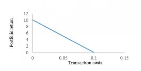
To remark the relationship of transaction costs and expected return, Figure 2 is drawn. The expected return and the transaction cost are represented in the vertical axis and the horizontal axis respectively. The expected return will decrease with the transaction costs levels increases, which is in conscience with intuitivity.
Figure 2. Behavior of return investment in function of transaction costs value using model 11
It is remarked also that, in the presence or absence of reality factors, the VaR will increase with the desired return levels increases. Figure 3 is drawn to see this point intuitively, in which the vertical axis is the expected return and the horizontal axis is the corresponding minimum Value at Risk.
Figure 3. Investment return of model 11
In this study, two Mean-Value at Risk (Mean-VaR) models for international portfolio optimization, grounded in uncertainty theory, are presented. To more accurately depict market realities, transaction costs and a desired level of portfolio diversification, as measured by the entropy measure, are incorporated into these models. A deterministic model is developed wherein security prices and exchange rate variables adhere to certain types of uncertainty distribution.
Compared to existing international portfolio optimization models in the literature, our model yields superior results in terms of diversification. It also reveals the impact of real-world constraints on optimal allocation and investment return. The model's validity was further corroborated through a numerical example, demonstrating that the optimal portfolio is more diversified when an entropy constraint is present. The model also suggests that returns could be relatively lower when no entropy constraint is considered. Moreover, expected returns are shown to decrease as the levels of transaction costs increase.
In conclusion, we outline several potential avenues for future research. Firstly, models incorporating additional real-world constraints, such as minimum transaction lots and bankruptcy within the investment horizon, could more accurately reflect the actual conditions of the securities market. Secondly, extending our model to accommodate multi-period cases and fractional optimization is another direction for further exploration. Finally, the use of metaheuristic algorithms to solve portfolio optimization problems could potentially enhance performance.
[1] Jondeau, E., Rockinger, M. (2006). Optimal portfolio allocation under higher moments. European Financial Management, 12(1): 29-55. http://doi.org/10.1111/j.1354-7798.2006.00309.x
[2] Kim, Y.S., Giacometti, R., Rachev, S.T., Fabozzi, F.J., Mignacca, D. (2012). Measuring financial risk and portfolio optimization with a non-Gaussian multivariate model. Annals of Operations Research, 201(1): 325-343. http://doi.org/10.1007/s10479-012-1229-8
[3] Konno, H., Yamazaki, H. (1991). Mean-absolute deviation portfolio optimization model and its applications to Tokyo stock market. Management Science, 37(5): 519-531. http://doi.org/10.1287/mnsc.37.5.519
[4] Patalay, S., Bandlamudi, M.R. (2021). Decision support system for stock portfolio selection using artificial intelligence and machine learning. Ingénierie des Systèmes d’Information, 26(1): 87-93. http://doi.org/10.18280/isi.260109
[5] Markowitz, H.M. (1952). Portfolio Selection. The Journal of Finance, 7(1): 77-91. http://doi.org/10.2307/2975974
[6] Markowitz, H.M. (1959). Portfolio Selection: Efficient Diversification of Investments. New Haven: Yale University Press. http://doi.org/10.12987/9780300191677
[7] Fishburn, P.C. (1977). Mean-risk analysis with risk associated with below-target returns. The American Economic Review, 67(2): 116-126.
[8] Lee, W.Y., Rao, R.K. (1988). Mean lower partial moment valuation and lognormally distributed returns. Management Science, 34(4): 446-453. https://doi.org/10.1287/mnsc.34.4.446
[9] Vercher, E., Bermudez, J.D., Segura, J.V. (2007). Fuzzy portfolio optimization under downside risk measures. Fuzzy Sets and Systems, 158(7): 769-782. https://doi.org/10.1016/j.fss.2006.10.026
[10] Butler, K.C., Joaquin, D.C. (2002). Are the gains from international portfolio diversification exaggerated? The influence of downside risk in bear markets. Journal of International Money and Finance, 21(7): 981-1011. https://doi.org/10.2139/ssrn.221992
[11] RiskMetrics. (1996). Technical Document. 4-th edition. JP Morgan Inc.
[12] Alexander, S., Coleman, T.F., Li, Y. (2006). Minimizing CVaR and VaR for a portfolio of derivatives. Journal of Banking & Finance, 30(2): 583-605. https://doi.org/10.1016/j.jbankfin.2005.04.012
[13] Wipplinger, E. (2007). Philippe Jorion: Value at risk-the new benchmark for managing financial risk. Financial Markets and Portfolio Management, 21(3): 397-398. http://doi.org/10.1007/s11408-007-0057-3
[14] Puelz, A.V. (2001). Value-at-risk based portfolio optimization. In Stochastic optimization: Algorithms and Applications (pp. 279-302). Springer, Boston, MA. https://doi.org/10.1007/978-1-4757-6594-6_13
[15] Hicks, J. (1980). Causality in Economics. Australian National University Press.
[16] Liu, D. (2007). Uncertainty theory. In Uncertainty Theory, Springer-Verlag Berlin Heidelberg 2015, pp. 205-234. http://doi.org/10.1007/978-3-662-44354-5
[17] Liu, B. (2010). Uncertainty theory. In Uncertainty Theory, Springer-Verlag Berlin Heidelberg 2015, pp. 1-79. http://doi.org/10.1007/978-3-662-44354-5
[18] Huang, X. (2012). Mean–variance models for portfolio selection subject to experts’ estimations. Expert Systems with Applications, 39(5): 5887-5893. https://doi.org/10.1016/j.eswa.2011.11.119
[19] Ning, Y., Yan, L., Xie, Y. (2013). Mean-TVaR model for portfolio selection with uncertain returns. International Information Institute (Tokyo). Information, 16(2): 977-985.
[20] Yin, M., Qian, W., Li, W. (2016). Portfolio selection models based on Cross-entropy of uncertain variables. Journal of Intelligent & Fuzzy Systems, 31(2): 737-747. http://doi.org/10.3233/JIFS-169006
[21] Liu, Y., Qin, Z. (2012). Mean semi-absolute deviation model for uncertain portfolio optimization problem. Journal of Uncertain Systems, 6(4): 299-307.
[22] Qin, Z., Kar, S., Zheng, H. (2016). Uncertain portfolio adjusting model using semiabsolute deviation. Soft Computing, 20(2): 717-725. https://doi.org/10.1007/s00500-014-1535-y
[23] Huang, X., Zhao, T. (2014). Mean-chance model for portfolio selection based on uncertain measure. Insurance: Mathematics and Economics, 59: 243-250. https://doi.org/10.1016/j.insmatheco.2014.10.001
[24] Zhai, J., Bai, M. (2017). Uncertain portfolio selection with background risk and liquidity constraint. Mathematical Problems in Engineering, 2017: 8249026. https://doi.org/10.1155/2017/8249026
[25] Zhang, Q., Huang, X., Zhang, C. (2015). A mean-risk index model for uncertain capital budgeting. Journal of the Operational Research Society, 66(5): 761-770. https://doi.org/10.1057/jors.2014.51
[26] Xue, L., Di, H., Zhao, X., Zhang, Z. (2019). Uncertain portfolio selection with mental accounts and realistic constraints. Journal of Computational and Applied Mathematics, 346: 42-52. https://doi.org/10.1016/j.cam.2018.06.049
[27] Bhattacharyya, R., Chatterjee, A., Kar, S. (2013). Uncertainty theory based multiple objective mean-entropy-skewness stock portfolio selection model with transaction costs. Journal of Uncertainty Analysis and Applications, 1(1): 1-17. https://doi.org/10.1186/2195-5468-1-16
[28] Lobo, M.S., Fazel, M., Boyd, S. (2007). Portfolio optimization with linear and fixed transaction costs. Annals of Operations Research, 152(1): 341-365. https://doi.org/10.1007/s10479-006-0145-1
[29] Arnott, R.D., Wagner, W.H. (1990). The measurement and control of trading costs. Financial Analysts Journal, 46(6): 73-80. https://doi.org/10.2469/faj.v46.n6.73
[30] Zhang, P. (2019). Multiperiod mean absolute deviation uncertain portfolio selection with real constraints. Soft Computing, 23: 5081-5098. https://doi.org/10.1007/s00500-018-3176-z
[31] Chen, W., Li, D., Lu, S., Liu, W. (2019). Multi-period mean–semivariance portfolio optimization based on uncertain measure. Soft Computing, 23: 6231-6247.
[32] Chen, L., Peng, J., Zhang, B., Rosyida, I. (2017). Diversified models for portfolio selection based on uncertain semivariance. International Journal of Systems Science, 48(3): 637-648. https://doi.org/10.1080/00207721.2016.1206985
[33] Jiang, C., Ma, Y., An, Y. (2013). International portfolio selection with exchange rate risk: A behavioural portfolio theory perspective. Journal of Banking & Finance, 37(2): 648-659. https://doi.org/10.1016/j.jbankfin.2012.10.004
[34] Gorman, L.R., Jorgensen, B. (2002). Domestic versus international portfolio selection: A statistical examination of the home bias. Multinational Finance Journal, 6(3/4): 131-166. https://doi.org/10.17578/6-3/4-1
[35] Huang, X. (2010). Mean-variance Zadehmodels for international portfolio selection with uncertain exchange rates and security returns. In 2010 International Conference on Information Science and Applications, Seoul, Korea (South), pp. 1-7. https://doi.org/10.1109/icisa.2010.5480377
[36] Huang, X., Wang, X. (2021). International portfolio optimization based on uncertainty theory. Optimization, 70(2): 225-249. https://doi.org/10.1080/02331934.2019.1705821
[37] Wang, X., Gao, Z., Guo, H. (2012). Delphi method for estimating uncertainty distributions. Information: An International Interdisciplinary Journal, 15(2): 449-460.
[38] Zadeh, L.A. (1965). Fuzzy sets. Information and Control, 8(3): 338-353. https://doi.org/10.1016/s0019-9958(65)90241-x
[39] Li, X., Qin, Z., Kar, S. (2010). Mean-variance-skewness model for portfolio selection with fuzzy returns. European Journal of Operational Research, 202(1): 239-247. https://doi.org/10.1016/j.ejor.2009.05.003
[40] Carlsson, C., Fullér, R., Majlender, P. (2002). A possibilistic approach to selecting portfolios with highest utility score. Fuzzy Sets and Systems, 131(1): 13-21. https://doi.org/10.1016/s0165-0114(01)00251-2
[41] Huang, X. (2008). Mean-semivariance models for fuzzy portfolio selection. Journal of computational and applied mathematics, 217(1): 1-8. https://doi.org/10.1016/j.cam.2007.06.009
[42] Peng, Z., Iwamura, K. (2010). A sufficient and necessary condition of uncertainty distribution. Journal of Interdisciplinary Mathematics, 13(3): 277-285. https://doi.org/10.1080/09720502.2010.10700701
[43] Peng, J. (2013). Risk metrics of loss function for uncertain system. Fuzzy Optimization and Decision Making, 12(1): 53-64. https://doi.org/10.1007/s10700-012-9146-5
[44] Mansini, R., Ogryczak, W., Speranza, M.G. (2014). Twenty years of linear programming based portfolio optimization. European Journal of Operational Research, 234(2): 518-535. https://doi.org/10.1016/j.ejor.2013.08.035
[45] Berry, C.H. (2015). Corporate Growth and Diversification. Princeton University Press. https://doi.org/10.1515/9781400872961
[46] Shannon, C.E., Weaver, W. (1949). The mathematical theory of information. Urbana: University of Illinois Press, 97(6): 128-164.
[47] Palepu, K. (1985). Diversification strategy, profit performance and the entropy measure. Strategic Management Journal, 6(3): 239-255. https://doi.org/239-255. https://doi.org/10.1002/smj.4250060305