Rasha H. Ibraheem![]() | Rawaa I. Esa
| Rawaa I. Esa![]() | Ali F. Jameel*
| Ali F. Jameel*![]()
© 2023 IIETA. This article is published by IIETA and is licensed under the CC BY 4.0 license (http://creativecommons.org/licenses/by/4.0/).
OPEN ACCESS
This study presents a novel computational methodology for resolving second-order fuzzy initial value problems (FIVPs), encompassing ordinary differential equations. The proposed approach modifies the conventional crisp fifth-order Runge-Kutta Fehlberg method to suit the resolution of second-order FIVPs within the fuzzy domain, drawing on concepts from fuzzy set theory. It is demonstrated that by reducing them to a system of first-order FIVPs, all second-order FIVPs can be effectively solved. The novel method is subsequently applied to both linear and non-linear second-order FIVPs. The results attest to the high efficiency and accuracy of the approach, while also preserving the inherent properties of fuzzy solutions. Therefore, this study offers a promising new avenue for addressing second-order FIVPs, with potential applicability across a broad range of scenarios.
fuzzy sets theory, fuzzy differential equation, second order FIVPs, fifth order Range -Kutta Fehlberg method (RKF5)
Various intricate real-world problems can be formulated as conceptual models, which can be articulated through ordinary or partial differential equations [1, 2]. Multiple numerical methods can be employed to resolve these differential equations across diverse domains [3-7]. Fuzzy initial value problems (FIVPs) emerge when such models are not fully developed and exhibit unpredictability. These models, characterized by uncertainty, can be represented as fuzzy differential equations (FDEs), which are mathematical dynamic systems models. FDEs are increasingly being applied to tackle real-world problems in fields such as biological models, physics applications, and medical sciences [8-11].
The discipline of numerical analysis, an intersection of mathematics and computer science, is pivotal in devising, analyzing, and implementing methods for numerically solving varying mathematical problems. Despite the potential of numerical approaches to handle complex problems, the extent of computing power invariably imposes limitations. For instance, to address certain problems, the application of numerical methods becomes indispensable.
Two prevalent methods of resolving FIVPs are analytical and numerical approaches. The analytical methodology furnishes a closed-form solution, often referred to as the exact solution [12]. The solution may be assembled from a limited set of basic functions, such as polynomials, exponentials, trigonometric, and hyperbolic functions. The advantage of an exact solution is that it offers a comprehensive understanding of the problem solution, thus, it does not always necessitate extensive computation to interpret the findings [13].
However, certain mathematical models, especially FDEs, pose challenges in procuring analytical solutions. Consequently, numerical methods may be required to evaluate solutions to physical problems. Although employing analogous methods to solve these equations offers benefits, it also presents inherent limitations. There is a pressing need for more research into superior numerical methodologies for FDEs, the effectiveness of which has yet to be scrutinized using their results.
The efficacy of the presented technique can be assessed on linear FIVPs, which is one of the most apparent factors. The stability of the Runge Kutta methods in solving such problems relies on the increment of calculations in the method function per step [14]. Recent studies have utilized fourth-order Runge-Kutta methods to evaluate the numerical solution of linear FIVPs [15, 16], and enhanced Runge-Kutta Nystrom methods of varying orders to solve pairs of FIVPs in linear forms [17].
Modifications of the standard fifth-order range Kutta method from the crisp domain to the fuzzy domain have been used to solve second-order linear and nonlinear FIVPs [18, 19]. In addition, the polynomial form of second-order linear FIVPs has been obtained via the undetermined fuzzy coefficients method (UFCM) [20]. However, the Runge-Kutta Fehlberg fifth-order method (RKF5) has not yet been applied to second-order linear and nonlinear FIVPs. It would, therefore, be intriguing to examine the numerical solution and analysis of RKF5 on various second-order FDEs involving linear and nonlinear FIVPs.
The present study, therefore, concentrates on the numerical solution of second-order FIVPs and aims to demonstrate its proficiency in terms of accuracy compared with some methods from the preceding survey. To the authors' best knowledge, no research has extended the general form of the crisp RKF5 domain to the fuzzy domain to devise a novel form for solving such class of FDEs.
We will discuss the fundamental terms and definitions related to fuzzy sets theory in this section, which will make it easier for us to understand the work in the following sections, such as the fuzzy fractional numbers, which are a generalization of the traditional crisp number [20-23]. It is important to note that the FDEs also employ the idea of fuzzy leve sets. The α-cut or fuzzy level sets are fuzzy numbers that convert the whole fuzzy system to crisp system with more genralzation transforms an imprecise data into precise data this called defuzzification [21]. On the other hand, it's important to remember the following basic concept of fuzzy sets:
Definition 2.2 [20]: $\tilde{\mathrm{f}}(\mathrm{x})$ is a fuzzy function if $\mathrm{f}: \mathbb{R} \rightarrow \widetilde{\mathrm{E}}$, where, if $\widetilde{E}$ be the set of all fuzzy numbers.
Definition 2.3 [20]: $\mathrm{f}: \mathrm{K} \rightarrow \widetilde{\mathrm{E}}$ called a fuzzy function process on interval $K \subseteq \widetilde{\mathrm{E}}$, then the $\alpha$-level set is:
$[\tilde{\mathrm{f}}(\mathrm{x})]_\alpha=[\underline{\mathrm{f}}(\mathrm{x} ; \alpha), \overline{\mathrm{f}}(\mathrm{x} ; \alpha)], \mathrm{x} \in \mathrm{K}, \alpha \in[0,1]$.
Using the α-level sets, we can characterize and describe fuzzy sets more effectively. They provide a comprehensive view of the fuzzy set's membership distribution, allowing us to observe the gradual change in membership grades. Moreover, α-level sets enable comparisons and analysis between different fuzzy sets based on their overlapping or containment relationships at different levels of resolution.
Definition 2.5 [24]: Each function $f: X \rightarrow Y$ induces another function $\tilde{f}: F(X) \rightarrow F(Y)$ defined for each fuzzy interval $\mathrm{U}$ in $\mathrm{X}$ by:
$\tilde{f}(\mathrm{U})(v)= \begin{cases}\operatorname{Sup}_{\mathrm{x} \in \mathrm{f}^{-1}(\mathrm{y})} \mathrm{U}(\mathrm{x}) & , \text { if } v \in \operatorname{range}(\mathrm{f}) \\ 0 & , \text { if } v \notin \operatorname{range}(\mathrm{f})\end{cases}$
This is called the Zadeh extension principle.
Definition 2.6 [25]: Consider $\widetilde{x}, \widetilde{v} \in \widetilde{E}$. If there exists $\widetilde{z} \in \widetilde{E}$ such that $\widetilde{x}=\widetilde{v}+\widetilde{z}$, then $\widetilde{z}$ is called the H-difference (Hukuhara difference) of $\mathrm{x}$ and $\mathrm{y}$ and is denoted by $\widetilde{z}=\widetilde{x} \ominus \widetilde{v}$.
Definition 2.7 [20]: If $\tilde{\mathrm{f}}: \mathrm{I} \rightarrow \widetilde{\mathrm{E}}$ and $\mathrm{y}_0 \in \mathrm{I}$, where $\mathrm{I} \in\left[\mathrm{x}_0, \mathrm{~K}\right]$. We say that $\tilde{f}$ Hukuhara differentiable at $y_0$, if there exists an element $\left[\tilde{\mathrm{f}}^{\prime}\right]_\alpha \in \widetilde{\mathrm{E}}$ such that for all $\mathrm{h}>0$ sufficiently small (near to 0$)$, exists $\tilde{\mathrm{f}}\left(v_0+\mathrm{h} ; \alpha\right) \ominus \tilde{\mathrm{f}}\left(v_0 ; \alpha\right), \tilde{\mathrm{f}}\left(v_0 ; \alpha\right) \ominus \tilde{\mathrm{f}}\left(\mathrm{y}_0-\mathrm{h} ; \alpha\right)$ and the limits are taken in the metric $(\widetilde{\mathrm{E}}, \mathrm{D})$:
$\lim _{\mathrm{h} \rightarrow 0+} \frac{\tilde{\mathrm{f}}\left(v_0+\mathrm{h} ; \alpha\right) \ominus \tilde{\mathrm{f}}\left(\mathrm{y}_0 ; \alpha\right)}{\mathrm{h}}=\lim _{\mathrm{h} \rightarrow 0+} \frac{\tilde{\mathrm{f}}\left(v_0 ; \alpha\right) \ominus \tilde{\mathrm{f}}\left(v_0-\mathrm{h} ; \alpha\right)}{\mathrm{h}}$
The fuzzy set $\left[\widetilde{\mathrm{f}}^{\prime}\left(v_0\right)\right]_\alpha$ is called the Hukuhara derivative of $\left[\tilde{\mathrm{f}}^{\prime}\right]_\alpha$ at $v_0$.
These limits are taken in the space $(\widetilde{\mathrm{E}}, \mathrm{D})$ if $\mathrm{x}_0$ or $\mathrm{K}$, then we consider the corresponding one-side derivation. Recall that $\tilde{\mathrm{x}} \Theta \tilde{v}=\tilde{\mathrm{z}} \in \widetilde{\mathrm{E}}$ are defined on $\alpha$-level set, where $[\tilde{\mathrm{x}}]_\alpha \ominus[\tilde{v}]_\alpha=[\tilde{\mathrm{z}}]_\alpha, \forall \alpha \in[0,1]$. By consideration of definition of the metric D all the r-level set $[\tilde{\mathrm{f}}(0)]_\alpha$ are Hukuhara differentiable at $y_0$, with Hukuhara derivatives $\left[\widetilde{\mathrm{f}^{\prime}}\left(v_0\right)\right]_\alpha$, when $\tilde{\mathrm{f}}: \mathrm{I} \rightarrow \widetilde{\mathrm{E}}$ is Hukuhara differentiable at $y_0$ with Hukuhara derivative $\left[\widetilde{\mathrm{f}^{\prime}}\left(v_0\right)\right]_\alpha$ it' lead to that $\tilde{\mathrm{f}}$ is Hukuhara differentiable for all $\alpha \in[0,1]$ which satisfies the above limits i.e. if $\mathrm{f}$ is differentiable at $\mathrm{x}_0 \in\left[\mathrm{x}_0+\alpha, \mathrm{K}\right]$ then all its $\alpha$-levels $\left[\tilde{\mathrm{f}}^{\prime}(\mathrm{x})\right]_\alpha$ are Hukuhara differentiable at $\mathrm{x}_0$.
Definition 2.8 [20]: Define the mapping $\widetilde{\mathrm{f}^{\prime}}: \mathrm{I} \rightarrow \widetilde{\mathrm{E}}$ and $\mathrm{y}_0 \in \mathrm{I}$, where $\mathrm{I} \in\left[\mathrm{x}_0, \mathrm{~K}\right]$. We say that $\widetilde{\mathrm{f}^{\prime}}$ Hukuhara differentiable $\mathrm{x} \in \widetilde{\mathrm{E}}$, if there exists an element $\left[\tilde{\mathrm{f}}^{(\mathrm{n})}\right]_\alpha \in \widetilde{\mathrm{E}}$ such that for all $\mathrm{h}>0$ sufficiently small (near to 0$)$, exists $\tilde{\mathrm{f}}^{(\mathrm{n}-1)}\left(v_0+\mathrm{h} ; \alpha\right) \ominus \tilde{\mathrm{f}}^{(\mathrm{n}-1)}\left(v_0 ; \alpha\right), \tilde{\mathrm{f}}^{(\mathrm{n}-1)}\left(v_0 ; \alpha\right) \ominus \tilde{\mathrm{f}}^{(\mathrm{n}-1)}\left(v_0-\mathrm{h} ; \alpha\right)$ and the limits are taken in the metric $(\widetilde{\mathrm{E}}, \mathrm{D})$.
$\lim _{\mathrm{h} \rightarrow 0+} \frac{\tilde{\mathrm{f}}^{(\mathrm{n}-1)}\left(v_0+\mathrm{h} ; \alpha\right) \Theta \tilde{\mathrm{f}}^{(\mathrm{n}-1)}\left(v_0 ; \alpha\right)}{\mathrm{h}}=\lim _{\mathrm{h} \rightarrow 0+} \frac{\tilde{\mathrm{f}}^{(\mathrm{n}-1)}\left(v_0 ; \alpha\right) \Theta \tilde{\mathrm{f}}^{(\mathrm{n}-1)}\left(v_0-\mathrm{h} ; \alpha\right)}{\mathrm{h}}$
exists and equal to $\tilde{\mathrm{f}}^{(\mathrm{n})}$ and for $\mathrm{n}=2$, we have second order Hukuhara derivative.
Theorem 2.2 [20]: Let $\tilde{\mathrm{f}}:\left[\mathrm{x}_0+\alpha, \mathrm{K}\right] \rightarrow \widetilde{\mathrm{E}}$ be Hukuhara differentiable and denote.
$\left[\widetilde{\mathrm{f}}^{\prime}(\mathrm{x})\right]_\alpha=\left[\underline{\mathrm{f}}^{\prime}(\mathrm{x}), \overline{\mathrm{f}}^{\prime}(\mathrm{x})\right]_\alpha=\left[\underline{\mathrm{f}}^{\prime}(\mathrm{x} ; \alpha), \overline{\mathrm{f}}^{\prime}(\mathrm{x} ; \alpha)\right]$.
Then the boundary functions $\underline{f}^{\prime}(x ; \alpha), \bar{f}^{\prime(x ; \alpha)}$ are differentiable we can write for second order fuzzy derivative:
$\left[\tilde{\mathrm{f}}^{\prime \prime}(\mathrm{x})\right]_\alpha=\left[\left(\underline{\mathrm{f}}^{\prime \prime}(\mathrm{x} ; \alpha)\right)^{\prime},\left(\overline{\mathrm{f}}^{\prime \prime}(\mathrm{x} ; \alpha)\right)^{\prime}\right], \forall \alpha \in[0,1]$.
The following is an ordinary differential equation with second-order fuzzy initial values:
$\left\{\begin{array}{c}\frac{\mathrm{d}^2 \tilde{v}(\mathrm{x} ; \alpha)}{\mathrm{dx}^2}=\tilde{\mathrm{f}}\left(\mathrm{x}, \tilde{\mathrm{v}}(\mathrm{x} ; \alpha), \frac{\mathrm{d} \tilde{\mathrm{v}}(\mathrm{x} ; \alpha)}{\mathrm{dx}}\right)+\tilde{\mathrm{u}}(\mathrm{x} ; \alpha) \\ \tilde{v}\left(\mathrm{x}_0 ; \alpha\right)=(\tilde{\mathrm{a}})_\alpha, \tilde{v}^{\prime}\left(\mathrm{x}_0 ; \alpha\right)=(\tilde{\mathrm{b}})_\alpha \\ \mathrm{x} \in\left[\mathrm{x}_0, \mathrm{X}\right], \alpha \in[0,1],\end{array}\right.$ (1)
where, $\frac{\mathrm{d}^2 \tilde{v}(\mathrm{x} ; \alpha)}{\mathrm{dx}^2}$ denoted as a second order fuzzy H-derivative, $\tilde{\mathrm{f}}$ is the function of the crisp variable $\mathrm{x}$ that take the values between starting point $\mathrm{x}_0$ and end point $\mathrm{X}$. The fuzzy function $\tilde{v}(x ; \alpha)$ and the first order fuzzy H-derivative $\frac{\mathrm{d} \tilde{v}(\mathrm{x} ; \alpha)}{\mathrm{dx}}$. Also, in Eq. (1) the nonhomogeneous term is refer to fuzzy function $\tilde{\mathrm{u}}(\mathrm{x} ; \alpha)$. The initial conditions $\tilde{v}^{\prime}\left(\mathrm{x}_0 ; \alpha\right)$ and $\tilde{v}^{\prime}\left(\mathrm{x}_0 ; \alpha\right)$ that equal to $(\tilde{\mathrm{a}})_\alpha$ and $(\tilde{\mathrm{b}})_\alpha$ respectively are fuzzy numbers. From the fuzzy analysis in studies [18, 19], Eq. (1) can be reduced to two fuzzy first-order differential equations as follows:
$\left\{\begin{array}{l}\frac{\mathrm{d} \tilde{v}(\mathrm{x} ; \alpha)}{\mathrm{dx}}=\tilde{\mathrm{f}}(\mathrm{x}, \tilde{v}(\mathrm{x} ; \alpha), \tilde{\mathrm{z}}(\mathrm{x} ; \alpha)), \mathrm{x} \in\left[\mathrm{x}_0, \mathrm{X}\right] \\ \frac{\mathrm{d} \tilde{\mathrm{z}}(\mathrm{x} ; \alpha)}{\mathrm{dx}}=\tilde{\mathrm{g}}(\mathrm{x}, \tilde{v}(\mathrm{x} ; \alpha), \tilde{\mathrm{z}}(\mathrm{x} ; \alpha)), \\ \tilde{v}\left(\mathrm{x}_0 ; \alpha\right)=(\tilde{\mathrm{a}})_\alpha,=\tilde{\mathrm{z}}\left(\mathrm{x}_0 ; \alpha\right)=(\tilde{\mathrm{b}})_\alpha,\end{array}\right.$ (2)
where, $\frac{\mathrm{d} \tilde{v}(\mathrm{x} ; \alpha)}{\mathrm{dx}}$ and $\frac{\mathrm{d} \tilde{\mathrm{z}}(\mathrm{x} ; \alpha)}{\mathrm{dx}}$ are first order fuzzy H-derivative of the fuzzy functions $\tilde{v}(\mathrm{x} ; \alpha)$ and $\tilde{z}(x ; \alpha)$. Here in Eq. (2) the fuzzy function:
$\begin{gathered}\tilde{\mathrm{f}}(\mathrm{x}, \tilde{\mathrm{v}}(\mathrm{x} ; \alpha), \tilde{\mathrm{z}}(\mathrm{x} ; \alpha))=\tilde{\mathrm{z}}(\mathrm{x} ; \alpha)+\tilde{\mathrm{u}}(\mathrm{x} ; \alpha) \\ \tilde{\mathrm{z}}(\mathrm{x} ; \alpha)=v^{\prime}(\mathrm{x} ; \alpha)\end{gathered}$
$\mathrm{g}(\mathrm{x}, \tilde{\mathrm{v}}(\mathrm{x} ; \alpha), \tilde{\mathrm{z}}(\mathrm{x} ; \alpha))$ is a fuzzy function of the crips variable $\mathrm{x}$ and the fuzzy unctions $\tilde{v}(\mathrm{x} ; \alpha)$ and $\tilde{\mathrm{z}}(\mathrm{x} ; \alpha)$ and the fuzzy numbers $\tilde{v}\left(\mathrm{x}_0 ; \alpha\right)$ and $\tilde{\mathrm{z}}\left(\mathrm{x}_0 ; \alpha\right)$ are the initial conditions. For all $\alpha \in[0,1]$ the defuzzification of Eq. (2) is giving as below:
$\begin{aligned} & {[\tilde{v}(\mathrm{x})]_\alpha=[\underline{v}(\mathrm{x}, \alpha), \bar{v}(\mathrm{x}, \alpha)],[\tilde{\mathrm{z}}(\mathrm{x})]_\alpha=[\underline{\mathrm{z}}(\mathrm{x}, \alpha), \overline{\mathrm{z}}(\mathrm{x}, \alpha)]} \\ & {[\tilde{\mathrm{f}}(\mathrm{x}, \tilde{v}(\mathrm{x}), \tilde{\mathrm{z}}(\mathrm{x}))]_\alpha=[\underline{\mathrm{f}}(\mathrm{x}, \tilde{v}(\mathrm{x}), \tilde{\mathrm{z}}(\mathrm{x})), \overline{\mathrm{f}}(\mathrm{x}, \tilde{v}(\mathrm{x}), \tilde{\mathrm{z}}(\mathrm{x}))]_\alpha} \\ & {[\tilde{\mathrm{g}}(\mathrm{x}, \tilde{v}(\mathrm{x}), \tilde{\mathrm{z}}(\mathrm{x}))]_\alpha=[\underline{\mathrm{g}}(\mathrm{x}, \tilde{v}(\mathrm{x}), \tilde{\mathrm{z}}(\mathrm{x})), \overline{\mathrm{f}}(\mathrm{x}, \tilde{v}(\mathrm{x}), \tilde{\mathrm{z}}(\mathrm{x}))]_\alpha}\end{aligned}$
For simplicity, assume that.
$\begin{gathered}\tilde{\mathrm{f}}(\mathrm{x}, \tilde{\mathrm{v}}, \tilde{\mathrm{z}} ; \alpha)=[\underline{\mathrm{f}}(\mathrm{x}, \tilde{\mathrm{v}}, \tilde{\mathrm{z}}), \overline{\mathrm{f}}(\mathrm{x}, \tilde{\mathrm{v}}, \tilde{\mathrm{z}})]_\alpha \\ \tilde{\mathrm{g}}(\mathrm{x}, \tilde{\mathrm{v}}, \tilde{\mathrm{z}} ; \alpha)=[\underline{\mathrm{g}}(\mathrm{x}, \tilde{\mathrm{v}}, \tilde{\mathrm{z}}), \overline{\mathrm{g}}(\mathrm{x}, \tilde{\mathrm{v}}, \tilde{\mathrm{z}})]_\alpha \\ \underline{\mathrm{z}}(\mathrm{x} ; \alpha)=\underline{\mathrm{z}}(\mathrm{x}, \tilde{\mathrm{v}}, \tilde{\mathrm{z}} ; \alpha)=\mathrm{F}(\mathrm{x}, \underline{v}, \overline{\mathrm{v}}, \underline{\mathrm{z}}, \overline{\mathrm{z}} ; \alpha) \\ \overline{\mathrm{z}}(\mathrm{x} ; \alpha)=\overline{\mathrm{z}}(\mathrm{x}, \tilde{\mathrm{v}}, \tilde{\mathrm{z}} ; \alpha)=\mathrm{G}(\mathrm{x}, \underline{\mathrm{v}}, \overline{\mathrm{v}}, \underline{\mathrm{z}}, \overline{\mathrm{z}} ; \alpha) \\ {\left[\tilde{\mathrm{v}}\left(\mathrm{x}_0\right)\right]_\alpha=\left[\underline{\mathrm{v}}\left(\mathrm{x}_0 ; \alpha\right), \overline{\mathrm{v}}\left(\mathrm{x}_0 ; \alpha\right)\right],\left[\tilde{v}_0\right]_\alpha=\left[\underline{v_0}, \overline{v_0}\right]_\alpha=[\underline{\mathrm{a}}, \overline{\mathrm{a}}]_\alpha} \\ {\left[\tilde{\mathrm{z}}\left(\mathrm{x}_0\right)\right]_\alpha=\left[\underline{\mathrm{z}}\left(\mathrm{x}_0 ; \alpha\right), \overline{\mathrm{z}}\left(\mathrm{x}_0 ; \alpha\right)\right],\left[\tilde{\mathrm{z}}_0\right]_\alpha=\left[\underline{\mathrm{z}_0}, \overline{\mathrm{z}_0}\right]_\alpha=[\underline{\mathrm{b}}, \overline{\mathrm{b}}]_\alpha}\end{gathered}$
The next membership function is created by applying the extension principle:
$\begin{aligned} \tilde{\mathrm{f}}(\mathrm{x}, \tilde{v}, \tilde{\mathrm{z}} ; \alpha)(\mathrm{s}) & =\sup \{(\tilde{v}, \tilde{\mathrm{z}})(\tau) \mid \mathrm{s}=\tilde{\mathrm{f}}(\mathrm{x}, \tau)\}, \mathrm{s} \in \mathrm{R} \\ \tilde{\mathrm{g}}(\mathrm{x}, \tilde{v}, \tilde{\mathrm{z}} ; \alpha)(\mathrm{s}) & =\sup \{(\tilde{v}, \tilde{\mathrm{z}})(\tau) \mid \mathrm{s}=\tilde{\mathrm{g}}(\mathrm{x}, \tau)\}, \mathrm{s} \in \mathrm{R}\end{aligned}$
where,
$\begin{aligned} & \underline{\mathrm{f}}(\mathrm{x}, \tilde{\mathrm{v}}, \tilde{\mathrm{z}} ; \alpha)=\min \{\tilde{\mathrm{f}}(\mathrm{x}, \tilde{\mathrm{v}}, \tilde{\mathrm{z}} ; \alpha) \mid\} \\ & \overline{\mathrm{f}}(\mathrm{x}, \tilde{v}, \tilde{\mathrm{z}} ; \alpha)=\max \{\tilde{\mathrm{f}}(\mathrm{x}, \tilde{\mathrm{v}}, \tilde{\mathrm{z}} ; \alpha) \mid\} \\ & \underline{\mathrm{g}}(\mathrm{x}, \tilde{\mathrm{v}}, \tilde{\mathrm{z}} ; \alpha)=\min \{\tilde{\mathrm{g}}(\mathrm{x}, \tilde{v}, \tilde{\mathrm{z}} ; \alpha) \mid\} \\ & \overline{\mathrm{g}}(\mathrm{x}, \tilde{v}, \tilde{\mathrm{z}} ; \alpha)=\max \{\tilde{\mathrm{g}}(\mathrm{x}, \tilde{v}, \tilde{\mathrm{z}} ; \alpha) \mid\}\end{aligned}$
Consider the exact solution of Eq. (2) that can define by:
$\left[\widetilde{\mathrm{V}}\left(\mathrm{x}_{\mathrm{n}}\right)\right]_\alpha=\left[\underline{\mathrm{V}}\left(\mathrm{x}_{\mathrm{n}} ; \alpha\right), \overline{\mathrm{V}}\left(\mathrm{x}_{\mathrm{n}} ; \alpha\right)\right]$
while the numerical solution defines as:
$\left[\tilde{v}\left(x_n\right)\right]_\alpha=\left[\underline{v}\left(x_n ; \alpha\right), \bar{v}\left(x_n ; \alpha\right)\right]$
By iteratively applying the RKF5 formulas, RKF5 is an explicit method which calculates the approximate solution to the ODE at the desired future time. It adjusts the step size dynamically based on error estimates to maintain accuracy while minimizing computational effort. The method provides an efficient and reliable approach to numerically solve ODEs, particularly those with smooth solutions [26-28]. The basis of all Runge-Kutta methods in is to express the difference between the value of $\left[\tilde{y}\left(x_n\right)\right]_\alpha$ at $x_{n+1}$ and $x_n$ as in such that for each $\alpha \in[0,1]$:
$\tilde{y}_{n+1}\left(x_{n+1} ; \alpha\right)-\tilde{y}_n\left(x_n ; \alpha\right)=\sum_{i=1}^N c_n k_n$ (3)
where, for n=0,1, 2..., N the cn are the constants and:
$\mathrm{k}_{\mathrm{i}}=\mathrm{f}\left(\mathrm{x}_{\mathrm{n}}+\mathrm{h} \mathrm{r}_{\mathrm{n}}, \tilde{\mathrm{y}}\left(\mathrm{x}_{\mathrm{n}} ; \tilde{\mathrm{y}}_{\mathrm{n}}\left(\mathrm{x}_{\mathrm{n}} ; \alpha\right)\right)+\mathrm{h} \sum_{\mathrm{j}=1}^{\mathrm{s}-1} \gamma_{\mathrm{js}} \mathrm{k}_{\mathrm{i}}\right)$ (4)
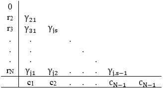
To specify a particular method, one needs to provide the integer N (the number of stages), and the coefficients γjn, cn and rn (for n, j = 1, 2..., N). The matrix [γjn] is called the Runge–Kutta matrix, while the cn and rn are known as the weights and the nodes [14]. These data are usually arranged in a mnemonic device, known as a Butcher tableau [29]:
Eq. (2) is to be exact for powers of h through hp, where p is the order of the Runge-Kutta methods, because it is to be coincident with Taylor series of order p [29]. Therefore from [14], the truncation error TN in of order p+1 can be written:
$\mathrm{T}_{\mathrm{N}}=\delta_{\mathrm{N}} \mathrm{h}^{\mathrm{p}+1}+\mathrm{O}\left(\mathrm{h}^{\mathrm{p}+2}\right)$ (5)
where, the value of $\delta_{\mathrm{N}}$ will generally be much less than the bound. The nonzero constants $r_n, \gamma_{j n}$ in RKF5 given in the study [30] as $r_1=0, r_2=\frac{1}{4}, r_3=\frac{3}{8}, r_4=\frac{12}{13}, r_5=1, r_6=\frac{1}{2}$ and $\gamma_{21}=\frac{1}{4}, \gamma_{31}=\frac{3}{32}, \gamma_{41}=\frac{3}{16}, \gamma_{51}=\frac{439}{216}, \gamma_{61}=-\frac{8}{27}, \gamma_{32}=\frac{9}{32}, \gamma_{42}=$ $-\frac{7200}{2197}, \gamma_{43}=\frac{7296}{2197}, \gamma_{52}=-8, \gamma_{53}=\frac{3680}{513}, \gamma_{54}=-\frac{845}{4104}, \gamma_{62}=2, \gamma_{63}=-\frac{3544}{2565}, \gamma_{64}=\frac{1859}{4104}, \gamma_{64}=\frac{-11}{40}, c_1=\frac{16}{135}, c_2=0, c_3=$ $\frac{6656}{12825}, c_4=\frac{28561}{56430}, c_5=\frac{-9}{50}, c_6=\frac{2}{55}$, hence:
$\tilde{v}_{\mathrm{n}+1}\left(\mathrm{x}_{\mathrm{n}+1} ; \alpha\right)=\tilde{v}_{\mathrm{n}}\left(\mathrm{x}_{\mathrm{n}} ; \alpha\right)+\frac{16}{135} k_1+\frac{6656}{12825} k_3+\frac{28561}{56430} k_4-\frac{9}{50} k_5+\frac{2}{55} k_6$ (6)
where,
$\begin{gathered}\mathrm{k}_1=\mathrm{hf}\left(\mathrm{x}_{\mathrm{n}}, \tilde{v}_{\mathrm{n}}\left(\mathrm{x}_{\mathrm{n}} ; \alpha\right)\right), \\ \mathrm{k}_2=\mathrm{hf}\left(\mathrm{x}_{\mathrm{n}}+\frac{\mathrm{h}}{4}, \tilde{v}_{\mathrm{n}}\left(\mathrm{x}_{\mathrm{n}} ; \alpha\right)+\frac{\mathrm{k}_1}{4}\right), \\ \mathrm{k}_3=\mathrm{hf}\left(\mathrm{x}_{\mathrm{n}}+\frac{3 \mathrm{~h}}{8}, \tilde{v}_{\mathrm{n}}\left(\mathrm{x}_{\mathrm{n}} ; \alpha\right)+\frac{3 \mathrm{k}_1}{32}+\frac{9 \mathrm{k}_2}{32}\right), \\ \mathrm{k}_4=\mathrm{hf}\left(\mathrm{x}_{\mathrm{n}}+\frac{\mathrm{h}}{2}, \tilde{v}_{\mathrm{n}}\left(\mathrm{x}_{\mathrm{n}} ; \alpha\right)+\frac{1932 \mathrm{k}_1}{2197}-\frac{7002 \mathrm{k}_2}{2197}+\frac{7296 \mathrm{k}_3}{2197}\right), \\ \mathrm{k}_5=\mathrm{hf}\left(\mathrm{x}_{\mathrm{n}}+\frac{3 \mathrm{~h}}{4}, \tilde{v}_{\mathrm{n}}\left(\mathrm{x}_{\mathrm{n}} ; \alpha\right)+\frac{439 \mathrm{k}_1}{216}-8 \mathrm{k}_2+\frac{3680 \mathrm{k}_3}{513}+\frac{845 \mathrm{k}_4}{4104}\right), \\ \mathrm{k}_6=\mathrm{hf}\left(\mathrm{x}_{\mathrm{n}}+\mathrm{h}, \tilde{v}_{\mathrm{n}}\left(\mathrm{x}_{\mathrm{n}} ; \alpha\right)+\frac{8 \mathrm{k}_1}{27}+2 \mathrm{k}_2-\frac{3544 \mathrm{k}_3}{2565}+\frac{1859 \mathrm{k}_4}{4104}-\frac{11 \mathrm{k}_4}{40}\right) .\end{gathered}$
To solve Eq. (2) in linear and nonlinear forms numerically the new from RKF5 is obtained from the following fuzzy analysis as below:
$\begin{aligned} & v\left(\mathrm{x}_{\mathrm{n}+1}, \alpha\right)=\underline{v}\left(\mathrm{x}_{\mathrm{n}}, \alpha\right)+\mathrm{h} \sum_{\mathrm{j}=1}^6 \mathrm{w}_{\mathrm{j}} \underline{\mathrm{k}}_{\mathrm{j}, 1}\left(\mathrm{x}_{\mathrm{n}}, \tilde{\mathrm{y}}\left(\mathrm{x}_{\mathrm{n}} ; \alpha\right), \tilde{\mathrm{z}}\left(\mathrm{x}_{\mathrm{n}} ; \alpha\right)\right), \\ & \overline{\mathrm{y}}\left(\mathrm{x}_{\mathrm{n}+1}, \alpha\right)=\bar{v}\left(\mathrm{x}_{\mathrm{n}}, \alpha\right)+\mathrm{h} \sum_{\mathrm{j}=1}^6 \mathrm{w}_{\mathrm{j}} \overline{\mathrm{k}}_{\mathrm{j}, 2}\left(\mathrm{x}_{\mathrm{n}}, \tilde{v}\left(\mathrm{x}_{\mathrm{n}} ; \alpha\right), \tilde{\mathrm{z}}\left(\mathrm{x}_{\mathrm{n}} ; \alpha\right)\right), \\ & \underline{\mathrm{z}}\left(\mathrm{x}_{\mathrm{n}+1}, \alpha\right)=\underline{\mathrm{z}}\left(\mathrm{x}_{\mathrm{n}}, \alpha\right)+\mathrm{h} \sum_{\mathrm{j}=1}^6 \mathrm{w}_{\mathrm{j}} \underline{\mathrm{L}}_{\mathrm{j}, 1}\left(\mathrm{x}_{\mathrm{n}}, \tilde{v}\left(\mathrm{x}_{\mathrm{n}} ; \alpha\right), \tilde{\mathrm{z}}\left(\mathrm{x}_{\mathrm{n}} ; \alpha\right)\right), \\ & \overline{\mathrm{z}}\left(\mathrm{x}_{\mathrm{n}+1}, \alpha\right)=\overline{\mathrm{z}}\left(\mathrm{x}_{\mathrm{n}}, \alpha\right)+\mathrm{h} \sum_{\mathrm{j}=1}^6 \mathrm{w}_{\mathrm{j}} \overline{\mathrm{L}}_{\mathrm{j}, 2}\left(\mathrm{x}_{\mathrm{n}}, \bar{v}\left(\mathrm{x}_{\mathrm{n}}, \alpha\right), \mathrm{z}\left(\mathrm{x}_{\mathrm{n}}, \alpha\right)\right),\end{aligned}$
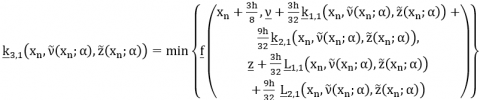
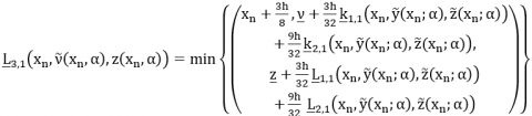
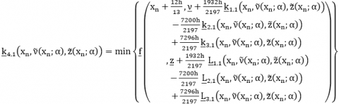
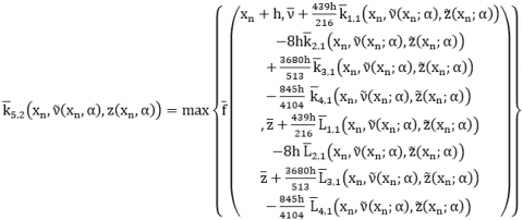
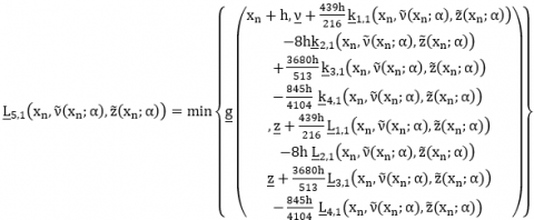
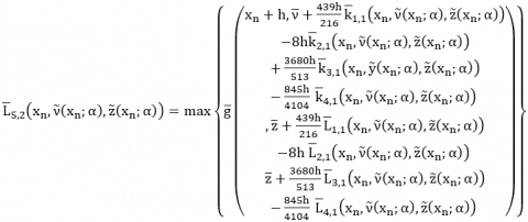
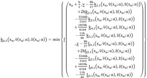
where, the $\mathrm{w}_{\mathrm{j}}$ are constants, $\underline{\mathrm{k}}_{\mathrm{j}, 1}, \overline{\mathrm{k}}_{\mathrm{j}, 2}, \underline{\mathrm{L}}_{\mathrm{j}, 1}$, and $\overline{\mathrm{L}}_{\mathrm{j}, 2}$ for $\mathrm{j}=1,2,3,4,5,6$ are defined as follows for $\tilde{v} \in\left[\underline{v}\left(\mathrm{x}_{\mathrm{n}} ; \alpha\right), \bar{v}\left(\mathrm{x}_{\mathrm{n}} ; \alpha\right)\right], \tilde{\mathrm{z}} \in$ $\left[\underline{\mathrm{z}}\left(\mathrm{x}_{\mathrm{n}} ; \alpha\right), \overline{\mathrm{z}}\left(\mathrm{x}_{\mathrm{n}} ; \alpha\right)\right]:$
$\begin{aligned} & \underline{\mathrm{k}}_{1,1}\left(\mathrm{x}_{\mathrm{n}}, \tilde{\mathrm{v}}\left(\mathrm{x}_{\mathrm{n}} ; \alpha\right), \tilde{\mathrm{z}}\left(\mathrm{x}_{\mathrm{n}} ; \alpha\right)\right)=\min \left\{\underline{\mathrm{f}}\left(\mathrm{x}_{\mathrm{n}}, \underline{v}, \underline{\mathrm{z}}\right)\right\} \\ & \overline{\mathrm{k}}_{1,2}\left(\mathrm{x}_{\mathrm{n}}, \tilde{\mathrm{y}}\left(\mathrm{x}_{\mathrm{n}} ; \alpha\right), \tilde{\mathrm{z}}\left(\mathrm{x}_{\mathrm{n}} ; \alpha\right)\right)=\max \left\{\overline{\mathrm{f}}\left(\mathrm{x}_{\mathrm{n}}, \bar{v}, \overline{\mathrm{z}}\right)\right\} \\ & \underline{\mathrm{L}}_{1,1}\left(\mathrm{x}_{\mathrm{n}}, \tilde{\mathrm{y}}\left(\mathrm{x}_{\mathrm{n}} ; \alpha\right), \tilde{\mathrm{z}}\left(\mathrm{x}_{\mathrm{n}} ; \alpha\right)\right)=\min \left\{\underline{\mathrm{g}}\left(\mathrm{x}_{\mathrm{n}}, \underline{v}, \underline{\mathrm{z}}\right)\right\} \\ & \overline{\mathrm{L}}_{1,2}\left(\mathrm{x}_{\mathrm{n}}, \tilde{\mathrm{v}}\left(\mathrm{x}_{\mathrm{n}} ; \alpha\right), \tilde{\mathrm{z}}\left(\mathrm{x}_{\mathrm{n}} ; \alpha\right)\right)=\max \left\{\overline{\mathrm{g}}\left(\mathrm{x}_{\mathrm{n}}, \bar{v}, \overline{\mathrm{z}}\right)\right\}\end{aligned}$
${{\underline{\text{k}}}_{2,1}}\left( {{\text{x}}_{\text{n}}},\widetilde{\text{v}}\left( {{\text{x}}_{\text{n}}};\alpha \right),\widetilde{\text{z}}\left( {{\text{x}}_{\text{n}}};\alpha \right) \right)=\min \left\{ \underline{\text{f}}\left( \begin{matrix} {{\text{x}}_{\text{n}}}+\frac{\text{h}}{4},\underset{\scriptscriptstyle-}{v}+\frac{\text{h}}{4}{{\underline{\text{k}}}_{1,1}}\left( {{\text{x}}_{\text{n}}},\tilde{v}\left( {{\text{x}}_{\text{n}}};\alpha \right),\widetilde{\text{z}}\left( {{\text{x}}_{\text{n}}};\alpha \right) \right) \\ \underline{\text{z}}+\frac{\text{h}}{4}{{\underline{\text{L}}}_{1,1}}\left( {{\text{x}}_{\text{n}}},\tilde{v}\left( {{\text{x}}_{\text{n}}};\alpha \right),\widetilde{\text{z}}\left( {{\text{x}}_{\text{n}}};\alpha \right) \right) \\\end{matrix} \right) \right\}$
${{\overline{\text{k}}}_{2,2}}\left( {{\text{x}}_{\text{n}}},\widetilde{\text{v}}\left( {{\text{x}}_{\text{n}}};\alpha \right),\widetilde{\text{z}}\left( {{\text{x}}_{\text{n}}};\alpha \right) \right)=\max \left\{ \overline{\text{f}}\left( \begin{matrix} {{\text{x}}_{\text{n}}}+\frac{\text{h}}{4},\bar{v}+\frac{\text{h}}{4}{{\underline{\text{k}}}_{1,2}}\left( {{\text{x}}_{\text{n}}},\tilde{v}\left( {{\text{x}}_{\text{n}}};\alpha \right),\widetilde{\text{z}}\left( {{\text{x}}_{\text{n}}};\alpha \right) \right), \\ \overline{\text{z}}+\frac{\text{h}}{4}{{\underline{\text{L}}}_{1,2}}\left( {{\text{x}}_{\text{n}}},\tilde{v}\left( {{\text{x}}_{\text{n}}};\alpha \right),\widetilde{\text{z}}\left( {{\text{x}}_{\text{n}}};\alpha \right) \right) \\\end{matrix} \right) \right\}$
${{\underline{\text{L}}}_{2,1}}\left( {{\text{x}}_{\text{n}}},\widetilde{\text{v}}\left( {{\text{x}}_{\text{n}}};\alpha \right),\widetilde{\text{z}}\left( {{\text{x}}_{\text{n}}};\alpha \right) \right)=\min \left\{ \underline{\text{g}}\left( \begin{matrix} {{\text{x}}_{\text{n}}}+\frac{\text{h}}{4},\underset{\scriptscriptstyle-}{v}+\frac{\text{h}}{4}{{\underline{\text{k}}}_{1,1}}\left( {{\text{x}}_{\text{n}}},\tilde{v}\left( {{\text{x}}_{\text{n}}};\alpha \right),\widetilde{\text{z}}\left( {{\text{x}}_{\text{n}}};\alpha \right) \right) \\ \underline{\text{z}}+\frac{\text{h}}{4}{{\underline{\text{L}}}_{1,1}}\left( {{\text{x}}_{\text{n}}},\tilde{v}\left( {{\text{x}}_{\text{n}}};\alpha \right),\widetilde{\text{z}}\left( {{\text{x}}_{\text{n}}};\alpha \right) \right) \\\end{matrix} \right) \right\}$
${{\overline{\text{K}}}_{2,2}}\left( {{\text{x}}_{\text{n}}},\widetilde{\text{v}}\left( {{\text{x}}_{\text{n}}};\alpha \right),\widetilde{\text{z}}\left( {{\text{x}}_{\text{n}}};\alpha \right) \right)=\max \left\{ \overline{\text{g}}\left( \begin{matrix} {{\text{x}}_{\text{n}}}+\frac{\text{h}}{4},\bar{v}+\frac{\text{h}}{4}{{\overline{\text{k}}}_{1,2}}\left( {{\text{x}}_{\text{n}}},\tilde{v}\left( {{\text{x}}_{\text{n}}};\alpha \right),\widetilde{\text{z}}\left( {{\text{x}}_{\text{n}}};\alpha \right) \right), \\ \overline{\text{z}}+\frac{\text{h}}{4}{{\overline{\text{L}}}_{1,2}}\left( {{\text{x}}_{\text{n}}},\tilde{v}\left( {{\text{x}}_{\text{n}}};\alpha \right),\widetilde{\text{z}}\left( {{\text{x}}_{\text{n}}};\alpha \right) \right) \\\end{matrix} \right) \right\}$
Now, the RKF5 fuzzy formula is define as follows:
$\begin{gathered}\underline{v}\left(\mathrm{x}_{\mathrm{n}+1}, \alpha\right)=\underline{v}\left(\mathrm{x}_{\mathrm{n}}, \alpha\right)+\frac{16}{135} \underline{\mathrm{k}}_{1,1}\left(\mathrm{x}_{\mathrm{n}}, \tilde{v}\left(\mathrm{x}_{\mathrm{n}} ; \alpha\right), \tilde{\mathrm{z}}\left(\mathrm{x}_{\mathrm{n}} ; \alpha\right)\right)+\frac{6656}{12825} \underline{\mathrm{k}}_{3,1}\left(\mathrm{x}_{\mathrm{n}}, \tilde{v}\left(\mathrm{x}_{\mathrm{n}} ; \alpha\right), \tilde{\mathrm{z}}\left(\mathrm{x}_{\mathrm{n}} ; \alpha\right)\right) \\ +\frac{28561}{56430} \underline{\mathrm{k}}_{4,1}\left(\mathrm{x}_{\mathrm{n}}, \tilde{v}\left(\mathrm{x}_{\mathrm{n}} ; \alpha\right), \tilde{\mathrm{z}}\left(\mathrm{x}_{\mathrm{n}} ; \alpha\right)\right)+\frac{9}{50} \underline{\mathrm{k}}_{5,1}\left(\mathrm{x}_{\mathrm{n}}, \tilde{\mathrm{v}}\left(\mathrm{x}_{\mathrm{n}} ; \alpha\right), \tilde{\mathrm{z}}\left(\mathrm{x}_{\mathrm{n}} ; \alpha\right)\right)+\frac{2}{55} \underline{\mathrm{k}}_{6,1}\left(\mathrm{x}_{\mathrm{n}}, \tilde{v}\left(\mathrm{x}_{\mathrm{n}} ; \alpha\right), \tilde{\mathrm{z}}\left(\mathrm{x}_{\mathrm{n}} ; \alpha\right)\right)\end{gathered}$
$\begin{gathered}\quad \bar{v}\left(\mathrm{x}_{\mathrm{n}+1}, \alpha\right)=\bar{v}\left(\mathrm{x}_{\mathrm{n}}, \alpha\right)+\frac{16}{135} \overline{\mathrm{k}}_{1,2}\left(\mathrm{x}_{\mathrm{n}}, \tilde{\mathrm{v}}\left(\mathrm{x}_{\mathrm{n}} ; \alpha\right), \tilde{\mathrm{z}}\left(\mathrm{x}_{\mathrm{n}} ; \alpha\right)\right)+\frac{6656}{12825} \overline{\mathrm{k}}_{3,2}\left(\mathrm{x}_{\mathrm{n}}, \tilde{\mathrm{v}}\left(\mathrm{x}_{\mathrm{n}} ; \alpha\right), \tilde{\mathrm{z}}\left(\mathrm{x}_{\mathrm{n}} ; \alpha\right)\right) \\ +\frac{28561}{56430} \overline{\mathrm{k}}_{4,2}\left(\mathrm{x}_{\mathrm{n}}, \tilde{v}\left(\mathrm{x}_{\mathrm{n}} ; \alpha\right), \tilde{\mathrm{z}}\left(\mathrm{x}_{\mathrm{n}} ; \alpha\right)\right)+\frac{9}{50} \overline{\mathrm{k}}_{5,2}\left(\mathrm{x}_{\mathrm{n}}, \tilde{v}\left(\mathrm{x}_{\mathrm{n}} ; \alpha\right), \tilde{\mathrm{z}}\left(\mathrm{x}_{\mathrm{n}} ; \alpha\right)\right)+\frac{2}{55} \overline{\mathrm{k}}_{6,2}\left(\mathrm{x}_{\mathrm{n}}, \tilde{v}\left(\mathrm{x}_{\mathrm{n}} ; \alpha\right), \tilde{\mathrm{z}}\left(\mathrm{x}_{\mathrm{n}} ; \alpha\right)\right)\end{gathered}$
$\begin{gathered}\underline{\mathrm{z}}\left(\mathrm{x}_{\mathrm{n}+1}, \alpha\right)=\underline{\mathrm{z}}\left(\mathrm{x}_{\mathrm{n}}, \alpha\right)+\frac{16}{135} \underline{\mathrm{L}}_{1,1}\left(\mathrm{x}_{\mathrm{n}}, \tilde{v}\left(\mathrm{x}_{\mathrm{n}} ; \alpha\right), \tilde{\mathrm{z}}\left(\mathrm{x}_{\mathrm{n}} ; \alpha\right)\right)+\frac{6656}{12825} \underline{\mathrm{L}}_{3,1}\left(\mathrm{x}_{\mathrm{n}}, \tilde{v}\left(\mathrm{x}_{\mathrm{n}} ; \alpha\right), \tilde{\mathrm{z}}\left(\mathrm{x}_{\mathrm{n}} ; \alpha\right)\right) \\ +\frac{28561}{56430} \underline{\mathrm{L}}_{4,1}\left(\mathrm{x}_{\mathrm{n}}, \tilde{v}\left(\mathrm{x}_{\mathrm{n}} ; \alpha\right), \tilde{\mathrm{z}}\left(\mathrm{x}_{\mathrm{n}} ; \alpha\right)\right)+\frac{9}{50} \underline{\mathrm{L}}_{5,1}\left(\mathrm{x}_{\mathrm{n}}, \tilde{v}\left(\mathrm{x}_{\mathrm{n}} ; \alpha\right), \tilde{\mathrm{z}}\left(\mathrm{x}_{\mathrm{n}} ; \alpha\right)\right)+\frac{2}{55} \underline{\mathrm{L}}_{6,1}\left(\mathrm{x}_{\mathrm{n}}, \tilde{v}\left(\mathrm{x}_{\mathrm{n}} ; \alpha\right), \tilde{\mathrm{z}}\left(\mathrm{x}_{\mathrm{n}} ; \alpha\right)\right)\end{gathered}$
$\begin{gathered}\overline{\mathrm{z}}\left(\mathrm{x}_{\mathrm{n}+1}, \alpha\right)=\underline{\mathrm{z}}\left(\mathrm{x}_{\mathrm{n}}, \alpha\right)+\frac{16}{135} \overline{\mathrm{L}}_{1,2}\left(\mathrm{x}_{\mathrm{n}}, \tilde{\mathrm{v}}\left(\mathrm{x}_{\mathrm{n}} ; \alpha\right), \tilde{\mathrm{z}}\left(\mathrm{x}_{\mathrm{n}} ; \alpha\right)\right)+\frac{6656}{12825} \overline{\mathrm{L}}_{3,2}\left(\mathrm{x}_{\mathrm{n}}, \tilde{v}\left(\mathrm{x}_{\mathrm{n}} ; \alpha\right), \tilde{\mathrm{z}}\left(\mathrm{x}_{\mathrm{n}} ; \alpha\right)\right) \\ +\frac{28561}{56430} \overline{\mathrm{L}}_{4,2}\left(\mathrm{x}_{\mathrm{n}}, \tilde{v}\left(\mathrm{x}_{\mathrm{n}} ; \alpha\right), \tilde{\mathrm{z}}\left(\mathrm{x}_{\mathrm{n}} ; \alpha\right)\right)+\frac{9}{50} \overline{\mathrm{L}}_{5,2}\left(\mathrm{x}_{\mathrm{n}}, \tilde{v}\left(\mathrm{x}_{\mathrm{n}} ; \alpha\right), \tilde{\mathrm{z}}\left(\mathrm{x}_{\mathrm{n}} ; \alpha\right)\right)+\frac{2}{55} \overline{\mathrm{L}}_{6,2}\left(\mathrm{x}_{\mathrm{n}}, \tilde{v}\left(\mathrm{x}_{\mathrm{n}} ; \alpha\right), \tilde{\mathrm{z}}\left(\mathrm{x}_{\mathrm{n}} ; \alpha\right)\right)\end{gathered}$
where, the step size $\mathrm{h}=\frac{\mathrm{b}-\mathrm{a}}{\mathrm{N}}$ and $\mathrm{N}$ is number of numerical iterations. The congruence and error analysis for fuzzy fifth order RangeKutta methods is illustrated [18] such that numerical solution $\left[\tilde{v}\left(\mathrm{x}_n\right)\right]$ convergent to the exact solution $\left[\widetilde{\mathrm{V}}\left(\mathrm{x}_n\right)\right]$ as $\mathrm{h} \rightarrow 0$ each $\alpha \in$ [0,1].
This section contains a few practise questions for the examination. To designate the absolute error for the duration of this study, we will use the notation $\widetilde{\mathrm{Er}}$, which is defined as follows:
$\widetilde{\operatorname{Er}}(\mathrm{x}, \alpha)=|\widetilde{\mathrm{V}}(\mathrm{x} ; \alpha)-\tilde{v}(\mathrm{x} ; \alpha)|=\left\{\begin{array}{l}|\underline{\mathrm{V}}(\mathrm{x} ; \alpha)-\underline{\mathrm{v}}(\mathrm{x} ; \alpha)| \\ |\overline{\mathrm{V}}(\mathrm{x} ; \alpha)-\overline{\mathrm{v}}(\mathrm{x} ; \alpha)|\end{array}\right.$
Example 5.1: Consider the following second-order linear fuzzy initial value problem [22]:
$\left\{\begin{array}{c}\tilde{v}^{\prime \prime}-4 \tilde{v}^{\prime}+4 \tilde{v}=4 \mathrm{x}-4, \mathrm{x} \geq 0 \\ \tilde{v}(0)=(2+\alpha, 4-\alpha), \tilde{v}^{\prime}(0)=(3+2 \alpha, 9-2 \alpha)\end{array}\right.$ (7)
The exact analytical solution of Eq. (7) is presented as follow (See study [22]):
$\left\{\begin{array}{l}\underline{\mathrm{V}}(\mathrm{x} ; \alpha)=(2+\alpha) \mathrm{e}^{2 \mathrm{x}}+(-1+\alpha) \mathrm{xe}^{2 \mathrm{x}}+\mathrm{x} \\ \overline{\mathrm{V}}(\mathrm{x} ; \alpha)=(4-\alpha) \mathrm{e}^{2 \mathrm{x}}+(1-\alpha) \mathrm{xe}^{2 \mathrm{x}}+\mathrm{x}\end{array}\right.$
According to Section 4, Eq. (7) can be written into first order linear system of FIVPs as follows:
$\left\{\begin{array}{l}\tilde{v}^{\prime}(\mathrm{x} ; \mathrm{r})=\tilde{\mathrm{z}}(\mathrm{x} ; \alpha) \\ \tilde{v}(0 ; \alpha)=[2+\alpha, 4-\alpha] \\ \tilde{\mathrm{z}}^{\prime}(\mathrm{x} ; \alpha)=4-4 \mathrm{x}+4 \tilde{\mathrm{z}}(\mathrm{t} ; \mathrm{r})-4 \tilde{v}(\mathrm{x} ; \alpha) \\ \tilde{\mathrm{z}}(0 ; \alpha)=[3+2 \alpha, 9-2 \alpha]\end{array}\right.$ (8)
where,
$\left\{\begin{array}{c}\tilde{\mathrm{f}}(\mathrm{x}, \tilde{\mathrm{v}}, \tilde{\mathrm{z}} ; \alpha)=\tilde{\mathrm{z}}(\mathrm{x} ; \alpha) \\ \tilde{\mathrm{g}}(\mathrm{x}, \tilde{\mathrm{v}}, \tilde{\mathrm{z}} ; \alpha)=4-4 \mathrm{x}+4 \tilde{\mathrm{z}}(\mathrm{t} ; \mathrm{r})-4 \tilde{v}(\mathrm{x} ; \alpha)\end{array}\right.$ (9)
Applying Eqs. (4)-(5) in fuzzy RKF5 in Section 4 to obtain the numerical solution of Eq. (7). Next, the numerical comparison is displayed in Tables 1-2 between fuzzy RKF5 at N=10 and the UFCM [20] for x=0.001 at different values of $\alpha \in[0,1]$ and summarized in Figure 1 as below:
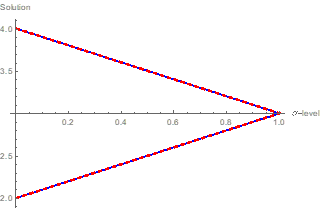
Figure 1. Exact and RKF5 solutions of Eq. (7) at x=0.001 for N=10 and for all $\alpha \in[0,1]$
Clearly that the numerical results of Eq. (2) in Tables 1-2 show that RKF5 performance over UFCM [22] at same values of x=0.001 and $\alpha \in[0,1]$. Moreover, Tables 1-2 and Figure 1 show that RKM5 solution compared with exact solution of Eq. (7) satisfies the fuzzy number properties in Section 2 in the form of a triangular fuzzy number. The next step is to show how the RKF5 perform with different number of iterations at x=1 and different values of $\alpha \in[0,1]$ as displayed in Tables 3-4 and Figures 2-3.
Table 1. Comparison between the accuracy of RKF5 at N=10 and UFCM at x=0.001 of the lower solution for Eq. (7)
|
α |
$\underline{\mathbf{V}}(\mathbf{x} ; \boldsymbol{\alpha})$ |
RKF5 $\underline{\mathbf{v}}(\mathbf{x} ; \boldsymbol{\alpha})$ |
$\underline{\mathbf{E}}r (\mathbf{x} ; \boldsymbol{\alpha})$ |
UFCM [20] |
|
0 |
2.0029999986653326 |
2.002999998665332 |
4.4408920985×10⁻¹⁶ |
0.00099871222831 |
|
0.2 |
2.2034003989321325 |
2.2034003989321325 |
0 |
0.00119975860278 |
|
0.4 |
2.4038007991989327 |
2.4038007991989323 |
4.4408920985×10⁻¹⁶ |
0.00140080497724 |
|
0.6 |
2.604201199465733 |
2.604201199465733 |
0 |
0.00160185135171 |
|
0.8 |
2.804601599732533 |
2.8046015997325324 |
4.4408920985×10⁻¹⁶ |
0.00180289772617 |
|
1.0 |
3.0050019999993327 |
3.0050019999993327 |
0 |
0.00200394410063 |
Table 2. Comparison between the accuracy of RKF5 at N=10 and UFCM at x=0.001 of the upper solution for Eq. (7)
|
α |
$\overline{\mathrm{V}}(\mathrm{x} ; \alpha)$ |
$\operatorname{RKF5} \bar{v}(x ; \alpha)$ |
$\overline{\mathrm{E}} \mathrm{r}(\mathrm{x} ; \alpha)$ |
UFCM [20] |
|
0 |
4.0090080053360015 |
4.0090080053360015 |
0 |
0.00101009737569 |
|
0.2 |
3.808607605069201 |
3.8086076050692004 |
4.440892098500626×10⁻¹⁶ |
0.00080905100122 |
|
0.4 |
3.608207204802401 |
3.608207204802401 |
0 |
0.00060800462676 |
|
0.6 |
3.407806804535601 |
3.4078068045356003 |
8.881784197001252×10⁻¹⁶ |
0.00040695825230 |
|
0.8 |
3.207406404268801 |
3.207406404268801 |
0 |
0.00020591187783 |
|
1.0 |
3.0070060040020006 |
3.007006004002 |
4.440892098500626×10⁻¹⁶ |
0.00000486550337 |
Table 3. Results analysis of RKF5 for N=10 at x=1 of the lower solution for Eq. (7)
|
α |
$\underline{V}(\mathrm{x} ; \alpha)$ |
RKF5 $\underline{\mathbf{v}}(\mathbf{x} ; \boldsymbol{\alpha})$ |
$\underline{\operatorname{Er}}(\mathrm{x} ; \alpha)$ |
|
0 |
1 |
1.000021468482932 |
0.00002146848293205217 |
|
0.2 |
2.4778112197861297 |
2.4778319535483457 |
0.000020733762216007534 |
|
0.4 |
3.9556224395722595 |
3.9556424386137623 |
0.00001999904150284948 |
|
0.6 |
5.433433659358389 |
5.433452923679174 |
0.000019264320784806443 |
|
0.8 |
6.911244879144521 |
6.911263408744585 |
0.000018529600064098872 |
|
1.0 |
8.38905609893065 |
8.389073893809996 |
0.000017794879346055836 |
|
α |
$\overline{\mathrm{V}}(\mathrm{x} ; \alpha)$ |
RKF5 $\bar{v}(\mathrm{x} ; \alpha)$ |
$\overline{\operatorname{Er}}(\mathrm{x} ; \alpha)$ |
|
0 |
30.5562243957226 |
30.556209701308262 |
0.000014694414339544437 |
|
0.2 |
29.078413175936472 |
29.078399216242854 |
0.000013959693617948687 |
|
0.4 |
27.600601956150342 |
27.60058873117743 |
0.000013224972910563793 |
|
0.6 |
26.122790736364212 |
26.122778246112027 |
0.00001249025218541533 |
|
0.8 |
24.644979516578083 |
24.644967761046622 |
0.000011755531460266866 |
|
1.0 |
23.16716829679195 |
23.167168296665125 |
1.268247729058202×10⁻¹⁰ |
Table 4. Results analysis of RKF5 for N=100 at x=1 of the lower solution for Eq. (7)
|
α |
$\underline{V}(\mathrm{x} ; \alpha)$ |
RKF5 $\underline{\mathbf{v}}(\mathbf{x} ; \boldsymbol{\alpha})$ |
$\underline{\operatorname{Er}}(\mathrm{x} ; \alpha)$ |
|
0 |
1 |
1.0000000002530203 |
2.53020271401283 ×10⁻¹⁰ |
|
0.2 |
2.4778112197861297 |
2.4778112200306923 |
2.445625923996886×10⁻¹⁰ |
|
0.4 |
3.9556224395722595 |
3.9556224398083595 |
2.361000284167858×10⁻¹⁰ |
|
0.6 |
5.433433659358389 |
5.433433659586035 |
2.276454580396603×10⁻¹⁰ |
|
0.8 |
6.911244879144521 |
6.911244879363703 |
2.191820058783378×10⁻¹⁰ |
|
1.0 |
8.38905609893065 |
8.389056099141396 |
2.107451990696060×10⁻¹⁰ |
|
α |
$\overline{\mathrm{V}}(\mathrm{x} ; \alpha)$ |
RKF5 $\bar{v}(\mathrm{x} ; \alpha)$ |
$\overline{\operatorname{Er}}(\mathrm{x} ; \alpha)$ |
|
0 |
30.5562243957226 |
30.556224395553485 |
1.691162765382614×10⁻¹⁰ |
|
0.2 |
29.078413175936472 |
29.07841317577579 |
1.60682134264789×10⁻¹⁰ |
|
0.4 |
27.600601956150342 |
27.600601955998115 |
1.522266757092438×10⁻¹⁰ |
|
0.6 |
26.122790736364212 |
26.122790736220484 |
1.43728584589553×10⁻¹⁰ |
|
0.8 |
24.644979516578083 |
24.644979516442778 |
1.35305100457117×10⁻¹⁰ |
|
1.0 |
23.16716829679195 |
23.167168296665125 |
1.268247729058202×10⁻¹⁰ |
(a)
(b)
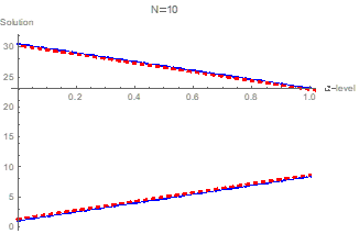
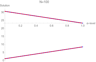
Figure 2. Exact and RKF5 solutions of Eq. (7) at x=1 for N=100 and for all $\alpha \in[0,1]$
From Tables 1-2, the increasing number of RKF5 iterations perform better accuracy and convergent to the exact solution as mentioned in the convergence theory of Range Kutta methods for each level $\alpha \in[0,1]$. Besides, Tables 3-4 and Figures 2-3 show that RKF5 solution compared with exact solution of Eq. (7) satisfies the fuzzy number properties in the form of a trapezoidal fuzzy number.
Example 5.2: Consider the following second-order linear fuzzy initial value problem [17]:
$\left\{\begin{array}{l}\tilde{v}^{\prime \prime}+\tilde{v}=x, x \geq 0 \\ \tilde{v}(0)=(0.9+0.1 \alpha, 1.1-0.1 \alpha) \\ \tilde{v}^{\prime}(0)=(1.8+0.2 \alpha, 2.2-0.2 \alpha)\end{array}\right.$ (10)
It can be checked that exact analytical solution of Eq. (10) is given in study [17] as follows:
$\left\{\begin{array}{l}\underline{\mathrm{V}}(\mathrm{x} ; \alpha)=\left(\frac{4}{5}+\frac{1}{5} \alpha\right) \sin \mathrm{x}+\left(\frac{9}{10}+\frac{1}{10} \alpha\right) \cos \mathrm{x} \\ \overline{\mathrm{V}}(\mathrm{x} ; \alpha)=\left(\frac{6}{5}-\frac{1}{5} \alpha\right) \sin \mathrm{x}+\left(\frac{11}{10}-\frac{1}{10} \alpha\right) \cos \mathrm{x}\end{array}\right.$
According to Section 4, Eq. (7) can be written into first-order linear system of FIVPs as follows:
$\left\{\begin{array}{l}\tilde{v}^{\prime}(\mathrm{x} ; \mathrm{r})=\tilde{\mathrm{z}}(\mathrm{x} ; \alpha), \\ \tilde{v}(0 ; \alpha)=[0.9+0.1 \alpha, 1.1-0.1 \alpha], \\ \tilde{\mathrm{z}}^{\prime(\mathrm{x} ; \alpha)}=\mathrm{x}-\tilde{v}(\mathrm{x} ; \alpha), \\ \tilde{\mathrm{z}}(0 ; \alpha)=[1.8+0.2 \alpha, 2.2-0.2 \alpha],\end{array}\right.$ (11)
where,
$\left\{\begin{array}{l}\tilde{f}(x, \tilde{v}, \tilde{z} ; \alpha)=\tilde{z}(x ; \alpha), \\ \tilde{g}(x, \tilde{v}, \tilde{z} ; \alpha)=x-\tilde{v}(x ; \alpha) .\end{array}\right.$ (12)
Applying Eqs. (10)-(12) in fuzzy RKF5 in Section 4 to obtain the numerical solution of Eq. (10). Next, the numerical comparison is displayed in Tables 5-6 between fuzzy RKF5 and fifth-order Fuzzy Improved Runge-Kutta Nystrom method with four stages (FIRKN5 [17]) for N=10, x=1 and different values of $\alpha \in[0,1]$ and summarized in Figure 4 as below:
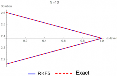
Figure 3. Exact and RKF5 solutions of Eq. (6) at x=1 for N=10 and for all $\alpha \in[0,1]$
Figure 4. Exact and RKF5 solutions of Eq. (13) at x=0.1 for N=10 and for all $\alpha \in[0,1]$
Noted from Tables 5-6 that the numerical results of Eq. (10) show that RKF5 is performed better than FIRKN5 [17] at same values of x=1, N=10 and $\alpha \in[0,1]$. Also, Tables 3-4 and Figure 3 show that RKF5 solution compare with exact solution of Eq. (10) satisfies the fuzzy number properties in in the form of triangular fuzzy number.
Table 5. Comparison between the accuracy of RKF5 and FIRKN5 at x=1 and N=10 of the lower solution for Eq. (10)
|
α |
$\underline{V}(x ; \alpha)$ |
RKF5 $\underline{v}(\mathrm{x} ; \alpha)$ |
$\underline{\operatorname{Er}}(\mathrm{x} ; \alpha)$ |
FIRKN5 |
|
0 |
2.1594488631276434 |
2.159448873854798 |
1.072715472005825×10⁻⁹ |
3.13×10⁻⁸ |
|
0.2 |
2.203913748637322 |
2.2039137597636347 |
1.112631276001252×10⁻⁹ |
3.25×10⁻⁸ |
|
0.4 |
2.2483786341470005 |
2.2483786456724704 |
1.152546991178837×10⁻⁹ |
3.37×10⁻⁸ |
|
0.6 |
2.292843519656679 |
2.2928435315813065 |
1.192462750765344×10⁻⁹ |
3.49×10⁻⁸ |
|
0.8 |
2.337308405166358 |
2.3373084174901417 |
1.232378377125087×10⁻⁸ |
3.61×10⁻⁸ |
|
1.0 |
2.3817732906760365 |
2.381773303398978 |
1.272294136711593×10⁻⁸ |
3.37×10⁻⁸ |
Table 6. Comparison between the accuracy of RKF5 and FIRKN5 at x=1 and N=10 of the upper solution for Eq. (10)
|
α |
$\overline{\mathrm{V}}(\mathrm{x} ; \alpha)$ |
$\operatorname{RKF} 5 \bar{v}(\mathrm{x} ; \alpha)$ |
$\overline{\operatorname{Er}}(\mathrm{x} ; \alpha)$ |
FIRKN5 |
|
0 |
2.6040977182244296 |
2.604097732943158 |
1.471872845826283×10⁻⁹ |
4.23×10⁻⁸ |
|
0.2 |
2.559632832714751 |
2.559632847034322 |
1.431957086239776×10⁻⁹ |
4.20×10⁻⁸ |
|
0.4 |
2.5151679472050725 |
2.515167961125486 |
1.39204132665327×10⁻⁹ |
4.09×10⁻⁸ |
|
0.6 |
2.470703061695394 |
2.47070307521665 |
1.352125611475685×10⁻⁸ |
3.97×10⁻⁸ |
|
0.8 |
2.426238176185715 |
2.426238189307814 |
1.3122098962981×10⁻⁸ |
3.85×10⁻⁸ |
|
1.0 |
2.3817732906760365 |
2.381773303398978 |
1.272294136711593×10⁻⁸ |
3.73×10⁻⁸ |
Example 5.3: Consider the following second-order non-linear fuzzy initial value problem [19]:
$\left\{\begin{array}{l}\tilde{v}^{\prime \prime}+\left(\tilde{v}^{\prime}\right)^2=0, \mathrm{x} \geq 0 \\ \tilde{v}(0)=(\alpha, 2-\alpha), \tilde{v}^{\prime}(0)=(1+\alpha, 3-\alpha)\end{array}\right.$ (13)
The exact analytical solution of Eq. (13) is equivalent to the exact solution in study [19] as follows:
$\left\{\begin{array}{l}\underline{\mathrm{V}}(\mathrm{x} ; \alpha)=r-\log \left[-\frac{1}{-1-r}\right]+\log \left[-\frac{1}{-1-r}+\mathrm{x}\right] \\ \overline{\mathrm{V}}(\mathrm{x} ; \alpha)=2-r-\log \left[-\frac{1}{-3+r}\right]+\log \left[-\frac{1}{-3+r}+\mathrm{x}\right]\end{array}\right.$
According to Section 4, Eq. (9) can be written into first order non-linear system of FIVPs as follows:
$\left\{\begin{array}{l}\tilde{v}^{\prime}(\mathrm{x} ; \mathrm{r})=\tilde{\mathrm{z}}(\mathrm{x} ; \alpha), \\ \tilde{v}(0 ; \alpha)=[\alpha, 1+\alpha], \\ \tilde{v}^{\prime}(\mathrm{x} ; \alpha)=[\tilde{\mathrm{z}}(\mathrm{x} ; \alpha)]^2, \\ \tilde{v}(0 ; \alpha)=[2-\alpha, 3-\alpha],\end{array}\right.$ (14)
where,
$\left\{\begin{array}{l}\tilde{\mathrm{f}}(\mathrm{x}, \tilde{\mathrm{v}}, \tilde{\mathrm{z}} ; \alpha)=\tilde{\mathrm{z}}(\mathrm{x} ; \alpha) \\ \tilde{\mathrm{g}}(\mathrm{x}, \tilde{\mathrm{v}}, \tilde{\mathrm{z}} ; \alpha)=[\tilde{\mathrm{z}}(\mathrm{x} ; \alpha)]^2\end{array}\right.$ (15)
Applying Eqs. (13)-(15) in fuzzy RKF5 in Section 4 to obtain the numerical solution of Eq. (13). Additionally, the numerical comparison is displayed in Tables 7-8 between fuzzy RKF5 and standard fifth-order Fuzzy Runge-Kutta method (RK56 [19]) for N=10, x=0.1 and different values of $\alpha \in[0,1]$and summarized in Figure 4.
One can noted from Tables 7-8 that the numerical results of Eq. (13) show that RKF5 is performed better than RK56 [19] at the same values of x=0.1, N=10 and $\alpha \in[0,1]$. Also, Tables 7-8 and Figure 4 show that RKF5 solution compared with exact solution of Eq. (13) satisfies the fuzzy number properties in the form of a triangular fuzzy number.
Table 7. Comparison between the accuracy of RKF5 and RK56 at x=0.1 and N=10 of the lower solution for Eq. (13)
|
α |
$\underline{\mathrm{V}}(\mathrm{x} ; \alpha)$ |
RKF5 $\underline{v}(\mathrm{x} ; \alpha)$ |
$\underline{\operatorname{Er}}(\mathrm{x} ; \alpha)$ |
RK56 |
|
0 |
0.09531017980432493 |
0.09531017980434438 |
1.94427807187480×10⁻¹⁴ |
9.8449026708635×10⁻¹⁴ |
|
0.25 |
0.36778303565638343 |
0.367783035656456 |
7.255307465925398×10⁻¹⁴ |
3.4927616354707×10⁻¹³ |
|
0.50 |
0.6397619423751586 |
0.6397619423753707 |
2.120525977034049×10⁻¹³ |
9.7144514654701×10⁻¹³ |
|
0.75 |
0.9112681475961222 |
0.9112681475966461 |
5.239142453206114×10⁻¹³ |
2.2859492077031×10⁻¹² |
|
1.00 |
1.1823215567939545 |
1.1823215567951029 |
1.148414696672262×10⁻¹² |
4.7628567756419×10⁻¹² |
Table 8. Comparison between the accuracy of RKF5 and RK56 at x=0.1 and N=10 of the upper solution for Eq. (13)
|
α |
$\overline{\mathrm{V}}(\mathrm{x} ; \alpha)$ |
$\operatorname{RKF5} \bar{v}(\mathrm{x} ; \alpha)$ |
$\overline{\operatorname{Er}}(\mathrm{x} ; \alpha)$ |
RK56 |
|
0 |
2.2623642644674913 |
2.262364264479998 |
1.250688441700731×10⁻¹¹ |
4.22675228151092×10⁻¹¹ |
|
0.25 |
1.9929461786103895 |
1.992946178617871 |
7.481570918344005×10⁻¹² |
2.66238142643260×10⁻¹¹ |
|
0.50 |
1.7231435513142097 |
1.7231435513184756 |
4.265920949819701×10⁻¹² |
1.59825486178988×10⁻¹¹ |
|
0.75 |
1.4529408439966902 |
1.4529408439989848 |
2.294608947295273×10⁻¹² |
9.04853969529995×10⁻¹² |
|
1.00 |
1.1823215567939545 |
1.1823215567951029 |
1.148414696672262×10⁻¹² |
4.76285677564192×10⁻¹² |
This research proposes a computational approach for solving fuzzy differential equations (FDEs). The approach is based on using the RKF5 method to solve linear and nonlinear second-order FIVPs with fuzzy initial conditions. To make the RKF5 method suitable for solving these problems, a complete fuzzy analysis is presented, which evaluates the method's performance under fuzzy properties using principles of fuzzy set theory. The proposed method is tested on several examples with different numbers of iterations and input domains, using various levels of fuzzy sets. The results show that the RKF5 method performs better than other existing methods in terms of accuracy. The findings are presented in tables that follow the characteristics of fuzzy numbers, which validate the RKF5 fuzzy numerical solution. Overall, this research presents a promising approach for solving fuzzy FDEs using the RKF5 method and provides insights into the behaviour of fuzzy systems under different input conditions.
The authors would like to thank Mustansiriyah University (WWW.uomustansiriyah.edu.iq) Baghdad – Iraq for its support in the present work.
|
FIVPs |
Fuzzy Initial Value Problems |
|
FDEs |
Fuzzy Differential Equations |
|
RKF5 |
Fifth order Range-Kutta Fehlberg Method |
|
UFCM |
Undetermined Fuzzy Coefficients Method |
|
TN |
Truncation Error |
|
Greek symbols |
|
|
$\alpha$ |
Fuzzy Level Sets |
|
$\delta_{\mathrm{N}}$ |
Value Bouand of Transection Error |
|
$\gamma_{j n}$ |
Range- Kutta Matrix Elements |
|
$\tau$ |
Element of Fuzzy Membership Function |
|
Subscripts |
|
|
n |
Point Index in the Intirval |
|
j |
Index of Ranhe-Kutta Stages |
[1] Nemati, K., Matinfar, M. (2008). An implicit method for fuzzy parabolic partial differential equations. Journal of Nonlinear Sciences and Applications, 1(2): 61-71. https://doi.org/10.22436/jnsa.001.02.02
[2] Kaleva, O. (1987). Fuzzy differential equation. Fuzzy Sets Systems, 24(3): 301-317. https://doi.org/10.1016/0165-0114(87)90029-7
[3] Hossain, M.J., Alam, M.S., Hossain, M.B. (2017). A study on numerical solutions of second order initial value problems (IVP) for ordinary differential equations with fourth order and Butcher’s fifth order Runge-Kutta methods. American Journal of Computational and Applied Mathematics, 7(5): 129-137. https://doi.org/10.5923/j.ajcam.20170705.02
[4] Tareque, H., Musa, M., Babul. H. (2017). A numerical study to predict the evolution of yellow fever diseases using fourth order Runge-Kutta method. International Journal of Scientific and Engineering Research, 8(10): 1-21. https://doi.org/10.14299/ijser.2017.10.004
[5] Rahman, A., Reza, M. (2014). A new compact finite difference method for solving the generalized long wave equation. Numerical Functional Analysis and Optimization, 35(2): 133-152. https://doi.org/10.1080/01630563.2013.830128
[6] Maryam, A., Hamzeh, Z., Ahmad, I., Ali, F.J. (2021). Fuzzy numerical solution via finite difference scheme of wave equation in double parametrical fuzzy number form. Mathematics, 9(6): 1-15. https://doi.org/10.3390/math9060667
[7] Ali, F.J., Azizan, S., Hamzeh, H.Z. (2018). Numerical solution of second-order fuzzy nonlinear two-point boundary value problems using combination of finite difference and Newton’s methods. Neural Computing and Applications, 30(10): 3167-3175. https://doi.org/10.1007/s00521-017-2893-z
[8] Omer, A., Omer, O. (2013). A Pray and predator model with fuzzy initial values. Hacettepe Journal of Mathematic sand Statistics, 41(3): 387-395. https://dergipark.org.tr/en/download/article-file/86413.
[9] Tapaswini, S., Chakraverty, S. (2013). Numerical solution of fuzzy arbitrary order predator-prey equations. Applications and Applied Mathematics: An International Journal (AAM), 8(2): 20. https://digitalcommons.pvamu.edu/aam/vol8/iss2/20.
[10] El Naschie, M.S. (2005). From experimental quantum optics to quantum gravity via a fuzzy Kähler manifold. Chaos, Solitons & Fractals, 25(5): 969-977. https://doi.org/10.1016/j.chaos.2005.02.028
[11] Abbod, M.F., von Keyserlingk, D.G., Linkens, D.A., Mahfouf, M. (2001). Survey of utilisation of fuzzy technology in medicine and healthcare. Fuzzy Sets and Systems, 120(2): 331-349. https://doi.org/10.1016/S0165-0114(99)00148-7
[12] Kudryashov, N.A. (2020). Method for finding highly dispersive optical solitons of nonlinear differential equations. Optik, 206: 163550. https://doi.org/10.1016/j.ijleo.2019.163550
[13] Bulut, H., Baskonus, H.M., Belgacem, F.B.M. (2013). The analytical solution of some fractional ordinary differential equations by the Sumudu transform method. In Abstract and Applied Analysis. https://doi.org/10.1155/2013/203875
[14] Julyan, H.E., Oreste, P. (1992). The dynamics of Runge-Kutta methods. International Journal of Bifurcation and Chaos, 2(3): 27-449. https://doi.org/10.1142/S0218127492000641
[15] Parandin, N. (2012). Numerical solution of fuzzy differential equations of n th-order by Runge–Kutta method. Neural Computing and Applications, 21: 347-355. https://doi.org/10.1007/s00521-012-0928-z
[16] Ji, X, Zhou, J. (2017). Solving high-order uncertain differential equations via Runge-Kutta method. IEEE Transactions on Fuzzy Systems, 26(3): 1379-1386. https://doi.org/10.1109/TFUZZ.2017.2723350
[17] Rabiei, F., Ismail, F., Ahmadian, A., Salahshour, S. (2013). Numerical solution of second-order fuzzy differential equation using improved Runge-Kutta Nystrom method. Mathematical Problems in Engineering, 2013: 1-10. https://doi.org/10.1155/2013/803462
[18] Jameela, A., Anakira, N.R., Alomari, A.K., Hashim, I., Shakhatreh, M.A. (2016). Numerical solution of n’th order fuzzy initial value problems by six stages. Journal of Nonlinear Science Applications, 9(2): 627-640. https://doi.org/10.22436/jnsa.009.02.26
[19] Jameel, A.F., Anakira, N.R., Shather, A.H., Azizan, S., Alomari, A.K. (2020). Numerical algorithm for solving second order nonlinear fuzzy initial value problems. International Journal of Electrical and Computer Engineering, 10(6): 6497-6506. https://doi.org/10.11591/ijece. v10i6.pp6497-6506
[20] Guo, X., Shang, D. (2013). Approximate solution of th-order fuzzy linear differential equations. Mathematical Problems in Engineering. https://doi.org/10.1155/2013/406240
[21] Bodjanova, S. (2006). Median alpha-levels of a fuzzy number. Fuzzy Sets and Systems, 157(7): 879-891. https://doi.org/10.1016/j.fss.2005.10.015
[22] Dubois, D., Prade, H. (1982). Towards fuzzy differential calculus part 3: Differentiation. Fuzzy Sets and Systems, 8(3): 225-233. https://doi.org/10.1016/S0165-0114(82)80001-8
[23] Zhang, X., Ma, W., Chen, L. (2014). New similarity of triangular fuzzy number and its application. The Scientific World Journal. https://doi.org/10.1155/2014/215047
[24] Zadeh, L.A. (2005). Toward a generalized theory of uncertainty (GTU)––An outline. Information Sciences, 172(1-2): 1-40. https://doi.org/10.1155/2014/215047
[25] Goetschel Jr, R., Voxman, W. (1986). Elementary fuzzy calculus. Fuzzy Sets and Systems, 18(1): 31-43. https://doi.org/10.1016/0165-0114(86)90026-6
[26] Jain, R.K., Jain, M.K. (1972). Optimum Runge-Kutta-Fehlberg methods for second-order differential equations. IMA Journal of Applied Mathematics, 10(2): 202-210. https://doi.org/10.1093/imamat/10.2.202
[27] Simos, T.E. (1993). A Runge-Kutta Fehlberg method with phase-lag of order infinity for initial-value problems with oscillating solution. Computers & Mathematics with Applications, 25(6): 95-101. https://doi.org/10.1016/0898-1221(93)90303-D
[28] Polla, G. (2013). Comparing accuracy of differential equation results between Runge-Kutta fehlberg methods, and adams-moulton methods. Applied Mathematical Sciences, 7(103): 5115-5127. https://doi.org/10.12988/ams.2013.36314
[29] Fae’q, A., Radwan, A. (2002). Solution of initial value problem using fifth order Runge–Kutta Method Using Excel Spreadsheet. Pakistan Journal of Applied Sciences, 2(1): 44-47. https://doi.org/10.3923/jas.2002.44.47
[30] Lindfield, G., Penny, J. (2018). Numerical Methods: Using MATLAB. Academic Press, USA.