Iman Ameer Ahmad*![]() | Muna Mohammed Jawad Al-Nayar
| Muna Mohammed Jawad Al-Nayar![]() | Ali M. Mahmood
| Ali M. Mahmood![]()
© 2023 IIETA. This article is published by IIETA and is licensed under the CC BY 4.0 license (http://creativecommons.org/licenses/by/4.0/).
OPEN ACCESS
Wireless Sensor Networks (WSNs) have emerged as a pivotal technology interlinked with numerous burgeoning sectors. Myriad sensor nodes, diverse in nature, constitute these networks, which are dispersed within a given environment to collect and relay pertinent data to a central station. Given the typical deployment of sensor nodes—bearing limited energy reserves and often stationed at extensive distances for prolonged periods—energy conservation becomes a paramount concern for enhancing the network's lifespan. One avenue explored to address this challenge involves the clustering of sensor nodes within the network. This study introduces a dynamic approach for clustering nodes in WSNs, designed to accommodate mobile nodes. The approach leverages an enhanced version of the k-means algorithm in tandem with a novel cluster head selection method, capable of clustering even moving nodes. This strategy proposes an innovative solution to select cluster heads, aiming to reduce the energy consumption of nodes and augment reliability during data transmission within sensor networks.
clustering algorithm, energy efficiency, K-means algorithm, mobile wireless sensor network
The burgeoning technology of the Internet of Things (IoT) facilitates the ubiquitous exchange of data across a multitude of communication networks. In essence, IoT empowers devices to perform operations such as measurement, judgment, and information sharing. The careful selection of appropriate technologies and protocols for communication between diverse objects is paramount, given the profound impact this technology is expected to have on numerous facets of human existence [1-3].
One such technology is the wireless sensor network (WSN), which comprises numerous tiny sensor nodes with constrained communication and computational capabilities. These nodes are tasked with collecting and transmitting data from their environments to users or base stations [4-6].
At present, advancements in wireless communication technology coupled with the miniaturization of integrated circuits have laid the foundation for the evolution of WSNs [4, 7, 8]. The potential applicability of these networks in a variety of industries – including network intrusion detection, environmental monitoring, healthcare, security, and natural disaster warning systems – has attracted significant interest among researchers. One of the key advantages of WSNs is their ability to operate in harsh, unsupervised conditions where traditional human monitoring methods may be risky, ineffective, or even impractical. Consequently, sensors are expected to be dispersed randomly, and largely unsupervised, across the target area, leading to the formation of a transient network [9, 10].
A fundamental challenge associated with WSNs, especially those covering large areas, is the finite and irreplaceable power resources of the sensor nodes, which are typically powered by small batteries. In many applications, replacing sensor nodes once their energy levels dwindle can prove challenging. Therefore, it is critical to minimize the power consumption of each node and extend the lifespan of the network, particularly since sensor nodes may be deployed in hazardous and inaccessible locations without access to electricity or recharging facilities.
One strategy proposed to address these challenges in wireless sensor networks (WSNs) is clustering. Clustering involves segmenting nodes into distinct groups or clusters, each with a selected cluster head. The cluster head of each group is responsible for receiving sensor data, aggregating it, and subsequently transmitting it to the base station, either independently or with assistance from nearby cluster heads. Clustering in WSNs is a practical method for reducing the network's energy consumption and extending its lifespan. However, achieving load balancing among cluster heads is a challenging but essential task for the sustained operation of WSNs. This is because cluster heads bear an additional burden for tasks such as data collection, aggregation, transmission to the base station, route selection for data transmission, and network stabilization based on the remaining energy, all of which are crucial for maximizing node uptime [11].
While various clustering techniques have been proposed for WSNs, the primary objective of this study is to create stable clusters in environments with moving nodes [12]. The proposed clustering approaches are influenced by various factors, including the nodes' deployment and configuration strategies, the network architecture utilized, cluster head (CH) node characteristics, and the network's operational model. Sensors within clusters may elect a CH, or the network designer may predefine one. Alternatively, a CH can be a sensor or node with superior resources.
Clustering offers several additional benefits, such as facilitating network scalability and localizing the route set of each cluster, thereby reducing the size of the routing table stored at each node [13]. By restricting inter-cluster communications to CHs and preventing duplicate information transmission between sensor nodes, clustering can also conserve communication bandwidth [14]. Further, clustering can decrease the cost of topology maintenance by stabilizing the network topology at the sensor level. Clustering also allows the cluster head to adopt optimal management procedures to improve network performance, prolong the network's lifetime, and extend the battery life of individual sensors [12]. For instance, the cluster head may schedule the cluster's activity to allow nodes to frequently enter a low-power sleep mode, thus conserving energy. Additionally, a cluster head could aggregate data collected by sensors within its cluster, reducing the volume of transmitted packets [15].
With the rapid advancements in wireless and location technology, there is an influx of location data from mobile clients, vehicles (cars, buses, planes), and even animals. This proliferation of data necessitates effective location information management and analytical methodologies. Node mobility in a WSN can be harnessed to enhance data collection and analysis. For example, mobile nodes could be used to connect disconnected parts of the network. Moreover, node mobility can help improve a WSN's energy usage and longevity. For instance, mobile sinks can be moved towards data sources or sensor nodes to prevent communication bottlenecks. However, topological changes induced by the use of mobile nodes must be addressed before data collection can resume [16].
This paper proposes a strategy for clustering moving objects, utilizing the well-established k-means clustering algorithm and a novel cluster head selection method. The paper is structured as follows: Section 2 discusses related works, Section 3 details the proposed method, Section 4 evaluates the proposed method, and Section 5 provides the conclusion.
In summary, optimizing the energy consumption of sensors in wireless sensor networks (WSNs) using the clustering method is a highly effective strategy for reducing sensor power consumption, extending node lifespan, and ultimately prolonging the network's operational duration.
Numerous methods have been proposed for the static clustering of sensor nodes. These static approaches segment sensor nodes based on parameters such as location, residual energy, link quality, or processing capacity. In these static methods, sensor nodes are assumed to be stationary and without mobility. However, in many applications of WSNs, nodes are mobile and can change their position.
In applications proposed for these networks, including industrial, military, target tracking, and environmental monitoring contexts, some or all nodes may be mobile. When static approaches are used to cluster nodes in these applications, the clustering process must be redone in each round. This is because the members of the cluster, or even the cluster head, may change location, leading to the collapse of the cluster structure. This scenario drains the network energy since changing the cluster structure and reapplying the clustering process necessitates the transmission of many messages within the network so nodes can identify the cluster head and cluster members. This process is particularly challenging for sensor networks that are highly sensitive to energy loss.
Node mobility induces frequent changes in the network architecture in Mobile Wireless Sensor Networks (MWSNs), which can separate sensor nodes from their cluster heads. This leads to considerable data loss and reduced data rates. As a result, clustering methods like LEACH-Mobile, LEACH-ME, etc., were developed [17-20]. These methods consider node mobility alongside node energy and location. However, since these methods rely on a two-layer distribution, they may not achieve optimal scalability and energy efficiency, even though they manage node mobility and enhance data rates in MWSNs.
Various hierarchical topologies have been considered for different applications of mobile WSNs. Sometimes, cluster heads are used as Mobile Data Collectors (MDCs) in addition to their sensing duties. These MDCs transmit information from the sensing area to a fixed sink. These methods use short-range communications to relay data from sensors to the MDC, which, due to the reduced distance between information sources and the sink, consumes less power in transmission. MDCs mitigate the effects of bottlenecks, especially near the sink, including packet loss, increased end-to-end delay, and power reduction. The use of multiple data collectors minimizes disconnection, meaning that if one data collector fails, data can be transmitted through an alternate one.
While Mobile Data Collectors (MDCs) are straightforward and efficient, their application is not without challenges. Communication and the transmission of control packets are required to manage MDC location information. The overhead of control packets increases with more frequent location changes, leading to greater energy consumption. This could potentially offset the energy savings provided by MDCs. Furthermore, the relocation of MDCs may result in significant transmission delays due to connection establishment times, rate control, among other factors. Lastly, the computation of MDC travel paths poses a challenging problem.
Peng and Xu [21] proposed an Energy-Efficient Cluster-based Data Gathering Approach (ECDGA) for mobile WSNs. The ECDGA network model comprises heterogeneous sensor nodes. Static nodes are placed within the network to handle temporal changes in the topology and transmit sensed data from nearby cluster heads to a stationary sink. The cluster head is determined based on the location of mobile nodes and remaining energy. The authors demonstrated that ECDGA significantly extends the network lifespan.
However, while assigning mobile nodes to specific clusters, the ECDGA method does not consider mobility factors such as speed and direction of motion. Olascuaga-Cabrera et al. [22] proposed a self-organization method for mobile devices in cluster-based ad hoc networks. This strategy is executed by allowing a single agent to assume multiple roles. Each agent can act as a member, leader, or gateway. Roles are assigned based on the remaining energy in the nodes and their surrounding environment. Role assignment occurs throughout the network deployment process. The leader selection operation is triggered when the remaining energy of the leader agent falls below a specific threshold, reducing its transmission range and reaching the lower limit. However, this method generates an excessive number of leaders in the network, wasting bandwidth and leading to numerous collisions.
Moreover, the sensor node weighting function only takes into account the number of neighbors and remaining battery life. It does not consider the node's location, speed of motion, or direction. Sara [23] proposed a hybrid multipath routing system with an efficient clustering method. This method selects nodes for data routing to a data sink using an energy-aware selection mechanism. A node is chosen to act as a fusion node if it has a significant amount of remaining energy, a large transmission range, and minimal mobility. The network is divided into several square sections, each treated as a cluster overseen by a designated fusion node.
Lohani and Singh [24] proposed the Weighted Clustering and Routing Algorithm (WCRA) to form stable clusters and Cluster Heads (CHs) considering factors such as node mobility, node lifespan, and distance. The algorithm involves two phases: initially, the weight of each node is computed to select the CH. Subsequently, during the routing phase, the shortest, most stable, and efficient path is utilized to minimize energy consumption, while maintaining the same weight during the clustering process.
Traditional network topology significantly extends the lifespan of WSNs through distributed clustering. However, due to the mobile nature of the nodes and their random distribution across the monitoring region of the distributed network, the topological design of the wireless mobile sensor nodes is always changing, making it challenging to ensure overall network stability. To address these issues, a Centralized Mobility-Based Clustering (CMBC) protocol has been proposed in the context of a Software-Defined Sensor Network (SDSN), drawing inspiration from clustering approaches in large-scale WSNs [25-28].
A considerable amount of research has been conducted on the topic of spatial and temporal data extraction. The K-means method is a popular clustering approach. Various studies [29-31] provide competitive solutions for the k-means problem. In their work, Arthur and Vassilvitskii [30] suggested a method to estimate the initial values of centers for k-means. Their approach is based on the concept that the initial k cluster centers should be spaced relatively far apart, allowing the nearest node to the cluster center to be selected from the other data points with a probability proportional to the square of the distance. The first cluster center is randomly selected from the data points being clustered. Another proposed enhancement to the traditional k-means is adaptive k-means, which aims to overcome the classic k-means' dependence on the pre-determined number of clusters and the setting of centers.
The presented approach is similar to the partition-and-group framework proposed by Lee et al. [32], which divides a path into a set of segments that could form a line, before grouping similar segments into a cluster. A key advantage of this framework is its ability to extract significant sub-paths from the route database. To ensure that paths with the same or similar movement directions are clustered together, the concept of determining the similarity of paths is introduced. This is achieved based on spatial distance (Euclidean type) and direction of movement in the presented work.
In this research, a dynamic method for clustering nodes is introduced in wireless sensor networks that also support mobile nodes. The proposed approach, which uses a mobile version of the k-means approach presented in Ossama et al. [33], can also cluster moving nodes. The proposed method tries to cluster sensor nodes in a way that saves energy by using the ability of the proposed hybrid algorithm including the k-means clustering algorithm and a new cluster head selection method. Therefore, the suggested method consists of two distinct stages: the formation of the cluster and the selected cluster head. The flowchart of the proposed method is presented in Figure 1. After that, each of the steps of this flowchart is explained.
Figure 1. Flowchart of the proposed strategy
3.1 Cluster formation
As mentioned earlier, in this step of the proposed method, the focus is on clustering mobile sensor nodes. In this step, the method presented in Ossama et al. [33] is used, which supports moving objects with a better version of the clustering technique. This stage aims to construct an effective method to determine the ideal quantity of clusters for the clustering method as well as to offer an effective moving object path clustering technique.
To assure the correctness and caliber of the clusters that are produced, initially, a number of assumptions are considered including movement direction, path continuity, representation of path segments, and relevance of movement direction. Regarding path similarity, the measurement, and description of each path are achieved using two separate filters. The first filter uses the movement direction to order the various route segments inside the clusters (path). The second filter refines the number of clustering members by using the Euclidean distance [33] to calculate the difference between the present cluster center and every new cluster member candidate.
A new cluster is formed using the same direction but a different center if the degree of (Euclidean distance) is greater than a predetermined threshold. The typical way to represent a moving node's path is as a series of positions in a multidimensional Euclidean space (usually considered in a two-dimensional space with a third dimension using a time vector). A trajectory refers to a time-wise linear function, to put it another way. The primary characteristic of the proposed approach is that it concentrates on one crucial element of a path, namely the direction of each component of the path. Let D be the set of all possible combinations of the elements east, north, south, and west, as well as NE, NW, SE, and southwest. The abbreviations "NE" stands for Northeast, "NW" for Northwest, "SE" for Southeast, and "SW" for Southwest. Figure 2 illustrates the direction of segment "d" on domain D [33].
Figure 2. Possible section direction
Therefore, in the proposed method to determine the direction of movement, the current position of each node is illustrated using three variables. Unlike the static algorithms, that determine the position of each node using two parameters x and y, which indicate the coordinates of the node's location, in the proposed method, the parameter d is added to the coordinates of a node for the cluster of mobile nodes. In fact, d represents the direction of movement of a mobile node. Having the moving direction of the moving node, the coordinates of each node at moment t are shown as Pt=(xt, yt, dt). Hence, how to calculate the Euclidean distance between nodes S and Q using a modified Eq. (1).
Euclidean Distance $(S, Q)$$=\sqrt{\left(x_S-x_Q\right)^2+\left(y_S-y_Q\right)^2+\left(d_S-d_Q\right)^2}$ (1)
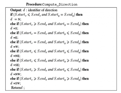
Considering that each node like S tries to reach a specific destination by starting the movement, its initial and final position can be displayed as S. start and S. end. With this method of displaying the movement path of a node, its movement direction (d) can also be determined. To calculate d for each node, the algorithm presented in Figure 3 is used.
Figure 3. Node direction pseudo code [33]
According to the definition of clustering, it can be simply said that clustering is gathering entities in groups with similar characteristics. In this paper, the cluster is referred to as a collection of similar track segments, such that the nodes within a cluster are close to each other in both spatial terms according to the distance measurement and have the same direction of movement (spatial direction). To create clusters, a path is simply divided into its constituent parts, then clustering is applied to those parts. Therefore, a single path can belong to multiple clusters based on the clusters of its segments.
Therefore, after determining the characteristics of each node, i.e., the direction of movement of the node's path, the k-means clustering algorithm is used to group similar path segments. The aim here is to present a new approach to enhance route clustering using the k-means algorithm by calculating the similarity of routes based on spatial distance and movement direction. Since the k-means algorithm seeks to minimize the average squared distance between points in the same cluster, the proposed approach also seeks to group paths that have similar movement patterns.
3.2 Select the cluster head
After the cluster is formed by the enhanced k-means algorithm, it is time to choose a cluster head node. The cluster head node plays an essential role in a cluster network. In fact, transmitters are responsible for data collecting, aggregating, and sending them to the base station. Cluster heads must be chosen with great care. And they should also have enough energy to send and collect data. The method of cluster head selection in wireless sensor networks significantly impacts network lifetime, communication overhead, network connectivity, load balancing, and network scalability. Choosing an appropriate cluster head selection method is crucial for achieving better energy efficiency, network performance, and overall system effectiveness in clustering-based routing protocols. On the other hand, the cluster heads should be placed in a position where the nodes can send their packets to them with the least energy consumption. Also, the location of the cluster head relative to the main station is important. If the cluster heads are not close to the main station, it causes the cluster heads to consume a lot of power to send their packets to the base station. As a result, the cluster heads soon run out of energy, which leads to network dispersion and eventual network death. In the suggested method for choosing a cluster head, three primary factors are considered. These variables include the node's remaining energy level, the distance between cluster members, and the distance between the nodes and the sink. How to choose the cluster head for defined cluster ‘C’ is described in Eq. (2). Based on this, the degree of fitness of each node in the cluster is determined, and it is evident that the node with the greatest degree of fitness (G) is elected as the cluster head.
$G=\max _{i \in C} \frac{R E_i}{D(i, B S)+\sum_{j \in G}\,\, D(i, j)}$ (2)
where, REi is the remained power of node i, D is the distance and BS is the base station.
The general framework of the proposed method is considered as the following steps:
1. Defining the initial simulation parameters.
2. Generating network nodes randomly.
3. Calculating the nodes' starting energy and the number of living nodes (the nodes whose energy has not been exhausted after sending the packet are called live nodes).
4. As long as the simulation time is not over or the number of live nodes is more than 1.5 times the number of clusters, the following steps are applied:
4.1. Determining the current position of the nodes (Node-Position) and the direction of movement of each node (Node-Direction).
4.2. Clustering of nodes based on the K-means algorithm.
4.3. Determining the cluster head for each cluster by calculating the fitness function (the fitness function determines the fitness level of each node according to the remaining energy of the node, the average distance of the node with the cluster members, and its distance with the base station. Then the node with the highest degree of fitness in each cluster is chosen as the head of the cluster.
4.4. At this stage, a packet is sent to the database for each live node.
4.5. Now, considering the point that the node may lose its energy after sending the packet, the living nodes try to move one step forward in their movement path, and again, the information of the network that is considered, i.e., the amount of residual energy and the number of live nodes.
5. If the simulation completion conditions are met, it will be finished(stop), otherwise, the above steps will be repeated.
In this article, MATLAB simulation is adopted to validate the efficiency of the suggested approach. In Table 1, the values of simulation parameters are presented.
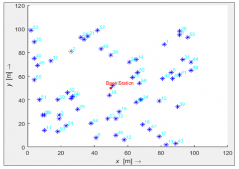
In a wireless sensor network, a certain number of nodes are randomly deployed in a geographical environment. These nodes are responsible for collecting environmental information. Each node must direct the collected environmental information to a central node called a sink or base station by sending information in a multi-hop method. The location of each node is random. Figure 4 illustrates the network structure that is randomly organized of several nodes along with the base station, which is considered a place to collect environmental data.
Table 1. Simulation parameters
|
Value |
Parameter |
|
1500 |
Simulation time (seconds) |
|
100*100 |
Simulation environment (square meters) |
|
50*50 |
Base station location |
|
80-120 |
Number of sensor nodes (number) |
|
800 |
Packet length (bits) |
|
0.5 |
The initial energy of the node(J) |
|
43 |
The neighborhood radius of the nodes |
|
5 |
The number of clusters |
Figure 4. A view of the network structure
In order to analyze the results and check the performance and efficiency of the proposed method, a comparison will be achieved with the basic paper method presented in Bavaghar et al. [34], with the name Energy Efficient Clustering Algorithm (EECA), and the Gaussian mixture clustering method. The number of active nodes and the remaining energy of the nodes are considered evaluation criteria.
4.1 Evaluation criteria
In wireless sensor networks, nodes usually face resource limitations, including the amount of energy of the nodes. Every sensor node should be able to save its energy as much as possible. Therefore, any algorithm presented in these networks should consider energy consumption considerations. As a result, it can be said that energy is the most important parameter for a node in a wireless sensor network and the evaluation of an algorithm presented in these networks. The amount of energy of each node is considered based on the total amount of power consumed by that node to receive the packet, plus the amount of energy consumed to identify the environment and listen to the channel, as well as the energy consumed to send the packet. Therefore, the amount of residual energy of the nodes as well as the number of live nodes in each round of simulation are evaluated. The energy dissipation value needs to be in a negligible range, minimizing energy dissipation is still desirable to maximize energy efficiency and prolong the network's operational lifetime. Overall, the focus is on understanding the energy dynamics and making informed decisions to improve the energy efficiency and performance of the network, while ensuring that the dissipated energy remains within an acceptable range.
Two different scenarios have been used to perform the evaluations. In the first scenario, the goal is to investigate the impact of the number of nodes on the efficiency of each of the compared methods. In this scenario, the number of nodes is chosen between 80 and 120 nodes. By changing the number of nodes, the evaluations were done again and the results of each of the compared methods are presented in the graph. By examining the graph of each method, the performance of each of them can be compared according to the parameters of energy consumption and remaining live nodes. The results of this scenario can be seen in Figures 5 and 6.
Figure 5. The sum of remaining energy for different numbers of nodes
Figure 6. Number of live nodes per different number of nodes
The findings in these graphs demonstrate that as the number of nodes increased, the quantity of energy left over and the total number of nodes continued to function throughout the experiment. The graphs illustrate a positive correlation between the number of nodes and two factors: the amount of remaining energy and the number of alive nodes during the experiment. Figure 5 shows that when the number of nodes increased, there is an observable increase in the quantity of energy that remained. This implies conserving more energy when the network size is large. Figure 6 shows when the total number of nodes increased, the number of alive nodes also increased.
The relationship between these two variables is positive, indicating that an increase in the total number of nodes is associated with a higher likelihood of nodes remaining operational. Given that each node might have more neighbors as the number of nodes rises, this seems evident. More neighbors imply more options for where to deliver packets to the sink. The number of neighbors grows as a consequence of the creation of multiple routes to the sink, which lessens the burden on each neighbor. As a result, the suggested strategy outperforms the comparison methods for both assessment criteria since it experiences better circumstances for both the residual energy and the number of live nodes than the compared approaches do.
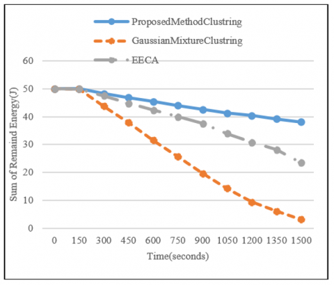
In the second scenario, the changes that occurred during the simulation period in the performance are investigated according to the evaluation parameters. Figures 7 and 8 show the results of this scenario.
Figure 7. The sum of remaining energy over the duration of the simulation
Figure 8. The number of live nodes during the simulation period
Examining the results of this scenario shows that with the passage of time, the residual energy of the network and the number of live nodes will decrease. It is clear that with the passage of time, the number of packets sent in the network increases, and the increase in the number of sent packets means an increase in energy consumption. The decrease in the residual energy of the network and the number of live nodes over time can be attributed to various factors: such as power consumption, battery life, or resource limitations within the network. As time goes on, the network and its nodes experience a decline in energy and operational capacity.
It is worth stating that in Figure 8, the number of live nodes during the simulation period is shown for the Gaussian Mixture Clustering result demonstrates a slow change in the final value. The explanation for this observation is as follows: i) Stable Cluster Formation: The slow change in the final value of live nodes suggests that the clustering algorithm forms relatively stable clusters. Once the clusters are formed, the nodes within each cluster tend to maintain their membership and continue functioning throughout the simulation period. The slow change indicates that there are minimal shifts or changes in the cluster composition or node participation over time; ii) Robustness and Consistency: The slow change in the final value of live nodes indicates that the cluster formation and node assignments are robust and consistent. This stability suggests that the clustering algorithm is effective in grouping nodes with similar characteristics and maintaining those groups throughout the simulation period.
However, in both evaluation criteria, as in the previous scenario, the proposed method performs better than the compared method. This scenario shows how far each of the compared methods has been able to keep the network more stable during the simulation period. The more energy remaining in the network during the simulation period, the more stable the network is. In this matter, the proposed approach shows that it has established the stability of the network more than the compared methods. The improvement of the proposed method compared to the Gaussian mixture clustering and EECA methods in both scenarios is summarized in Table 2.
Table 2. The improvement rate of the proposed method
|
Compared Methods |
Gaussian Clustering |
EECA |
|
|
Scenario 1 |
Alive Nodes |
64-82 |
1-3 |
|
Remained Energy(J) |
29.01-42.43 |
11.11-14.5 |
|
|
Scenario 2 |
Alive Nodes |
73 |
0-1 |
|
Remained Energy(J) |
34.92 |
14.61 |
|
With the emergence of new technologies, especially wireless sensor networks, many researchers have shown interest in this subject due to the industrial and commercial attractiveness of this field. Therefore, this research area has been raised as one of the important research areas in recent years. In these networks, one of the most basic parameters is to maintain the energy of the nodes in the sensor network. Therefore, providing an approach that can reduce energy consumption as much as possible while maintaining network service quality parameters still seems to be a challenging research topic. In this research, an approach for clustering wireless sensor networks is proposed using the K-means algorithm and a new cluster head selection method. The proposed hybrid approach clusters sensor nodes in a way that saves energy.
For evaluation purposes, the suggested approach is compared with the Gaussian mixture clustering and EECA methods using MATLAB programming language. Also, in order to measure the performance of the proposed method, two scenarios of variable number of nodes and duration of simulation have been used. The results of the evaluations, which are presented in the form of two parameters, the remaining energy of the nodes and the number of remaining live nodes, show that the suggested approach has provided better results than the compared methods.
Due to the exceptional expansion of IoT sensor network applications, it seems that this research and business field is still interested in various research challenges. In the future, it can further extend this research by presenting new approaches using evolutionary hybrid algorithms such as bat, lion hunting, firefly, or harmony search for clustering and optimizing route selection.
[1] Arora, V.K., Sharma, V., Sachdeva, M. (2016). A survey on LEACH and other’s routing protocols in wireless sensor network. Optik, 127(16): 6590-6600. https://doi.org/10.1016/j.ijleo.2016.04.041.
[2] Ahmad, I.A., Al-Nayar, M.M.J., Mahmood, A.M. (2022). Investigation of energy efficient clustering algorithms in WSNs: A review. Mathematical Modelling of Engineering Problems, 9(6): 1693-1703. https://doi.org/10.18280/mmep.090631
[3] Al-Hilfi, H.I.M., Al-Nayar, M.M.J. (2022). Increase the WSN-lifespan used in monitoring forest fires by PSO. Mathematical Modelling of Engineering Problems, 9(3): 583-590. https://doi.org/10.18280/mmep.090304
[4] Ramson, S.J., Moni, D.J. (2017). Applications of wireless sensor networks—A survey. In 2017 International Conference on Innovations in Electrical, Electronics, Instrumentation and Media Technology (ICEEIMT), pp. 325-329. https://doi.org/10.1109/ICIEEIMT.2017.8116858
[5] Nasser, A.R., Mahmood, A.M. (2021). Cloud-based Parkinson’s disease diagnosis using machine learning. Mathematical Modelling of Engineering Problems, 8(6): 915-922. https://doi.org/10.18280/mmep.080610
[6] Abdulaziz, W.B., Croock, M.S. (2022). Design of smart irrigation system for vegetable farms based on efficient wireless sensor network. Iraqi Journal of Computers, Communications, Control and Systems Engineering, 22(1): 72-85.
[7] Hashim, S.A., Jawad, M.M., Wheedd, B. (2020). Study of energy management in wireless visual sensor networks. Iraqi Journal of Computers, Communications, Control and Systems Engineering, 20(1): 68-75.
[8] Hamza, E.K., Al-asady, H.H. (2017). Indoor localization system using wireless sensor network. Iraqi Journal of Computers, Communications, Control and Systems Engineering, 18(1): 29-38.
[9] Kandris, D., Nakas, C., Vomvas, D., Koulouras, G. (2020). Applications of wireless sensor networks: An up-to-date survey. Applied System Innovation, 3(1): 14. https://doi.org/10.3390/asi3010014
[10] Khalaf, O.I., Sabbar, B.M. (2019). An overview on wireless sensor networks and finding optimal location of nodes. Periodicals of Engineering and Natural Sciences (PEN), 7(3): 1096-1101. https://doi.org/10.1166/jctn.2019.8134
[11] Xu, L., Collier, R., O’Hare, G.M. (2017). A survey of clustering techniques in WSNs and consideration of the challenges of applying such to 5G IoT scenarios. IEEE Internet of Things Journal, 4(5): 1229-1249. https://doi.org/10.1109/JIOT.2017.2726014
[12] Shahraki, A., Taherkordi, A., Haugen, Ø., Eliassen, F. (2020). Clustering objectives in wireless sensor networks: A survey and research direction analysis. Computer Networks, 180: 107376. https://doi.org/10.1016/j.comnet.2020.107376
[13] Wohwe Sambo, D., Yenke, B.O., Förster, A., Dayang, P. (2019). Optimized clustering algorithms for large wireless sensor networks: A review. Sensors, 19(2): 322. https://doi.org/10.3390/s19020322
[14] Amutha, J., Sharma, S., Sharma, S.K. (2021). Strategies based on various aspects of clustering in wireless sensor networks using classical, optimization and machine learning techniques: Review, taxonomy, research findings, challenges and future directions. Computer Science Review, 40: 100376. https://doi.org/10.1016/j.cosrev.2021.100376
[15] Wang, J., Gao, Y., Wang, K., Sangaiah, A.K., Lim, S.J. (2019). An affinity propagation-based self-adaptive clustering method for wireless sensor networks. Sensors, 19(11): 2579. https://doi.org/10.3390/s19112579
[16] Mohan, P., Subramani, N., Alotaibi, Y., Alghamdi, S., Khalaf, O.I., Ulaganathan, S. (2022). Improved metaheuristics-based clustering with multihop routing protocol for underwater wireless sensor networks. Sensors, 22(4): 1618. https://doi.org/10.3390/s22041618
[17] Kim, D.S., Chung, Y.J. (2006). Self-organization routing protocol supporting mobile nodes for wireless sensor network. In First International Multi-Symposiums on Computer and Computational Sciences (IMSCCS'06), 2: 622-626. https://doi.org/10.1109/IMSCCS.2006.265
[18] Ali, S., Madani, S.A., Khan, I.A. (2014). Routing protocols for mobile sensor networks: A comparative study. arXiv preprint arXiv: 1403:3162. https://doi.org/10.48550/arXiv.1403.3162
[19] Sara, G.S., Sridharan, D. (2014). Routing in mobile wireless sensor network: A survey. Telecommunication Systems, 57: 51-79. https://doi.org/10.1007/s11235-013-9766-2
[20] Nayebi, A., Sarbazi-Azad, H. (2011). Performance modeling of the LEACH protocol for mobile wireless sensor networks. Journal of Parallel and Distributed Computing, 71(6): 812-821. https://doi.org/10.1016/j.jpdc.2011.02.004
[21] Peng, L., Xu, J.B. (2009). ECDGA: An energy-efficient cluster-based data gathering algorithm for mobile wireless sensor networks. In 2009 International Conference on Computational Intelligence and Software Engineering, pp. 1-4. https://doi.org/10.1109/CISE.2009.5366773
[22] Olascuaga-Cabrera, J.G., Lopez-Mellado, E., Ramos-Corchado, F. (2009). Self-organization of mobile devices networks. In 2009 IEEE International Conference on System of Systems Engineering (SoSE), pp. 1-6.
[23] Sara, G.S. (2010). Energy efficient clustering and routing in mobile wireless sensor network. arXiv preprint arXiv: 1011.5326. https://doi.org/10.48550/arXiv.1011.5326
[24] Lohani, R.B., Singh, V. (2019). Mobility aware energy efficient clustering for wireless sensor network. In 2019 IEEE International Conference on Electrical, Computer and Communication Technologies (ICECCT).
[25] Masdari, M., Barshande, S., Ozdemir, S. (2019). CDABC: chaotic discrete artificial bee colony algorithm for multi-level clustering in large-scale WSNs. The Journal of Supercomputing, 75: 7174-7208. https://doi.org/10.1007/s11227-019-02933-3
[26] Deng, S., Li, J., Shen, L. (2011). Mobility-based clustering protocol for wireless sensor networks with mobile nodes. IET Wireless Sensor Systems, 1(1): 39-47. https://doi.org/10.1049/iet-wss.2010.0084
[27] Neamatollahi, P., Naghibzadeh, M. (2018). Distributed unequal clustering algorithm in large-scale wireless sensor networks using fuzzy logic. The Journal of Supercomputing, 74: 2329-2352. https://doi.org/10.1007/s11227-018-2261-5
[28] Wang, N., Chen, D., Chen, J., Xu, X., Wan, J. (2018). Clustering data gathering method based on compressed sensing in wireless sensor networks. In 2018 10th International Conference on Intelligent Human-Machine Systems and Cybernetics (IHMSC), 2: 214-217. https://doi.org/10.1109/IHMSC.2018.10155
[29] Frahling, G., Sohler, C. (2006). A fast k-means implementation using coresets. In Proceedings of the twenty-second annual symposium on Computational geometry, pp. 135-143. https://doi.org/10.1145/1137856.1137879
[30] Arthur, D, Vassilvitskii, S. (2007). k-means++: The advantages of careful seeding. In: SODA ’07: Proceedings of the eighteenth annual ACM-SIAM symposium on discrete algorithms. Philadelphia, PA, USA: Society for Industrial and Applied Mathematics, pp. 1027-1035.
[31] Hailin, C., Xiuqing, W., Junhua, H. (2007). Adaptive k-means clustering algorithm, MIPPR. Pattern Recognition and Computer Vision.
[32] Lee, J.G., Han, J., Whang, K.Y. (2007). Trajectory clustering: A partition-and-group framework. In Proceedings of the 2007 ACM SIGMOD international conference on Management of data, pp. 593-604. https://doi.org/10.1145/1247480.1247546
[33] Ossama, O., Mokhtar, H.M., El-Sharkawi, M.E. (2011). An extended k-means technique for clustering moving objects. Egyptian Informatics Journal, 12(1): 45-51. https://doi.org/10.1016/j.eij.2011.02.007
[34] Bavaghar, M., Mohajer, A., Motlagh, S.T. (2020). Energy efficient clustering algorithm for wireless sensor networks. Proceeding 2017 International Conference Wireless Communication Signal Processing Networking, 7(4): 238-247. https://doi.org/10.7508/jist.2019.04.001