Kaliyaperumal Chinnadurai![]() | Singaram Athithan*
| Singaram Athithan*![]()
© 2023 IIETA. This article is published by IIETA and is licensed under the CC BY 4.0 license (http://creativecommons.org/licenses/by/4.0/).
OPEN ACCESS
In this research work, a mathematical model for exploring the dynamics of poverty and drug addiction among human population is developed and analyzed by the way of deterministic and stochastic differential equations. Our model is constructed by assuming four compartments of the population namely non-impoverished or rich people, poor people, drug addicts and recovered people population. The model exhibits three equilibrium points and stability of those equilibrium points are analyzed in detail. To enhance and validate the analysis of solutions and equilibrium points, it has been carried out numerical simulation which will also shows the effectiveness of our model. We tried to depict the effect of drug addiction and poverty in society through our mathematical model has some occasions explained through suitable numerical explanations by plotting the respective compartments. We hope our suggestions may serve in a better manner for the future to reduce the poor people.
poverty, drug addiction, stability, stochastic model, numerical simulation, intervention
Nowadays directly goes to addict the young and moderate drug used people. They are not recovered quickly from drug usage after they have recovered under the proper guidelines and counseling in particular periods. The poverty/poor people may contact drug-addicted people, who are also easily addicted to drug usage and then face so many struggles in daily life and run in regular life.
Currently, endemic research is getting more and more grounded in reality thanks to societal issues. Based on the association between poverty and drug addiction. So, we are beginning to create mathematical models.
“Drug dependence must be treated primarily as a disease and not a crime. Countries increasingly realize the benefits of drug treatment for not only individuals themselves but also for society and the economy [1]”.
Only a small number of samples of mouth fluid were required. Compared to the traditional ELISA test, this sensing approach improves the sensitivity and specificity of ketamine analysis. Additionally, when resources are limited, the dissection is carried out using a smart phone app that does not require expensive equipment. In addition to ketamine, the cP-ELISA sensing system provides a high-quality, quick-testing platform that uses amphetamines, cocaine, and opioids [2].
Drug abuse has been one of the biggest problems for governments everywhere. Risky injectables and sexual contact among drug users are grave public health issues because the danger of transmission of blood-borne infections includes HIV, HCV, and HBV, particularly among the underprivileged and most at-risk groups.
On top two misused drugs in Taiwan, according to medical institutes, continue to be historically abused substances like heroin and methamphetamine. On the other side, throughout time, the number of people who take new drugs like ketamine has progressively increased, and MDMA abuse has returned [3].
The Joint UNODC-WHO initiative closely connects with the WHO's Mental Health Gap Action Programme (mhGAP) was established in November 2008 to develop solutions for scaling up mental, neurological, and drug use disorder treatment. One of the eight priority conditions is disorders caused by illegal drug use [4].
The joint UNODC-WHO programme:
Leads a global collaborative effort to improve drug use disorder treatment and care coverage and quality in low- and middle-income nations.
Promotes the development of comprehensive and integrated treatment programmes that may link local, state, and federal agencies to offer drug addicts a continuum of care.
Maps are regional needs, governing laws, and available resources and programmes for drug addiction treatment.
Supports revisions to policy and law to achieve drug policy balance and promote compassionate and effective drug prevention, treatment, and care.
Improves exposure in rural and isolated locations by developing low-cost outreach care and treatment services.
The prevention, rehabilitation, and treatment of drug use disorders are incorporated into the conventional healthcare system as a built-in component of the integrated healthcare continuum, working with NGOs to ensure perfect cooperation with the healthcare system.
Supports local networks of top-notch service providers that are devoted to social services, HIV/AIDS prevention, and treatment [4].
Prostitution is the street link to poverty. Female prostitutes recognize as members of racial and ethnic minorities who are poor, uneducated and have a dear of marketable skills. Legislators have chastised and continue to condemn these ladies because they view them as wicked persons. However, consistency in implementing prostitution laws, including laws prohibiting patronizing prostitutes, has been and is inequitable [5].
Tobacco contains a very addictive substance called nicotine. Use of tobacco products may increase the chance of developing heart and lung ailments, more than 20 different kinds or subtypes of cancer, and a wide range of other life-altering illnesses [6].
Even non-smokers can die from tobacco use. And also linked to the poor health consequences, second-hand smoke exposure accounts for over 1.2 million yearly fatalities. Nearly half of all youngsters breathe tobacco smoke-polluted air, and 65 000 young people pass away from diseases each year linked to second-hand smoke. Smoking during pregnancy may result in long-term health issues for the unborn child [6].
It has been determined by experts from all fields, including sociologists and economists, that poverty and crime have an "intimate" connection. World Bank and the United Nations see crime as the primary barrier to a country's development. Governments coping with the effects of poverty usually have to deal with the problem of crime as they work to develop their nation's economy and society. Uncertainty and instability are made by crime, making it difficult for companies to thrive(at micro and macroeconomic levels) [7-9].
Heavy drinking links to an increased risk of cancer. Fatty liver disease and cirrhosis are two conditions that can result from it. The brain and other organs may be potentially harmed by drinking. During pregnancy, liquor might be harmful to your baby. Alcohol also raises the chances of dying in vehicle accidents, illnesses, homicides, and suicides [10, 11].
Changes such as increased rainfall, for example, will impact African dry lands and thus increase the burden of vector-borne water-related diseases in regions already vulnerable to poverty [12].
Sakib et al. [13] they have planned five compartments. but now we have simplified in our model into four compartment.
In this paper is organized as follows: Section 2 portrayed the basic model and analysis which comprises the subsections as basic reproduction number, equilibria and their stability analysis. Section 3 describes the Stochastic Model, section 4 as we display the numeric results and simulating the design of Python showing the figure of numerical simulation on the deterministic model and stochastic model. At the last, we have given our conclusion in section 5.
We designed and analyzed a non-linear model for poverty and drug addiction by dividing the whole population into 4 different compartments. The age of adults is primarily involved in drug addiction [14]. Based on this, we have taken into account the age group's population that is affected by poverty.
Let H(t), D(t), P(t) and R(t) be the fractions of the High class/Non-Impoverished, the Drug Addiction individuals and the Poverty individuals in the population and Recovered population respectively, at time t. It is assumed that the total population is varying and homogeneously mixed [15, 16].
The model assumptions are as follows:
α1 indicates the rate of migration of non-impoverished class into the drug-using population, which is influenced by the unemployment and underemployment rates and, typically, directly correlated with poverty.
β shows how quickly people in the non-impoverished class move into the impoverished or poor class.
γ is the frequency of recruitment of an addict into the poverty class.
α2 and α3 are recovered individual to drug addiction and poor people by the help of some kind of NGO's provide poverty people necessity and rehabilitation at reduced rates of drug addiction to given the counseling.
The term $\alpha_1 H \frac{D}{N}$ reflects the rate at which high class users become drug addicts, where the transmission rate is α1.
Similarly the term $\alpha_2 P \frac{D}{N}$ reflects the rate of interaction between the drug addiction and poverty classes, where the transmission rate is α2.
μ is natural death rate.
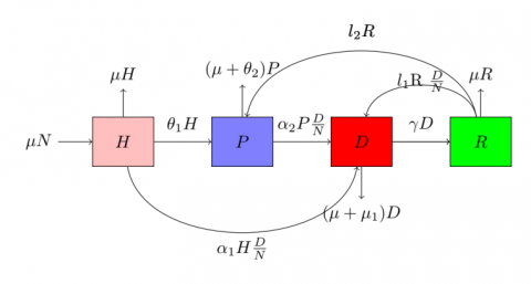
The ODE model equation framed as follows in Figure 1 and the parameter descriptions are given the Table 1:
Figure 1. Model flow diagram
Table 1. Description of parameters
|
Parameter |
Description |
|
l1 |
The rate at which people move from a recovery class to a drug addiction class |
|
l2 |
After a period of recovery, the rate of people who enter the poor class |
|
μ |
Natural birth rate/mortality rate |
|
μ1 |
Due to heavy drug use, the mortality rate |
|
θ1 |
A rate of an incurable disease that infects people |
|
θ2 |
Rate of progression from Non-impoverished to Poverty population |
|
α1 |
The rate of flow from the high/wealthy class to the drug class by drug addiction |
|
α2 |
The rate of flow from poor class to drug class by the addiction |
|
γ |
Rate of drug addicted people recruited into rehabilitation |
$\begin{gathered}\frac{d H}{d t}=\mu N-\left(\mu+\theta_1\right) H-\alpha_1 H \frac{D}{N} \\ \frac{d P}{d t}=\theta_1 \mathrm{H}-\left(\mu+\theta_2\right) \mathrm{P}-\alpha_2 \mathrm{P} \frac{\mathrm{D}}{\mathrm{N}}+\mathrm{l}_2 \mathrm{R} \\ \frac{d D}{d t}=\alpha_1 \mathrm{H} \frac{\mathrm{D}}{\mathrm{N}}+\alpha_2 \mathrm{P} \frac{\mathrm{D}}{\mathrm{N}}-\left(\gamma+\mu+\mu_1\right) \mathrm{D}+\mathrm{l}_1 \mathrm{R} \frac{\mathrm{D}}{\mathrm{N}} \\ \frac{d R}{d t}=\gamma D-\mathrm{l}_1 \mathrm{R} \frac{\mathrm{D}}{\mathrm{N}}-\mathrm{l}_2 \mathrm{R}-\mu \mathrm{R}\end{gathered}$ (1)
The above system (1) has simplified as follows:
$\begin{gathered}\frac{d H}{d t}=\mu N-\left(\mu+\theta_1\right) H-\alpha_1 H \frac{D}{N} \\ \frac{d P}{d t}=\theta_1 \mathrm{H}-\left(\mu+\theta_2\right) \mathrm{P}-\alpha_2 \mathrm{P} \frac{\mathrm{D}}{\mathrm{N}}+\mathrm{l}_2 \mathrm{R} \\ \frac{d D}{d t}=\alpha_1 \mathrm{H} \frac{\mathrm{D}}{\mathrm{N}}+\alpha_2 \mathrm{P} \frac{\mathrm{D}}{\mathrm{N}}-(\mathrm{k}) \mathrm{D}+\mathrm{l}_1 \mathrm{R} \frac{\mathrm{D}}{\mathrm{N}} \\ \frac{d R}{d t}=\gamma D-\mathrm{l}_1 \mathrm{R} \frac{\mathrm{D}}{\mathrm{N}}-\mathrm{l}_2 \mathrm{R}-\mu \mathrm{R}\end{gathered}$ (1a)
where, $\mathrm{N}=\mathrm{H}+\mathrm{P}+\mathrm{D}+\mathrm{R}$ and $k=\gamma+\mu+\mu_1$.
2.1 Existence of equilibria
Our model equilibrium points are identified by the setting of right hand side of the model (1) to zero [15]. The system (1) has equilibria shown below:
(i) Both drug addiction and poverty free equilibrium $E_0\left(\frac{H^0}{N}, 0,0,0\right)=\left(\frac{\mu}{\mu+\theta_1}, 0,0,0\right)$.
(ii) Poverty Free Equilibrium (PFE) $E_1\left(\frac{H^1}{N}, 0, \frac{D^1}{N}, \frac{R^1}{N}\right)=$ $\left(\frac{\mu}{\left(\mu+\theta_1+\alpha_1 x\right)}, 0, x^1, \frac{\gamma x}{\left(l_1 x+l_2+\mu\right)}\right)$, where, $\mathrm{x}^1=\frac{\mathrm{kD}}{\alpha_1 H+l_1 \mathrm{R}}$, and
(iii) Endemic Equilibrium (EE) $\$ E_2\left(\frac{H^*}{N}, \frac{p^*}{N}, \frac{D^*}{N}, \frac{R^*}{N}\right)$,
where,
$\begin{gathered}\frac{H^*}{N}=\frac{\mu}{\mu+\theta_1+\alpha_1 \mathrm{x}}, \\ \frac{P^*}{N}=\frac{\mathrm{k}-\frac{l_1 \mathrm{R}}{\mathrm{N}}-\frac{\alpha_1 \mathrm{H}}{\mathrm{N}}}{\alpha_2}, \\ \frac{D^*}{N}=x, \\ \frac{R^*}{N}=\frac{\gamma \mathrm{x}}{\mathrm{l}_1 \mathrm{x}+\mathrm{l}_2+\mu}\end{gathered}$
where, $x=\alpha_1 x^3+\alpha_2 x^2+\alpha_3 x-\alpha_4$.
Here,
$\begin{aligned} & a_1=\alpha_2 \alpha_1 l_1, \\ & a_2=l_1 \alpha_1(k-\gamma)+\alpha_2 l_1\left(\mu+\theta_1\right)+\alpha_1 \alpha_2\left(l_2+\mu-l_1-\gamma\right) \\ & a_3=\alpha_2 \mu\left(l_2+\mu+\theta_1-\alpha_1+\gamma\right)+l_1 \theta_1\left(k-\alpha_2-\gamma\right)+ \\ & l_1 \mu\left(\mathrm{kx}-\alpha_1-\gamma\right)+l_2 \alpha_2\left(\theta_1-\alpha_1\right)+k \alpha_1\left(l_2+\mu\right)+ \\ & \alpha_2 \theta_1 \gamma, \\ & a_4=\alpha_2\left(\mu\left(l_2+\mu+\theta_1\right)+l_2 \theta_1\right)-\mu\left(\alpha_2-\alpha_1\right)\left(l_2+\right. \\ & \left.\mu)-k\left(\mu\left(l_2+\mu+\theta_1\right)+l_2 \theta_1\right)\right] .\end{aligned}$
We have to consider the one positive root case only by numerically.
2.2 Stability analysis
2.2.1 Stability analysis of poverty free equilibrium
Theorem 2.1
The PFE E1 is locally asymptotically stable.
Proof.
To study the stability of the variational matrix M1 of the system corresponding to PFE E1 is obtained as:
$M_1=\left(\begin{array}{cccc}p_{11} & 0 & p_{13} & 0 \\ p_{21} & p_{22} & 0 & p_{24} \\ p_{31} & p_{32} & p_{33} & p_{34} \\ 0 & 0 & p_{43} & p_{44}\end{array}\right)$
where,
$\begin{array}{ll}p_{11}=-\left(\mu+\theta_1\right)-\alpha_1 \frac{D}{N}, & p_{13}=-\frac{\alpha_1 H}{N}, \\ p_{22}=-\left(\mu+\theta_2\right)-\frac{\alpha_2 D}{N}, & p_{21}=\theta_1 \\ p_{24}=l_2, & p_{31}=\frac{\alpha_1 D}{N}, \\ p_{33}=\alpha_1 \frac{H}{N}-k+l_1 \frac{R}{N}, & p_{32}=\alpha_2 \frac{D}{N},\\ p_{34}=l_1 \frac{D}{N}, & p_{43}=\gamma-l_1 \frac{R}{N}, \\ p_{44}=-l_2-\mu-l_1 \frac{D}{N} . & \end{array}$
The eigenvalues are given by the roots of the following characteristic equation in λ.
$\lambda^4+\mathrm{p}_1 \lambda^3+\mathrm{p}_2 \lambda^2+\mathrm{p}_3 \lambda+\mathrm{p}_4=0$
where,
$\begin{gathered}p_1=-\left(p_{11}+p_{22}+p_{33}+p_{44}\right), \\ p_2=\left[p_{11}\left(p_{22}+p_{33}+p_{44}\right)+p_{22}\left(p_{33}+p_{44}\right)+p_{33} p_{44}\right. \left.+p_{13} p_{31}\right], \\ p_3=\left[-p_{11} p_{22}\left(p_{33}+p_{44}\right)-\left(p_{33} p_{44}\right)\left(p_{11}+p_{22}\right)\right. -p_{13} p_{31}\left(p_{22}+p_{44}\right) \left.-p_{32}\left(p_{13} p_{21}+p_{24} p_{43}\right)\right], \\ p_4=\left[p_{11} p_{22}\left(p_{33} p_{44}-p_{44} p_{31}\right)+p_{11} p_{32} p_{24} p_{43}\right. \left.+p_{13} p_{21} p_{44} p_{32}\right] .\end{gathered}$
By Routh Hurwitz criteria, roots of the bi-quadratic equation will have negative real parts is positive. Now $p_1>0$, $p_3>0, p_4$ and $p_1 p_2 p_3>p_3^2+p_1^2 p_4$.
Hence the equilibrium point $E_1$ is locally asymptotically stable [17].
2.2.2 Stability analysis of endemic equilibrium
Theorem 2.2
The EE E2 is locally asymptotically stable.
Proof.
The variational matrix, M corresponding to E2 is given by:
$M=\left(\begin{array}{cccc}e_{11} & 0 & e_{13} & 0 \\ e_{21} & e_{22} & e_{23} & e_{24} \\ e_{31} & e_{32} & e_{33} & e_{34} \\ 0 & 0 & e_{43} & e_{44}\end{array}\right)$
where,
$\begin{aligned} e_{11}=-\left(\mu+\theta_1\right)-\alpha_1 \frac{\mathrm{D}}{\mathrm{N}}, \\ \mathrm{e}_{13}=-\alpha_1 \frac{\mathrm{H}}{\mathrm{N}}, \\ e_{21}=\theta_1, \\ \mathrm{e}_{22}=-\left(\mu+\theta_2\right)-\frac{\alpha_2 D}{N}, \\ e_{23}=-\alpha_2 \frac{P}{N}, \\ e_{24}=l_2, \\ e_{31}=\alpha_1 \frac{D}{N}, \\ e_{32}=\alpha_2 \frac{D}{N},\end{aligned}$
$\begin{gathered}e_{33}=\alpha_1 \frac{H}{N}+\frac{\alpha_2 P}{N}-k+l_1 \frac{R}{N}, \\ e_{34}=l_1 \frac{D}{N}, \\ e_{43}=\gamma-l_1 \frac{R}{N}, \\ e_{44}=-l_2-\mu-l_1 \frac{D}{N} .\end{gathered}$
The eigenvalues are given by the roots of the following characteristic equation in λ.
$\lambda^4+e_1 \lambda^3+e_2 \lambda^2+e_3 \lambda+e_4=0$
where,
$\begin{gathered}e_1=-\left(e_{11}+e_{12}+e_{13}+e_{14}\right), \\ e_2=e_{11}\left(e_{22}+e_{33}+e_{-44}\right)+e_{22}\left(e_{33}+e_{44}\right)-p_{34} p_{43} \\ -p_{32} p_{-} 23, \\ e_3=-e_{11} e_{22}\left(e_{33}+e_{44}\right)+\left(e_{34} e_{43}-e_{33} e_{44}\right)\left(e_{11}+e_{22}\right) \\ +e_{32} e_{23}\left(e_{11}+e_{44}\right)-e_{32}\left(e_{24} e_{43}\right. \\ \left.+e_{21} e_{32}\right)+e_{13} e_{31} e_{22}, \\ e_4=e_{11} e_{22}\left(e_{33} e_{44}-e_{34} e_{43}\right)+e_{11} e_{32}\left(e_{24} e_{43}-e_{23} e_{44}\right) \\ +e_{13} e_{44}\left(e_{21} e_{32}-e_{31} e_{22}\right) .\end{gathered}$
By Routh Hurwitz criteria, roots of the bi-quadtratic equation will have negative real parts is positive.
Therefore,
$e_1>0, e_3>0, e_4>0$ and $e_1 e_2 e_3>e_3^2+e_1^2 e_4$.
Hence, the equilibrium point E2 is locally asymptotically stable.
In this section, we extend our deterministic model to a stochastic model because the issue of drug addiction may be detected more accurately using stochastic models. Based on the method's assumptions, an SDE (Stochastic Differential Equation) model is derived [18-21]. Let X(t)=(X1(t), X2(t), X3(t), X4(t))T be a continuous random variable for (H(t), P(t), D(t), R(t))T and T means the transpose of a matrix.
Let $\Delta X=X(t+\Delta t)-X(t)=\left(\Delta X_1, \Delta X_2, \Delta X_3, \Delta X_4\right)^T$ signify the random vector for the change in random variables during time interval $\Delta t$. Here, we'll create the transition maps for the SDE model, which outline all relevant transitions between states. Based on our ODE model system (1), we can see that the exist 12 possibilities between the states during the small interval $\Delta t$. We are discussed the state changes and their probabilities in Table 2.
Let us consider the case the recruitment of drug addictions becomes high class / poverty and drug addiction. In this case, the state change $\Delta X$ denotes by $\Delta X=(1,0,0,0)$ its probability of the change is given by:
$\begin{gathered}\operatorname{Prob}\left(\Delta X_1, \Delta X_2, \Delta X_3, \Delta X_4\right)= \\ (1,0,0,0) \mid\left(X_1, X_2, X_3, X_4\right)=P_1=\mu N \Delta t+o(\Delta t) .\end{gathered}$
One will rapidly to solve the expectation change $E(\Delta X)$ and its covariance matrix $V(\Delta X)$ connected with $\Delta X \mathrm{b}$ ignoring the terms higher than $o(\Delta t)$. The expectation of $\Delta X$ is given by:
$E(\Delta X)=\sum_{\mathrm{i}=1}^{12} \mathrm{P}_{\mathrm{i}}(\Delta \mathrm{X})_{\mathrm{i}} \Delta \mathrm{t}=\left(\begin{array}{c}\mu N-\left(\mu+\theta_1\right) X_1-\alpha_1 X_1 \frac{X_3}{N} \\ \theta_1 X_1-\left(\mu+\theta_2\right) X_2-\alpha_2 X_2 \frac{X_3}{N}+l_2 X_4 \\ \alpha_1 X_1 \frac{X_3}{N}+\alpha_2 X_2 \frac{X_3}{N}-\mathrm{kX}_3+l_1 X_4 \frac{X_3}{N} \\ \gamma X_3-l_1 X_4 \frac{X_3}{N}-l_2 X_4-\mu X_4\end{array}\right) \Delta t=f\left(X_1, X_2, X_3, X_4\right) \Delta t$ (2)
Here, the ODE system (1) can be noted that the expectation vector and the function f are in the same form. Since,
$\begin{gathered}\mathrm{V}(\Delta \mathrm{X})=\mathrm{E}\left((\Delta \mathrm{X})(\Delta \mathrm{X})^{\mathrm{T}}\right)-\mathrm{E}(\Delta \mathrm{X})\left(\mathrm{E}(\Delta \mathrm{X})^{\mathrm{T}}\right) \\ \text { and } E\left((\Delta X)(\Delta X)^T\right)=f(X)\left(f(X)^T\right) \Delta t\end{gathered}$
Table 2. The probability of possible states and changes
|
Possible change of states |
|
Probability of change of state |
|
(ΔX)1 =(1, 0, 0, 0)T |
Change when the recruitment growth |
$P_1=\mu N \Delta t+o(\Delta t)$ |
|
(ΔX)2 =(-1, 0, 0, 0)T |
Change when the natural death |
$P_2=\mu X_1 \Delta t+o(\Delta t)$ |
|
(ΔX)3 =(-1, 1, 0, 0)T |
Change when the high class to poor people growth rate |
$P_3=\theta_1 X_1 \Delta t+o(\Delta t)$ |
|
(ΔX)4 =(-1, 0, 1, 0)T |
Change when the high class to drug addicted people growth rate |
$P_4=\alpha_1 X_1 \frac{X_3}{N} \Delta t+o(\Delta t)$ |
|
(ΔX)5 =(0, -1, 0, 0)T |
Change when the poor people death rate and natural disaster affected |
$P_5=\left(\mu+\theta_2\right) X_2 \Delta t+o(\Delta t)$ |
|
(ΔX)6 =(0, -1, 1, 0)T |
Change when the poor people to drug addicted peoples are interaction to total population |
$P_6=\left(\alpha_2 X_3 X_2\right) / N \Delta t+o(\Delta t)$ |
|
(ΔX)7 =(0, 1, 0, -1)T |
Change when the recovered peoples move to poor population |
$P_7=l_2 X_4 \Delta t+o(\Delta t)$ |
|
(ΔX)8 =(0, 0, -1, 1)T |
Change when the drug addicted population goes to recovery population due to guidelines |
$P_8=\gamma X_3 \Delta t+o(\Delta t)$ |
|
(ΔX)9 =(0, 0, -1, 0)T |
Change when the drug addicted population natural and disease death rate |
$P_9=\left(\mu+\mu_1\right) X_3 \Delta t+o(\Delta t)$ |
|
(ΔX)10 =(0, 0, 1, -1)T |
Changed into recovered and drug addicted people interact with total population growth |
$P_{10}=\frac{l_1 X_4 X_3}{N} \Delta t+o(\Delta t)$ |
|
(ΔX)11 =(0, 0, 0, -1)T |
Change into the natural death rate after recovery |
$P_{11}=\mu X_4 \Delta t+o(\Delta t)$ |
|
(ΔX)12 =(0, 0, 0, 0)T |
No Change |
$P_{12}=1-\sum_{i=1}^{12} P_i+o(\Delta t)$ |
It can be approximately diffusion matrix $\mathrm{V}$ times $\Delta t$ by neglecting the term of $(\Delta t)^2$ such that $V(\Delta X) \approx$ $E\left((\Delta X)(\Delta X)^T\right)$
Hence,
$E\left((\Delta X)(\Delta X)^T\right)=\sum_{i=1}^{12} P_i\left((\Delta X)_i(\Delta X)_i^T\right) \Delta t=\left(\begin{array}{cccc}V_{11} & V_{12} & V_{13} & 0 \\ V_{21} & V_{22} & V_{23} & V_{24} \\ V_{31} & V_{32} & V_{33} & V_{34} \\ 0 & V_{42} & V_{43} & V_{44}\end{array}\right) \cdot \Delta \mathrm{t}=\Omega \cdot \Delta \mathrm{t}$ (3)
where, we solved the above diffusion matrix is symmetric, positive-definite and each component of this 4 x 4 matrix can be attained as follows:
$\begin{array}{cc} V_{11}=P_1+P_2+P_3+P_4, & V_{14}=V_{41}=0, \\ V_{22}=P_3+P_5+P_6+P_7, & V_{24}=V_{42}=-P_7 . \\ V_{33}=P_4+P_6+P_8+P_9+P_{10}, & V_{12}=V_{21}=-P_3, \\ V_{44}=P_7+P_8+P_{10}+P_{11} . & V_{23}=V_{32}=-P_6, \\ V_{13}=V_{31}=-P_4, & V_{34}=V_{43}=-P_8 . \end{array}$
We are following the approach considered in the research [18] and construct a matrix M such that V=MMT, where M is a 4 x 10 matrix.
$\mathrm{M}=\left(\begin{array}{cccccccccc}\mathrm{m}_{101} & \mathrm{~m}_{102} & \mathrm{~m}_{103} & 0 & 0 & 0 & 0 & 0 & 0 & 0 \\ 0 & \mathrm{~m}_{202} & 0 & \mathrm{~m}_{204} & \mathrm{~m}_{205} & \mathrm{~m}_{206} & 0 & 0 & 0 & 0 \\ 0 & 0 & \mathrm{~m}_{303} & 0 & \mathrm{~m}_{305} & 0 & \mathrm{~m}_{307} & \mathrm{~m}_{308} & \mathrm{~m}_{309} & 0 \\ 0 & 0 & 0 & 0 & 0 & \mathrm{~m}_{406} & \mathrm{~m}_{407} & 0 & \mathrm{~m}_{409} & \mathrm{~m}_{410}\end{array}\right)$
where,
$\begin{aligned} m_{101} & =\sqrt{\mu N-\mu X_1}, & m_{305} & =\sqrt{\alpha_2 X_2 \frac{X_3}{N},} \\ m_{102} & =-\sqrt{\theta_1 X_1}, & m_{307} & =-\sqrt{\gamma X_3}, \\ m_{103} & =-\sqrt{\alpha_1 X_1 \frac{X_3}{N},} & m_{308}= & -\sqrt{\left(\mu+\mu_1\right) X_3}, \\ m_{202} & =\sqrt{\theta_1 X_1} & m_{309} & =\sqrt{l_1 X_4 \frac{X_3}{N}}, \\ m_{204} & =-\sqrt{\left(\mu+\theta_2\right) X_2}, & m_{406} & =-\sqrt{l_2 X_4}, \\ m_{205} & =-\sqrt{\alpha_2 X_2 \frac{X_3}{N},} & m_{407} & =\sqrt{\gamma X_3}, \\ m_{206} & =\sqrt{l_2 X_4}, & m_{409} & =-\sqrt{l_1 X_4 \frac{X_3}{N},} \\ m_{303} & =\sqrt{\alpha_1 X_1 \frac{X_3}{N},} & m_{410} & =-\sqrt{\mu X_4}\end{aligned}$
Now, the form of Ito-Stochastic differential model is given:
$d(X(t))=f\left(X_1, X_2, X_3, X_4\right) d t+M \cdot d W(t)$
with initial condition:
$X(0)=\left(X_1(0), X_2(0), X_3(0), X_4(0)\right)^T$
$\begin{aligned} & \text { and } \quad \text { a } \quad \text { Wiener } \quad \text { process, } \quad W(t)=\left(W_1(t), W_2(t), W_3(t), W_4(t), W_5(t), W_6(t), W_7(t), W_8(t)\right. \end{aligned}$, $\left.W_9(t), W_{10}(t)\right) T$ Keeping in view of the above facts, we get the SDE model as follows:
$\begin{aligned} & d H=\left(\mu N-\left(\mu+\theta_1\right) X_1-\alpha_1 X_1 \frac{X_3}{N}\right) d t-\sqrt{\mu N-\mu X_1} d W_1-\sqrt{\theta_1 X_1} d W_2-\sqrt{\alpha_1 X_1 \frac{X_3}{N}} d W_3\end{aligned}$ (4)
$\begin{gathered}d P=\left(\theta_1 X_1-\left(\mu+\theta_2\right) X_3-\alpha_2 X_2 \frac{X_3}{N}+l_2 R\right) d t +\sqrt{\theta_1 X_1} d W_2-\sqrt{\left(\mu+\theta_2\right) X_2} d W_4 -\sqrt{\alpha_2 X_2 \frac{X_3}{N}} d W_5+\sqrt{\mathrm{l}_2 X_4} \mathrm{dW}_6\end{gathered}$ (5)
$\begin{gathered}d D=\left(\alpha_1 X_1 \frac{X_3}{N}+\alpha_2 X_2 \frac{X_3}{N}-k X_3+l_1 X_4 \frac{X_3}{N}\right) d t +\sqrt{\alpha_1 X_1 \frac{X_3}{N}} d W_3+\sqrt{\alpha_2 X_2 \frac{X_3}{N}} d W_5-\sqrt{\gamma X_3} d W_7 -\sqrt{\left(\mu+\mu_1\right) X_3} d W_8+\sqrt{l_1 X_4 \frac{X_3}{N}} d W_9\end{gathered}$ (6)
$\begin{aligned} & d R=\left(\gamma X_3-l_1 X_4 \frac{X_3}{N}-l_2 X_4-\mu X_4\right) d t \quad+\sqrt{\gamma X_3} d W_7-\sqrt{l_1 X_4 \frac{X_3}{N}} d W_9-\sqrt{\mu X_4} d W_{10}\end{aligned}$ (7)
In this section, we evaluate our analytic findings and the numerical simulation to validate ours analytically. Here, with reason, are the outcomes of experiments that were confirmed. In this part, we'll use numerical analysis to describe and evaluate the success of our analytical findings.
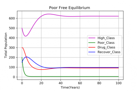
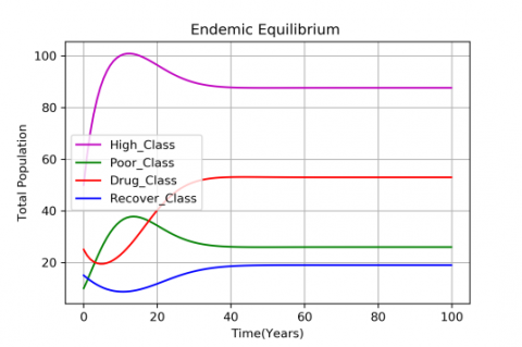
System (1) is simulated for various parameter combinations that fulfill the locally and asymptotically stable (see Figure 3) EE condition E2. We analyze the parameter set S1={μ=0.14, μ1=0.02, α1=0.3, α2=0.7, l1=0.02, l2=0.05, γ=0.07, θ1=0.09, θ2=0.01}, and the parameters are feignted feasible value.
The E1 system (1) has only the PFE shows locally and asymptotically stable [22] (see Figure 2). And also for a different set of parameters in S2={μ=0.12, μ1=0.16, α1=0.65, α2= 0.56, l1=0.02, l2=0.02, γ=0.15, θ1= 0.001, θ2=0.37}.
Figure 2. Plot of poverty free equilibrium (E1)
The system (1) of feasible equilibrium are endemic and poverty free equilibrium has locally asymptotically stable [15] (see Figures 2 and 3) respectively.
Figure 3. Plot of endemic equilibrium (E2)
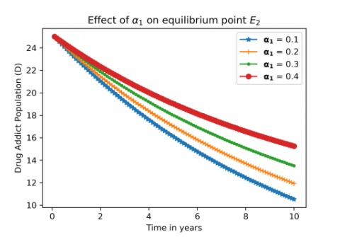
Figure 4. Variation of the compartment drug addiction with the effect of α1
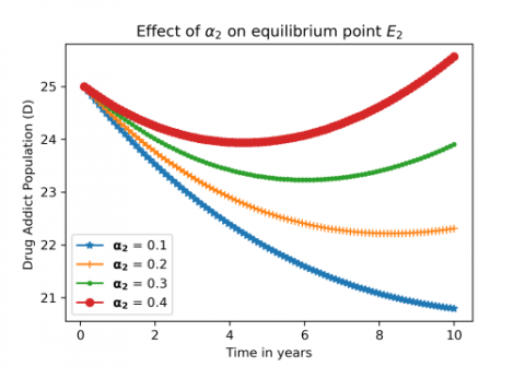
Figure 5. Variation of the compartment Drug Addiction with the effect of α2
Figure 6. Variation of the compartment poor population with the effect of θ1
Figure 7. Variation of the compartment poor population with the effect of θ2 shown in poor people affected pandemic situations
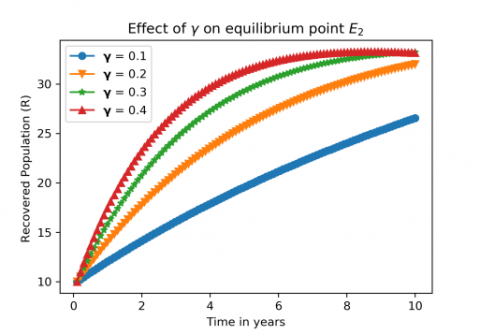
Figure 8. Variation of the compartment recovered population with the effect of γ shown in affected people can recover after the treatment or social media guidance effects
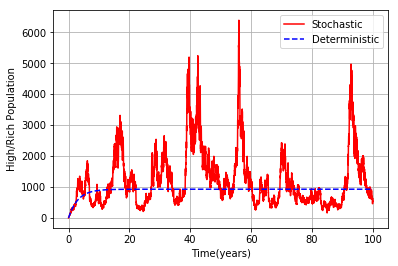
Figure 9. The variation which explores the difference between deterministic and stochastic stability of highclass population
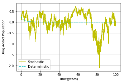
Figure 10. The variation which explores the difference between deterministic and stochastic stability of drug population
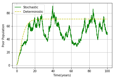
Figure 11. The Variation which explores the difference between deterministic and stochastic stability of poor population
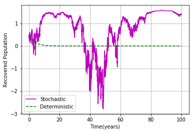
Figure 12. The Variation which explores the difference between deterministic and stochastic stability of recovered population
The Parameters (α1, α2, θ1, θ2, γ) of the system (1) to show the effects of the stability to attain the equilibrium point in different position, (see Figures 4-8) respectively.
The system (1) has different parameters assumed the parameter values are shown the comparisons of deterministic and stochastic model Eqns. (4-7) see Figures 9-12 by numerical simulation [23].
In this section, Adults may be more likely to use drugs if they are lonely or have lost their jobs. Teenagers should avoid moving, family breakups, and changing schools at these times. Indicated programmes are for young people who have already begun to use drugs. The universal program naturally targets risk and protective variables that affect everyone. Awareness and tracking are essential for reducing poverty and its causes. All this is likely if we organize to end suffering to create a wealthy world. We capture efforts to anticipate poverty reduction by utilizing prospective approaches by invoking the mathematical models, and each of them is socially accountable for lowering the persistence of poverty reduction in society.
This model suggested and evaluated to control poverty with this factor in mind. We found the feasibility of the demographic progression from addiction to poverty. Simulations of the system to the fluctuations of the population in various conditions determine the maximum rate of intervention that will alleviate poverty and drug addiction. We will lower the minimum number of members in poverty and drug addiction to the result of this article.
[1] Burnette, C.E., Sanders, S., Butcher, H.K., Rand, J.T. (2014). A toolkit for ethical and culturally sensitive research: An application with indigenous communities. Ethics and Social Welfare, 8(4): 364-382. https://doi.org/10.1080/17496535.2014.885987
[2] Chen, C.A., Wang, P.W., Yen, Y.C., Lin, H.L., Fan, Y.C., Wu, S.M., Chen, C.F. (2019). Fast analysis of ketamine using a colorimetric immunosorbent assay on a paper-based analytical device. Sensors and Actuators B: Chemical, 282: 251-258. https://doi.org/10.1016/j.snb.2018.11.071
[3] Hsu, J., Lin, J.J., Tsay, W.I. (2014). Analysis of drug abuse data reported by medical institutions in Taiwan from 2002 to 2011. Journal of Food and Drug Analysis, 22(2): 169-177. https://doi.org/10.1016/j.jfda.2014.01.019
[4] Mackey, T.K., Liang, B.A. (2013). Improving global health governance to combat counterfeit medicines: A proposal for a UNODC-WHO-Interpol trilateral mechanism. BMC Medicine, 11(1): 1-10. https://doi.org/10.1186/1741-7015-11-233
[5] Oduwole, H.K., Shehu, S.L. (2013). A mathematical model on the dynamics of poverty and prostitution in Nigeria. Mathematical Theory and Modeling, 3(12): 74-80.
[6] Al-Mandhari, A., Hammerich, A., El-Awa, F., Bettcher, D., Mandil, A. (2020). Full implementation of the WHO framework convention on tobacco control in the eastern Mediterranean region is the responsibility of all. Eastern Mediterranean Health Journal, 26(1): 4-5.
[7] Srivastav, A.K., Athithan, S., Ghosh, M. (2020). Modeling and analysis of crime prediction and prevention. Social Network Analysis and Mining, 10(1): 1-21. https://doi.org/10.1007/s13278-020-00637-8
[8] Zhao, H., Feng, Z., Castillo-Chavez, C. (2014). The dynamics of poverty and crime. Journal of Shanghai Normal University (Natural Sciences· Mathematics), 43(5): 486-495. https://doi.org/10.3969/J.ISSN.100-5137.2014.05.005
[9] Sharkey, P., Besbris, M., Friedson, M. (2016). Poverty and crime. The Oxford Handbook of the Social Science of Poverty, 623-636. https://doi.org/10.1093/oxfordhb/9780199914050.013.28
[10] Sharma, S., Samanta, G.P. (2013). Dynamical behaviour of a drinking epidemic model. Journal of Applied Mathematics & Informatics, 31(5_6): 747-767. http://dx.doi.org/10.14317/jami.2013.747
[11] Srivastava, P.K., Banerjee, M., Chandra, P. (2009). Modeling the drug therapy for HIV infection. Journal of Biological Systems, 17(2): 213-223. https://doi.org/10.1142/S0218339009002764
[12] Wilcox, B.A., Echaubard, P., de Garine-Wichatitsky, M., Ramirez, B. (2019). Vector-borne disease and climate change adaptation in African dryland social-ecological systems. Infectious Diseases of Poverty, 8(1): 1-12. https://doi.org/10.1186/s40249-019-0539-3
[13] Sakib, M., Islam, M., Shahrear, P., Habiba, U. (2017). Dynamics of poverty and drug addiction in sylhet, Bangladesh. JMEST, 4(2): 6562-6569. http://www.jmest.org/wp-content/uploads/JMESTN42351992.pdf.
[14] NDDTC, AIIMS submits report “Magnitude of Substance use in India” to M/O Social Justice & Empowerment. https://pib.gov.in/Pressreleaseshare.aspx?PRID=1565001, accessed on Feb. 22, 2022.
[15] Athithan, S., Ghosh, M., Li, X.Z. (2018). Mathematical modeling and optimal control of corruption dynamics. Asian-European Journal of Mathematics, 11(6): 1850090. https://doi.org/10.1142/S1793557118500900
[16] Siva, K., Athithan, S. (2022). Analysis of solution for the stochastic model representing water scarcity in the society. Mathematical Modelling of Engineering Problems, 9(4): 1031-1042. https://doi.org/10.18280/mmep.090421
[17] Chinnadurai, K., Athithan, S. (2022). Mathematical modelling of unemployment as the effect of COVID-19 pandemic in middle-income countries. The European Physical Journal Special Topics, 231(18-20): 3489-3496. https://doi.org/10.1140/epjs/s11734-022-00620-8
[18] Yuan, Y., Allen, L.J. (2011). Stochastic models for virus and immune system dynamics. Mathematical Biosciences, 234(2): 84-94. https://doi.org/10.1016/j.mbs.2011.08.007
[19] Rajalakshmi, M., Ghosh, M. (2018). Modeling treatment of cancer using virotherapy with generalized logistic growth of tumor cells. Stochastic Analysis and Applications, 36(6): 1068-1086. https://doi.org/10.1080/07362994.2018.1535319
[20] Stella, I.R., Ghosh, M. (2019). Modeling plant disease with biological control of insect pests. Stochastic Analysis and Applications, 37(6): 1133-1154. https://doi.org/10.1080/07362994.2019.1646139
[21] Srivastav, A.K., Ghosh, M., Chandra, P. (2019). Modeling dynamics of the spread of crime in a society. Stochastic Analysis and Applications, 37(6): 991-1011. https://doi.org/10.1080/07362994.2019.1636658
[22] Chinnadurai, K., Athithan, S. (2020). Mathematical modelling of poverty dynamics with the effect of alcohol consumption. In AIP Conference Proceedings, 2277(1): 130001. https://doi.org/10.1063/5.0025263
[23] Ferreira‐Borges, C., Rehm, J., Dias, S., Babor, T., Parry, C.D. (2016). The impact of alcohol consumption on African people in 2012: An analysis of burden of disease. Tropical Medicine & International Health, 21(1): 52-60. https://doi.org/10.1111/tmi.12618