Basim M. Al-Zaidi*![]() | Jamal S. Makki
| Jamal S. Makki![]() | Mohammad H. Al-Umar
| Mohammad H. Al-Umar![]() | Abaas J. Ismaeel
| Abaas J. Ismaeel![]()
© 2023 IIETA. This article is published by IIETA and is licensed under the CC BY 4.0 license (http://creativecommons.org/licenses/by/4.0/).
OPEN ACCESS
The study consists of building a hydraulic model that can account for the effect of the slope of the pipeline on the pumping system performance. The model system is about a single perforated pipe with several different sizes opening holes equally distributed along the pipe and connected to the pump at the inlet, while the other end of the pipe is closed. The model was applied and implemented in several cases of pipe slope level, uphill, and downhill. Results have been shown for the case of equilibrium between the pump and the pipe system that the pressure head at the beginning of the pipe will increase when is in an uphill slope but inflow decreases because of the deficit in the pressure head and flowrate at the middle and end of the pipe and vice versa. A reasonable agreement between the model and previous studies was achieved for the model validation and accuracy. Also, the study showed that there is a large change in pressure head and flowrate along the pipe due to the change in elevation along the modeled pipe. The capacity of the system decreases in the case of an uphill slope and becomes lesser than the design capacity and decreases with increasing the slope value. More power is needed to adjust the differences between the actual and calculated system curve, and in sequences increase the cost of the pumping and decrease the efficiency of the pump. While in the case of a downhill slope, the capacity of the system is higher than the design capacity. In turn, less power is required to adjust the design operation point and low cost of the pumping, but there is a slight decrease in the efficiency of the pump. Also, the study concluded that the slope of the pipeline is a key issue in the design of the pumping pipeline system to reduce energy consumption and cost. This study can be considered a useful tool to perform the pumping system under various conditions of the hydraulic system.
pump, performance, pipeline, slope, efficiency, cost
The pumping of water is considered one of the earliest use of machines in human life to construct the earliest civilization. The machine of pumping has evolved and taken several shapes from the waterwheel to what is known today as pumps. Today, pumps are the most widely used machines [1]. One of the most important engineering applications of hydraulics principles is the design and operation of fluid machinery such as pumps [1, 2]. Pumps are hydraulic machines designed to convert mechanical energy to hydraulic energy. The purpose of this machine is to transfer the mechanical energy of a rotating shaft to fluid energy in the form of an increased pressure head [3]. Centrifugal pumps are the most widely used type, in a centrifugal pump, an impeller turns at a high rotational speed, supplying kinetic energy to the liquid entering the center of the impeller [4]. The centrifugal force created by the rotating impeller moves the liquid out along the impeller blades, increasing kinetic energy. After the fluid leaves the impellers, it exits the pump through a spiral casing of increasing cross-sectional area (the convolute), at which time, the kinetic energy is converted to work energy, i.e., pressure head [5]. The integral two parts of many pumping systems are the pump and pipeline [4, 6, 7] which are connected by the fluid. The fluid moves in the system based on the change in pressure [8]. The pressure head in the piping system is necessary to maintain the flow of the fluid in the system. Pumps are considered the source of pressure in the pipeline system due to their energy consumption [4].
Many studies have been concerned about the performance of the pumps under various conditions of the pumping pipeline system and the problem is still under consideration. Jani et al. [9] studied the factors that impact the performance of the pumping system using an evaluated network model. The study stated that the performance of the pumping system mainly depends on several important factors, the first sufficient parameter to be considered is pump efficiency, and the other crucial factors involve the contribution of pipes in resistance to flow due to size and pressure drop. Counting these factors together in the studied system can help for saving energy in the system. The study concluded that to understand the overall impact on the performance of a pumping system it is essential to study the feasibility of such measures that can optimize the data and improve the performance of the network based on a municipal water distribution system. Rafael et al. [10] presented a study to examine the pipeline behavior before putting the system into operation. The case study is an existing water pipeline system consisting of five pumping stations each station is equipped with five pumps. The system is about a 90 km pipeline with a total head difference is 326 m. The study stated that protecting the line against low pressures, which is considered an attempting unconventional form, is of necessity to start supplying water to the population. The study suggested that operate two of five units per plant and allowing air to enter the system through the valves located along the pipeline. The air entrained formed stationary pockets at high points of the pipeline. In consequence, these pockets absorbed the energy of transient pressure waves through the system. Furthermore, due to the limited inertia of the motors, the speed of the pump will rapidly decrease and this let to generate low-pressure waves and inconsequence to create water column separation [11, 12]. Aissa [13] presented a study to determine the effects of changes in the inlet conditions of a pumping system. The study investigated the performance of a baseline centrifugal pump both analytically and experimentally by comparing the main characteristics of the baseline without obstacle pump and those of the pump with obstacle. The study involved both the normal suction condition of the centrifugal pump (baseline configuration) and the condition at which an interfering plate is mounted in the pump intake, distorting the flow at the pump suction. The study concluded that the performance of centrifugal pumps at both design and specific off-design speeds is significantly affected when the interfering plates; straight or inclined, are mounted at the suction side. Thus, mechanical power the overall efficiency is greatly affected. Dhaiban [14] provided an experimental study to determine the effect of changing the inlet diameter and inlet water level to the head and the amount of flow rate at the exit of a pumping system. Also, the efficiency of the tested system was evaluated. The study results showed an inverse relationship between the head and the amount of flowrate at the outlet where the head and flowrate at the exit are not affected by pressure changing inside the vessel. The study showed that the maximum efficiency depended on the potential energy of water and reach about 29% at the supply tank height of 1.9 m and inlet diameter of 0.5 in. The maximum enhancement reached 17% when compared with other studies at the same supply head of 1.8 m.
The total head that a pump develops for a given flowrate depends on the elevation change and friction and minor losses [15]. The elevation difference (the interpretation is that a pump is being used to move water to a high level) is termed static lift [4]. The friction loss and minor losses depend on the water velocity in the pipe, thereby varying directly with the flowrate, and are known as the dynamic lift terms [16]. The sum of the static and dynamic lift terms is known as the total dynamic head. The primary purpose of a pump is to add energy (pressure head) to the fluid system to compensate for the head loss incurred by friction and appurtenant fittings in all types, and/or to raise the water to a higher elevation. Pumping needs energy and thus the wrong selection of the pump may result in higher costs and poor performance of the system [17]. Therefore, it is essential to choose the correct pump that fits the system requirements. In comparison with other types of pumps, Centrifugal pumps are quite common due to their high efficiency, flexibility in operation with variable heads, and continuous flowrate [4]. The characteristic curves present the performance of a centrifugal pump, and these curves are comprised of several terms, which usually are pumping head versus flowrate, input power against flowrate, and efficiency against flowrate [17]. If the performance curves of the pump are not given by the manufacturers, and to produce such operation curves, the test of the pump should be done first in the laboratory under various conditions of head and discharge before putting the pump into operation [1, 18]. In the pumping pipeline system, the criteria for the selection of pumps is mainly based on what best serves the requirements reasonably well of the project such as the efficiency and pumping cost [19, 20]. Starikov [21] provided a study aimed to minimize energy consumption by providing control of oil pumping through the pipeline with recommendations for using Plant Wide Control (PWC) technology. The study stated that the proposed engineering method of using pipeline management (PWC) can minimize the energy loss of power at the expense of the balance of the operation of pumping stations that take place on the pipeline. The study concluded that PWC method allowed control of the operating points of the pump unit and provided maximum throughput opportunity with a reduction of consumed energy. Stefano et al. [22] presented such a study aimed to minimize the costs of energy by maximizing pumping during periods of off-peak electricity tariff. The study presented a method for controlling a pumping plant with a tank as a water supply. The results showed that this method can lower the energy cost as compared with that obtained using fixed trigger levels. Moreover, the proposed methodology was more suitable when compared with those resulting from using the scheduling of the pump in which several pumps are switched together. Further, unlike scheduling of the pump, using the proposed method does not need forecasting of water supply and frequent best scheduling, thus it gives a sufficient tool for pumping plant operation. Therefore, representing an adequate methodology for pumping pipeline operation systems is essential in fluid studies.
The scope of the present study is to account for the effect of the pipeline slope on the pump performance, pump efficiency, and cost of pumping, where factors such as pressure and head loss usually dominate the pumping system. This can be achieved by considering the effect of pipeline slope on pump performance to provide additional useful information when operating the hydraulic system. The objective herein is to apply the fluid hydraulic principle to predict the change of pressure due to the change in pipe slope and the consequence to predict what is the impact of this condition on the performance, cost, and efficiency of the pumping system.
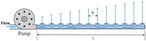
The model consists of two integrated parts pump and a pipeline. The length of the modeled pipe is assumed to be 400 m, and the pipe is perforated with 10 opening holes equally distributed along the pipe, i.e., 10 m reach. The position of the first hole lies at a distance of 10 m from the inlet of the pipe, i.e., at the end of the first reach. The other end of the pipe is closed, thus the pressure near the closed end of the pipe is high, and there will be high flow through the holes (nozzles) near the end. Therefore, we have to vary the size of the holes along the perforated pipe and then the discharge (see Figure 1). The modeling procedure is simulated in two stages:
The network pipe, in general, is usually designed based on zero slopes (horizontal), i.e., the pipe is level and then accounting for the effect of the slope on the design by analyzing the change in elevation in each slope. In this stage of the modeling, we compute the following:
i. Compute the nozzles discharge along the modeled pipe
Figure 1. Schematic of the pumping pipeline system
The discharge of any nozzle along the pipe starting from the start point is proportional to the total discharge, i.e., the pump discharge.
$\mathrm{q}_{\mathrm{nzl} \mathrm{n}}=\frac{2 \mathrm{n} \mathrm{R}^2}{\mathrm{~L}^2} \mathrm{Q}_{\mathrm{t}}$ (1)
where, qnzl is the discharge of the nozzle (hole) (m3/hr), Qt is the total discharge (m3/hr), L is pipe length (m), and R is the reach length between two holes (m), and n is the number of the hole.
ii. Calculate head loss due to friction
The major losses in pipe flow are the losses caused by established pipe friction. These losses in energy are based on several factors such as the type of pipe, i.e., the roughness of the inner surface of the pipe, pipe diameter, length of the pipe, fluid properties, and pipe discharge. There are several formulas to determine the losses in pipes. One of these formulas is Hazen-Williams [23].
$\mathrm{H}_{\mathrm{f}}=1.14 \times 10^9\left(\frac{\mathrm{Q}}{\mathrm{C}}\right)^{1.852}\left(\frac{\mathrm{L}}{\mathrm{D}^{4.87}}\right)$ (2)
where, Hf is head losses due to friction (m), Q is pipe discharge (m3/s), D is the inner diameter of the pipe (mm), and C is the roughness coefficient of the pipe (C=130). The roughness coefficient of the pipe depends on relevant factors such as the type of pipe material, suspension, and the age of the used pipe. The study assumed a known roughness coefficient considering experimental data of real pipelines from the previous studies declared by the pipe manufacturer as input to the model. The head loss in pipes due to friction depends on the friction factor whereas the friction factor depends on the Reynolds number and relative roughness of the pipe.
The determination of the head losses due to friction for the whole pipe using Eq. (2) needs to compute the value of the head losses for each segment with the length (R) of the perforated pipe between the holes. The head of the nozzle at the end of the pipe and knowing that the head at the inlet of the pipe is computing using the following equation:
$\mathrm{H}_{\text {new }}=\mathrm{H}_{\mathrm{old}}-\mathrm{H}_{\mathrm{f}} \pm \Delta \mathrm{z}$ (3)
where, Hnew is the pressure head of the nozzle of the new elevation (m), Hold is the pressure head of the nozzle in the case of horizontal pipe (m), and Δz is the difference in elevation between the ends of the pipe determined by the slope and pipe length. The sign of the last term in Eq. (3) is positive when the slope of the pipe is down and negative with slope is up. Eq. (3) is used to determine the pressure head at any nozzle along the modeled pipe. The change in elevation along the pipe affects the nozzle pressure head and in consequence the nozzle discharge. Thus, Eq. (1) can be modified to compute the new discharge of the nozzle for the new elevation as follows:
$q_{\text {new }}=q_{\text {old }} \times \sqrt{\frac{\mathrm{H}_{\text {new }}}{\mathrm{H}_{\text {old }}}}$ (4)
where, qnew is nozzle discharge in the case of elevation change (m3/hr), and qold is nozzle discharge in the case of horizontal pipe (m3/hr).
iii. Compute the discharge along the molded pipe
Based on the continuity equation, the discharge along the pipe decreases in the flow direction. The discharge of the first segment of the pipe is equal to the total discharge and then it decreases after each hole along the pipe by subtracting the hole discharge from the total discharge using the following equation.
$\mathrm{Q}_{\mathrm{i}}=\mathrm{Q}_{\mathrm{t}}\left[1-\frac{\mathrm{L}^2}{\mathrm{R}^2} \times \mathrm{i} \times(\mathrm{i}-1)\right]$ (5)
where, Qi is the discharge passing in the reach i of the pipe (m3/hr).
The change in the slope of the pipe impacts the pressure head and discharge along the modeled pipe and thus the input discharge and the input head will affect it, and this is not isolated from the pump performance, so it leads to a balance point between the pipe system and pump. The main objective here is to find this point on the pump characteristic curve to make an equilibrium case with the input discharge and the pressure head at the inlet. The movement of the equilibrium point from one position to another along the curve will influence pump efficiency and then the pump cost because the cost increases with decreased efficiency.
$P R C=B P \times Y H \times U P C$ (6)
where, PRC is the required cost of pumping, YH is the annual working hours of pumping, UPC is the cost of electricity, and BP is the power per unit pumping (kW). The power per unit pumping (BP) in kW computed from the following equation:
$\mathrm{BP}=\frac{\mathrm{Q}_{\mathrm{p}} \times \mathrm{TDH}}{367 \times \mathrm{EP}}$ (7)
where, Qp is pump discharge (m3/s), TDH is the total dynamic head of pumping (m), and Ep is the total efficiency for unit pumping (Pump efficiency X Shaft efficiency).
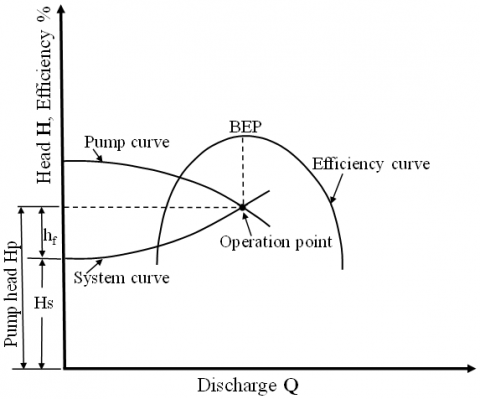
The questions here are what are flowrates should we use? Where do the system head curve and the pump performance curve intersect? The answer to this question is we have to use flowrates listed in the pump performance curve which represents the illustration of pump performance and system curves as shown in Figure 2. The selection of the pump is based on several steps such as determining the design flow, developing the system head curve, checking the agreement of the design flow, operating point (s), and best efficiency point (see Figure 2). The pump performance curve represents also the energy usage by the pump. The power to operate the pump is directly proportional to the discharge head, and fluid density, and is inversely proportional to the efficiency of the pump. It is desirable to select a pump that operates close to the peak of the efficiency curve or at the best efficiency point (BEP). It is best to choose the pump that will operate at the highest efficiency. The pumps that operate at close to their efficiency have long life [3]. Centrifugal pump is most used for water and wastewater pumping. The head is developed principally by centrifugal force. The discharge is related to the specific speed and the pressure conditions under which the pump operates. Searching the pump manufacture catalogs for a single centrifugal pump that will produce m of the head at gpm, i.e., from the pump characteristics diagram at the required gpm the pump will generate m of the head, and thus it will fit the requirements reasonably well.
Figure 2. Illustration of pump performance and system curves
The system curve is developed from the application of the energy equation between intake and delivery points and accounts for the head provided by the pump and various minor and major losses. The point at which the system curve intersects the performance curve is termed the operating point. Usually, 3 points are required to define a pump curve, typical points are the shutoff head, the most efficient point, and the maximum flow. While the best-fit curve can also be determined when more than three points are specified. The system head is the net of the work on a unit of fluid by the pump and is given by the following equation:
$H_s=S L+D L+D D+h_m+h_f+h_o+h_v$ (8)
where, Hs is the system head, SL is the suction-side lift, DD is the drawdown of source water, hm is the minor losses, hf is the major losses, i.e., losses due to friction, ho is the operating pressure head, and hv is velocity head (V2/2g). Suction and discharge static lifts are measured when the system is not operating, DD, drawdown, is the decline of the water surface elevation of the source water due to pumping (mainly for wells), DD, hm, hf, ho, and hv all increase with increasing pumping capacity Q.
The efficiency of the pump is usually determined by brake horsepower (BHP) as follows:
BHP = power that must be applied to the shaft of the pump by a motor to turn the impeller and impart power to the water:
$E p=\frac{\text { output }}{\text { input }}=\frac{\text { WHP }}{\text { BHP }} \times 100$ (9)
Ep never reaches 100% due to energy losses due to many reasons such as friction in bearings around the shaft, moving water against pump housing, etc. the Centrifugal pump efficiencies range from 25 to 85%. If the pump is incorrectly sized, this means Ep is lower. Some of the characteristic pump curves are head decreases as capacity increases. The efficiency of the pump increases when capacity increases to a certain point, and BHP increases as capacity increases to a certain point where:
$\mathrm{BHP}=\frac{100 \times \mathrm{Q} \times \mathrm{HS}}{3960 \times \mathrm{Ep}}$ (10)
The power cost for the pumping in pressurized pipes depends on several factors such as pump flowrate, total dynamic head, the efficiency of the pump and motor, the number of operating hours per year, and the cost of the energy unit. The movement of the equilibrium point from one position to another along the system curve affects the pump efficiency, where pumps are always operating at this point with high efficiency, and pumping cost increases with decreased efficiency. The movement of the balance point means a change in flow and head of the system to get the equilibrium, and thus the pump delivers an amount of water different from the required in the system. Knowing the power per unit pumping, the annual working hours of pumping, and the cost of electricity, the required cost of pumping can be estimated (Eq. (6)).
The best efficiency point coincides with the required operation point, the curve of the efficiency is concave downward (see Figure 2) and the power is increasing curve. If a lower operating flow and the same power are delivered, the pump acts as a turbine. If a higher discharge is delivered, the pump is required more power, but the pump efficiency would decrease and hence the energy would not be optimal. The line passing through these points could be around, near, or coincide with the line passing the operation point and best efficiency point (BEP). The determination of these points is, one lies on the system curve, the second on the efficiency curve, and the third one is the value of BHP that is computed from Eq. (10).
The model is written in Python code, and the spatial intervals used in the simulations can be varied between 0.5 m and 50 m.
The model is run for different cases of pipe slope uphill, level, and downhill. The results of the model can be presented in three stages as follows:
In this stage, we compute the input flowrate and the pressure head at the begging of the modeled pipe for different values of the assumed pressure head at the end of the modeled pipe.
i. Level pipe (zero slope)
Pipes, in general, are designed based on the energy head and head losses, thus the slope of the pipe is not taken into consideration in the design criteria. First, we study the case when the pipe is level, i.e., zero slope, and then we study the effect of the slope on the modeled pipe. The discharge of the nozzles along the pipe is computed using Eq. (1), which is the case when the pipe system is designed. The input discharge is 324 m3/hr and the pressure head at the begging of the pipe is 58.5 m.
ii. The slope of the pipe upward (+ve slope)
The change in elevation of the nozzles along the modeled pipe resulted in a change in pressure and flowrate in these nozzles. When the pipe slopes upward, the pressure inside the pipe decreases, and in consequence, the pressure of the nozzles also decreases. This will influence the flowrate of the nozzles along the pipe and the pressure head at each nozzle and this as result impacts the total input discharge and the total head at the begging of the pipe. The method of accounting for the impact of slope on nozzles can be represented by nozzle discharge which depends on the change in the head (h) that resulted from the change in slope by using the orifice equation as follows:
$\mathrm{q}=C_d \mathrm{a} \sqrt{2 \mathrm{gh}}$ (11)
where, q is nozzle discharge (m3/hr), a is the area of the cross-section of the nozzle (free jet) (m2), h is the pressure head at the nozzle (m), Cd is orifice coefficient (0.95-0.98), and g is the acceleration of gravity (m/s2).
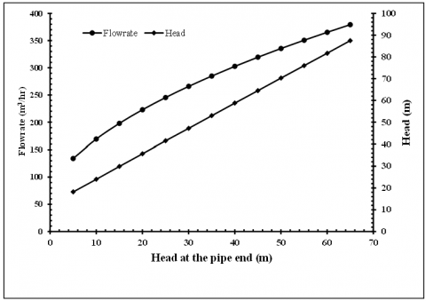
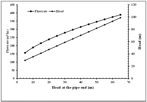
Figures 3, 4, and 5 show input discharge and pressure head at the begging of the pipe for the different assumed values of the pressure head at the pipe end in the case of the upward slope. We can see from these results that the value of the discharge at the begging of the pipe and pressure head at the begging of the pipe decrease with decreasing the head at the end of the pipe.
Figure 3. The input discharge and pressure head at begging of the pipe for the different assumed values of the head at the pipe end in the case of the upward slope of 3%
iii. The slope of the pipe downward (-ve slope)
In this case, the slope of the pipe is downward, the pressure inside the pipe increases along the modeled pipe, and then the pressure head at the nozzles, in this case, is higher than that value in the case of a level pipe. The increase in the pressure head increased the discharge of the nozzles along the pipe. With the elevation difference being high as a comparison with the level case, the increase in pressure will be high, and increasing in the nozzles discharge will be large. It is noticed that from these results the increase in discharge of the nozzles at the end of the pipe is higher than the increase in the discharge of the nozzles at the beginning of the modeled pipe. This is due to the large change in the elevation at the end of the pipe. This increase in the discharge of the nozzles influences the input discharge at the begging of the pipe and the head at the beginning of the modeled pipe.
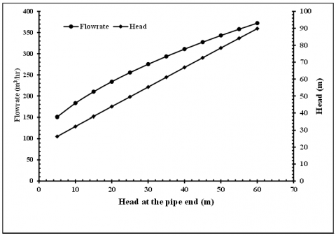
Figure 4. The input discharge and pressure head at begging of the pipe for the different assumed values of the head at the pipe end in the case of the upward slope of 5%
Figure 5. The input discharge and pressure head at begging of the pipe for the different assumed values of the head at the pipe end in the case of the upward slope of 6%
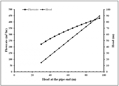
Figures 6, 7, and 8 present the values of the input discharge and pressure head at begging of the pipe for the different assumed values of the pressure head at the end of the pipe in the case of a downward slope (-ve slope). It is clear from the results of these model runs, that the discharge and pressure head at the begging of the pipe increase with increasing the pipe slope and the increase in the pressure head at the end of the pipe for one slope.
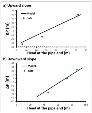
For purpose of model validation and accuracy, the model results were compared with the available data provided by a previous study [24], which presented similar cases to the modeled cases in this study. Figure 9 shows a comparison between the model results with the available data for the difference in pressure head. The black line represents the model results and the blue dots are the limited available data, Δp is the pressure difference at the begging of the pipe between the case of slope (upward or downward) and the case of horizontal. Reasonable agreements with the limited available data were achieved. The errors in the catching of the data are due to the limited available data of slopes. The available slopes in this comparison for the upward and downward cases are only 5.8% which are ~ close to the studied cases of the slope in this study (i.e., 6%).
Figure 6. The input discharge and pressure head at begging of the pipe for the different assumed values of the head at the pipe end in the case of a downward slope of 3%
Figure 7. The input discharge and pressure head at begging of the pipe for the different assumed values of the head at the pipe end in the case of a downward slope of 5%
Figure 8. The input discharge and pressure head at begging of the pipe for the different assumed values of the head at the pipe end of the pipe in the case of a downward slope of 6%
Figure 9. Comparison between model results and the available data
This stage deals with the case of system equilibrium, i.e., the equilibrium between the pump and the system. The pump used in the system works on a curve called the pump performance curve as shown in Figures 2, and 10, and the head curve of the system shows the head requirement to generate the required range of flowrates. The objective here is to determine the case of the equilibrium, i.e., equilibrium between the pump and input discharge of the pipe and pressure head at begging of the modeled pipe for all studied cases of the slope. After getting on the values of the input discharge and the pressure head for all the studied cases, we can get to the points of equilibrium with the pump curve and for all the cases by drawing the values of the input discharge with the pressure head and for all the cases and draw the pump curve and find the points of intersection, i.e., the points of equilibrium for the system and pump performance characteristics.
The pump operation point is the point of intersection between the pump performance curve (H) and the system head curve (Ep). Given a simple pipe system with a pump to lift water from a well into a pipe. The well is assumed at an elevation of 0 m and the water level at the start point is at an elevation of 12 m. The connecting pipe is 400 m of 8 in CIP with CHW = 100. A check valve, gate valve, bends, etc., result in a minor loss coefficient km = 4.0 (hm = km Q2). The question here is what the flowrate is if the pump has the following performance curve. The solution to this problem involves determining the pump operation point, i.e., the intersection of the performance curve of the pump and the head curve of the system, by evaluating the modified Bernoulli equation for a range of flow; use the flows given for the pump performance curve. Then plot the pump performance and system head curve (SHC). The system curve represents the performance curve of the piping system. This illustrates the use of exhaustive search to progressively locate the point where the performance curve of the pump (H) and the head curve of the system (Ep) intersect. This intersection determines both the pump head and flowrate.
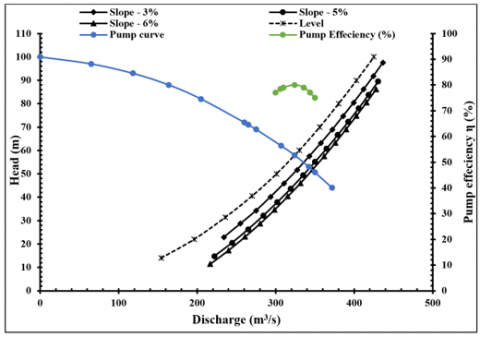
Figure 10 presents the evaluation of pump performance with the system with a slope upward. Where the dashed line is the system when the slope is zero. Figure 10 clearly shows the intersection between the performance curve of the pump and the system curves, the actual curve (the dashed line, i.e., zero slope), and the calculated curves (the curves of the upward slopes). The operation point of the pipeline may affect the required capacity of the pump, the total head in the pipeline, and then the operation point in the discharge-head coordinates (Q, H). The expected operation capacity of the pump and system is 324 m3/s (i.e., the design capacity), but the delivered capacity is less than the design capacity. The discharge pressure is higher than calculated, the speed is high, and hence the pump is using too much power. Thus, more power is required to adjust the differences between the actual and calculated system curves.
Figure 10. Evaluation of pump performance with the pumping system for the case of the upward slope
Figure 11. Evaluation of pump performance with the pumping system for the case of the downward slope
Figure 11 presents the evaluation of pump performance with the system with a slope upward. Where the dashed line is the system when the slope is zero. The expected operation capacity of the pump and system is 324 m3/s (i.e., the design capacity) but in this case, downward slopes will deliver capacity higher than the design capacity. In some systems, control valves may be suggested to install in the discharge line to adjust for these variations between the calculated and actual system curves.
Figures 10 and 11 represent the performance curve of the pump plotted together with the system curves, the objective herein is to show the change in flowrate resulting from a change in the total head of the system in all studied cases. It seems the magnitude of the change in flowrate depends on the pattern of the system curve and the increasing amount in the pressure head. From the results shown in Figures 10 and 11, the points of equilibrium for the system curve with pump performance curve for both cases of slope upward and downward and pump efficiency for each case. The curves intersect at a particular flowrate, i.e., the operation point. This point represents the maximum flowrate the pump can deliver to the system and hence the maximum capacity of the pump. For the amounts of flowrates below this value in the operation point, the pump delivers a higher head than the required value and the amounts of flowrates above this value result in a pump head less than the required system head. Therefore, for any particular piping system, the operation point of the centrifugal pump is only the point where the curves intersect. The problem is associated with pumping in the case of the operating capacity being greater than the design capacity. The increase in the amount of the flowrate will result in the pump using power more than expected, and in consequence which may overload the motor to allow for the safe operation of the system at capacities slightly higher than the design flow. The cycle repeats when the pump again has the old cases of the head in the system. The head losses increase due to an increase in friction losses with the liquid velocity that passes through the system. We can conclude from the model results that the pump efficiency is high when the slope is close to the level case and the efficiency decreases with increasing the value of the slope. Table 1 summarizes the points of equilibrium for the system and pump performance for all the cases of the slope with pump efficiency. We can get on the pressure head at the end point of the pipe using the points of equilibrium presented in Table 1 by using interpolation or using the same program code but by assuming the values of the pressure head at the pipe end to get on the flowrate and pressure head at begging of the pipe at the equilibrium case.
Table 1. The points of equilibrium for the system and pump performance for all the cases of the slope with pump efficiency
|
Slope (%) |
Upward |
Level |
Downward |
||||
|
6% |
5% |
3% |
0% |
-3% |
-5% |
-6% |
|
|
Q (m3/hr) |
300 |
306 |
310 |
324 |
336 |
344 |
350 |
|
Head (m) |
65 |
64 |
61 |
58 |
55 |
53 |
51 |
|
η (%) |
77% |
78% |
79% |
80% |
79% |
76% |
75% |
Table 2. The pressure head at the end of the pipe for all the cases of the slope
|
Slope (%) |
Upward |
Level |
Downward |
||||
|
6% |
5% |
3% |
0% |
-3% |
-5% |
-6% |
|
|
Head (m) |
35.6 |
37.5 |
41.9 |
50 |
57.8 |
63.15 |
64.2 |
Table 2 represents the pressure head at the end of the modeled pipe for all the studied cases of the slope. The pressure head at the pipe end for each case of the slope is used to compute the discharge of the nozzles along the modeled pipe, which represent the case of equilibrium.
From the results of the model runs we can conclude that the capacity increase when the slope of the pipe is down. The friction head losses increase with the increasing capacity while the piezometric heads of the system fairly stay constant and are not changing with the capacity. The best efficiency point (BEP) is changed based on the pump operation point and moves with system work. The BEP is when the system gives high efficiency with the pump operating point. The speed of the pump changed with changing the slope of the modeled pipe. Where the pump is using too much power if the speed is too high. The viscosity of the liquid may become higher than the expected liquid viscosity. The discharge pressure is higher than the calculated. Even a small change in the head of the system can create significant changes to the flowrate. Where a 6% decrease in the downward pipe slope causes a 12% reduction in head and an almost 8% increase in flowrate. While a 6 % increase in the upward pipe slope causes a 12.4% increase in head and an almost 7% reduction in flowrate. The discharge varies linearly with an increase in pump speed and the power with an increase in impeller diameter. Similar relationships can be developed for pump head and power. When the speed increases the pump head increase, power increases, and then efficiency decreases. The efficiency of a pump depends on its discharge, head, and power requirements. Pumps are always operating at the intersection point where the system curve intersects with the performance curve of the pump with high efficiency. The pumps that operate at close to their efficiency have long life [3]. In the case of a change in the system head during normal operation, it is essential to represent system curves for the expected range of high and low levels and then determine if the selected pump will deliver flows at a suitable range. Changing the position of the operating point of the pump is due to the differential pressures at the head of the pump caused by the change in the elevation of pipes. The results show that the increase in the upward pipe slope by 6% cases 8% increased the power by about 10% and the cost of the pumping increased by 7.8%, while the reduction in the downward pipe slope cases by 2% increased in the power and the increase in the cost of the pumping by about 2%. The model results give a reasonable agreement with the observations that were provided by a previous study [9] about evaluation network systems, where pressure head, flowrate, consumed power, efficiency, and cost were indicated for a hydraulic system of networks of pipes and pump stations. Therefore, more power is required in the case of an uphill slope, while less power is needed in the case of a downhill slope. The pump provides a waste of energy to the water by increasing the losses in the pipeline and the situation must be dealt with to improve the performance of the pumping pipeline systems.
In this study, we built and implemented a hydraulic model that is able to account for the effect of the pipe slope on the pump performance and we applied the model to different cases of pipe slope. Three different cases of pipe slope have been studied level, upward, and downward. The pertinent conclusions reached in this study are the pump capacity decreases when the pipe slope is upward and increases when the pipe slope is downward this is when the pipe slope is upward causing a high-pressure head downstream. The efficiency of the pump decreases with increasing the slope of the pipe system. The capacity of the pump decreases with increasing the upward slope and led to increasing the cost of the pumping. While the capacity of the pump increase in the case of the downward slope and increases with the increasing slope of the pipe while the cost of the pump slightly increases in this case. Also, we can conclude that the gradient of the pipeline is a key issue in the design of the pumping pipeline system to reduce energy consumption and cost. The present study helps to simulate and develop the proposed pumping pipeline and analyze the condition properly for any hydraulic system, and then this will give a clear understanding of the overall performance of the pumping pipeline system.
|
a |
cross-sectional area of the nozzle, m2 |
|
BHP |
brake horse power of the pump, kW |
|
BP |
power per unit pumping, kW |
|
C |
roughness coefficient of the pipe |
|
Cd |
orifice coefficient |
|
D |
Pipe diameter, mm |
|
DD |
water source drawdown |
|
Ep |
total efficiency of unit pumping, % |
|
g |
acceleration due to gravity, m.s-2 |
|
h |
head at the nozzle, m |
|
Hf |
head losses due to friction, m |
|
hm |
minor losses, m |
|
Hnew |
pressure head at the nozzle of the new elevation, m |
|
ho |
operating head pressure, m |
|
Hold |
pressure head at the nozzle in the case of the horizontal pipe, m |
|
hv |
velocity head, m |
|
Hs |
system head, m |
|
L |
length of the pipe, m |
|
n |
Number of holes |
|
PRC |
required pumping cost |
|
q |
nozzle discharge, m3/s |
|
Q |
pipe discharge, m3/hr |
|
Qi |
discharge passing in the reach I, m3/hr |
|
qnew |
new nozzle discharge, m3/hr |
|
qnzl |
nozzle discharge, m3/hr |
|
qold |
nozzle discharge in the case of the horizontal pipe, m3/hr |
|
Qp |
pump discharge, m3/hr |
|
R |
reach between two holes, m |
|
SL |
section side left |
|
TDH |
total dynamic head of pumping, m |
|
UPC |
cost of electricity, % |
|
v |
the velocity of the flow, m/s |
|
YH |
annual working hours for pumping, hr |
|
Greek symbols |
|
|
Δp |
the pressure difference at the begging of the pipe between the case of slope and the case of horizontal, m |
|
Δz |
the difference in elevation between the ends of the pipe, m |
|
Subscripts |
|
|
new |
new elevation |
|
old |
old elevation |
[1] Energy, U.D.O. (2006). Energy efficiency and renewable energy. Improving Pumping System Performance–A Sourcebook for Industry, 122.
[2] Volk, M. (2013). Pump Characteristics and Applications. CRC Press. Third edition. Taylor & Francis Group, LLC.
[3] Kothandaraman, C.P., Rudramoorthy, R. (2007). Fluid Mechanics and Machinery. New Age International (P) Ltd., Publishers.
[4] Dhaimat, O.H., Al-Helou, B.A. (2004). The role of centrifugal pumps in water supply. Journal of Applied Sciences, 4(3): 406-410. https://doi.org/10.3923/jas.2004.406.410
[5] Li, Q.Q., Li, S.Y., Wu, P., Huang, B., Wu, D.Z. (2021). Investigation on reduction of pressure fluctuation for a double-suction centrifugal pump. Chinese Journal of Mechanical Engineering, 34: 12. https://doi.org/10.1186/s10033-020-00505-8
[6] Benedict, R.P. (1980). Fundamentals of Pipe Flow. John Wiiley and Sons, Inc., New York, USA.
[7] Hwang, N.H., Houghtalen, R.J., Akan, A.O., Hwang, N.H. (1996). Fundamentals of hydraulic engineering systems (No. TC160. H8213 1981.). Upper Saddle River, NJ: Prentice Hall.
[8] Shim, H.S., Kim, K.Y. (2020). Relationship between flow instability and performance of a centrifugal pump with a volute. ASME Journal of Fluids Engineering. 142(11): 111208. https://doi.org/10.1115/1.4047805
[9] Jani, M., Manure, S., Dave, M.G. (2017). Hydraulic network modeling and optimization of pumping system. International Journal Advanced Research, 5(4): 1035-1046. http://dx.doi.org/10.21474/IJAR01/3912
[10] Carmona-Paredes, R.B., Pozos-Estrada, O., Carmona-Paredes, L.G., Sánchez-Huerta, A., Rodal-Canales, E.A., Carmona-Paredes, G.J. (2019). Protecting a pumping pipeline system from low-pressure transients by using air pockets: A case study. Water, 11(9): 1786. http://doi.org/10.3390/w11091786
[11] Chaudhry, M.H. (2014). Applied Hydraulic Transients, 3rd ed. Springer, New York, USA, 2014. http://doi.org/10.1007/978 1-4614-8538-4
[12] Sanks, R.L., Jones, G.M. (1989). Pumping Station Design. Butterworths Publishers, Stoneham, MA.
[13] Aissa, W.A. (2009). Effect of inlet conditions on centrifugal pump performance. International Journal of Fluid Mechanics Research, 36(2): 97-113. http://doi.org/10.1615/InterJFluidMechRes.v 36.i2.10
[14] Dhaiban, H.T. (2019). Experimental study the performance of Ram water pump. EUREKA: Physics and Engineering, (1): 22-27. http://doi.org/10.21303/2461-4262.2019.00836
[15] Cengel, Y.A., Cimbala, J.M. (2014). Fluid mechanics Fundamentals and Applications. Third Edition. McGraw-Hill.
[16] Munson, B.R., Young, D.F., Okiisshi, T.H. (2013). Fundamentals of Fluid Mechanics. John Wiley and Sons, Inc.
[17] Lobanoff, V.S., Ross, R.R. (1985). Centrifugal Pumps: Design and Application. Houston: Gulf Publishing. http://www.bh.com.
[18] Penagos-Vásquez, D., Graciano-Uribe, J., García, S.V., del Rio, J.S. (2021). Characteristic curve prediction of a commercial centrifugal pump operating as a turbine through numerical simulations. Journal of Advanced Research in Fluid Mechanics and Thermal Sciences, 83(1): 153-169. http://doi.org/10.37934/arfmts.83.1.153169
[19] Delgado, J., Ferreira, J.P., Covas, I.C., Avellan, F. (2019). Variable speed operation of centrifugal pumps running as turbines. Experimental investigation. Renewable Energy, 142: 473-450. http://doi.org/10.1016/j.renene.2019.04.067
[20] Greene, R.H., Casad, D.A. (1995). Detection of Pump Degradation. Division of Engineering Technology Office of Nuclear Regulatory Research U.S. Nuclear Regulatory Commission Washington, DC 20555-0001 NRC Job Code B082.
[21] Starikov, D.P., Rybakov, E.A., Gromakov, E.I. (2015). The pipeline oil pumping engineering based on the Plant Wide Control technology. IOP Conference Series: Materials Science and Engineering, 81: 012111. http://doi.org/10.1088/1757-899X/81/1/012111
[22] Stefano, A., Marco, F. (2016). A methodology for pumping control based on time variable trigger levels. Procedia Engineering, 162: 365-372. https://doi.org/10.1016/j.proeng.2016.11.076
[23] Valiantzas, J.D. (2005). Modified Hazen–Williams and Darcy–Weisbach equations for friction and local head losses along irrigation laterals. Journal of Irrigation and Drainage Engineering, 131(4): 342-350. https://doi.org/10.1061/(ASCE)0733-9437(2005)131:4(342)
[24] Al-Zaidi, B.M. (2012). Effect of soil topography on center pivot sprinkler irrigation system. University of Thi-Qar Journal for Engineering Sciences, 3(1): 37-59.