Ibrahim Adiyeloja![]() | Oluyemi Kehinde
| Oluyemi Kehinde![]() | Kunle Babaremu*
| Kunle Babaremu*![]() | Tien-Chien Jen
| Tien-Chien Jen![]() | Imhade Okokpujie
| Imhade Okokpujie![]()
© 2023 IIETA. This article is published by IIETA and is licensed under the CC BY 4.0 license (http://creativecommons.org/licenses/by/4.0/).
OPEN ACCESS
The concept of producing more output(s) with less input(s) has always been one of the goals of every manufacturing industry. However, continuous evaluation of production systems will ensure that production targets are not only being met but also to ensure that each decision-making unit produces at an optimal level compared to the laid down standard(s). This work evaluated the efficiency of the six most productive production lines in a brewery plant using one of the non-parametric efficiency measurement techniques in data envelopment analysis (DEA). The DEA model for each of the lines was formulated. The relative efficiencies of each of the lines were calculated and the most efficient was chosen as a benchmark. The slacks and surpluses in each production line relative to the benchmark were obtained. The model result revealed that two of the production lines as the most efficient, a reduction in manpower and an increment in product output in some of the lines are required to meet the production benchmark. It may be observed that not all seemingly effective production lines are effective when compared with others within the same system.
data envelopment analysis, benchmark, efficiency, manpower utilisation
Every production system takes in a set of inputs to return one or more outputs be it service or manufacturing industry. Measures of how well these inputs have been utilized to produce the set(s) of output(s), and the efficiency of the system have over time become a matter of concern. Assessment of technical, allocative efficiency and cost efficiency plays important role in evaluating how inputs are transformed into outputs [1, 2]. Efficiency is a measure of how inputs are utilized to produce desired outputs forms the pivot of manufacturing industries in the market. It is expected that the rate of utilization of inputs should not exceed the corresponding outputs being produced if the efficiency of the system concerned is to be maximized. Furthermore, the efficiency of a system can be increased either by increasing the outputs and reducing the inputs, increasing the outputs at the same input consumption or holding outputs constant while the input resources are decreased.
Manufacturing industries are often faced with the challenge of meeting customers’ demands and competing effectively with rival industries. An itch-free production system is needed to bring the organizational goals to reality. Focusing on the effectiveness of production systems is not enough, it is expedient to continually determine how efficient these systems are, for improved system performance [3].
Certain units in production systems seem to be efficient, however, when compared with other more efficient units, turn out to be less than a benchmark [4, 5]. The use of data envelopment, a variant of linear programming, as a performance metric can determine if a system is operating at an optimal level or not [6]. It also spells out the level of inefficiency of the inefficient units [7, 8]. Also, the measurement of the technical efficiency of manufacturing units using DEA differentiates highly productive units from inefficient ones [9]. The efficiency of manufacturing systems could therefore be measured using this approach to determine the lags in the inefficiency of seemingly efficient units of the system which this paper seeks to explore. However, the concept of technical efficiency using DEA seems novel in its application to manufacturing systems. This paper aims at applying data envelopment analysis (DEA) as a performance measurement technique to evaluate the efficiency of selected production lines in a manufacturing industry. Results from this analysis will provide insight into the production lines that are most efficient in manpower reduction and increment in product output.
This paper is structured thus: A brief introduction that describes the research problem. Then a review of relevant literature on organisational performance using DEA. A description of the methodology comprising the model formulation, data collection and analysis is presented. The key findings of the performance evaluation and the results are discussed next. Finally, conclusions on the main insights are stated.
Performance evaluation is an everyday activity especially in the production and manufacturing industries [10, 11], transportation schemes [12], the performance of retail food companies, efficiency of primary healthcare centres and the tourism sector. One of the goals of every working system is to optimally transform inputs into desired outputs such as. Thus, system evaluation is considered a means of determining how well system inputs are converted into desired outputs [10]. Performance measurement is the science of determining what a designed program accomplishes in terms of the desired and undesired outputs [11]. The procedure was created to improve accountability and monitor the effectiveness of organizations, initiatives, and services. Performance measures can identify the type or level of program activities carried out (process), the direct products and services supplied by a program (outputs), and perhaps the outcomes of those products and services (outcomes) [12]. A "program" could be any activity, project, function, or policy with a clear goal or desired outcomes.
Organizational performance is a complex and critically important multi-dimensional construct. It is however important to spell out in clear terms what the word ‘performance’ entails as well as what it means in terms of measurement. Identifying that organizations are structures of productive assets (which would include individuals and actual and potential assets) that collaborate to achieve economic advantage, performance measures could perhaps compare the value of the organization's output utilising productive input assets to the value that large shareholders expect [13].
Benchmarking aims at setting standards to identify areas of inefficiency in a system’s current operations for improvement in future strategy [3, 14]. It looks at how the organization’s performance compares with a standard. Performance has been measured traditionally using productivity index effectiveness, quality and timeliness [12]. These three approaches have several techniques by which they are evaluated. Several efficiency measuring techniques have been harnessed over the years ranging from the parametric to the non-parametric approaches [15]. The parametric techniques include the stochastic frontier approach, Thick Frontier Approach (TFA), and Distribution Free Approach (DFA). The data envelopment analysis (DEA) is a non-parametric approach [16]. The use of data envelopment analysis (DEA) as a means of efficiency evaluation has therefore received a warm embrace since its development and use by Charnes et al. in 1978 to evaluate non-profit and public sector organizations. It transcends the measurement of how outputs meet the set objectives of the organization (effectiveness) to how scarce resources are being utilized to produce desired outputs (efficiency) [17].
DEA models are variants of linear programming models used to measure the relative efficiency of organizational units often referred to as decision-making units (DMUs) [18]. It measures the relative efficiencies of an organization or a section relative to the best practice either within the organization or outside [19]. It generates slacks of inefficiency for performance improvement when compared with other existing models [20]. Data envelopment analysis entails technical efficiency, cost efficiency and allocative efficiency [21].
DEA in have been applied in several fields of performance evaluation transportation, academic performance, environmental performance, human resource, banking sector, project management, information and communication technology (ICT), tourism etc. [22-25]. It was applied in evaluating forecasting techniques [26, 27]. With many different methods in forecasting, understanding their relative performance is critical for a more accurate prediction of the quantities of interest. Conclusions about the accuracy of various forecasting methods typically require comparisons using arrange of accuracy measures [27]. To rank forecasting techniques, several other approaches have been introduced in the literature using Machine Learning, Data Mining techniques and forecasting with Neural Networks based on their measures [27, 28]. However, the performance is relative and concerns only the comparison of two algorithms given a compromise (trade-off) between two criteria [27].
In Transport Management, DEA was applied to evaluate transportation schemes [29, 30]. In their work, technical efficiency was evaluated as a function of service efficiency and operational or cost efficiency. The performance of a given transit system, as well as transit route, was classified into three dimensions: technical efficiency (also termed cost efficiency), operational effectiveness (also termed cost-effectiveness), and service effectiveness. The transit agency invests capital in transit vehicles, fuel, information systems, employees, maintenance, and other costs (inputs). This investment will produce certain services for a community such as vehicle kilometres, seat kilometres, and seat hours which form the outputs. An agency is considered to be more effective when it can minimize inputs while producing a set number of outputs, or if it can enhance outputs while using comparable or fewer inputs. However, the transit company's service effectiveness establishes a link between produced outputs and consumed service, or how well a service offered by operators can be consumed by society [30].
Human resource management has also witnessed the application of DEA [31]. The human resource department works with control to test employees’ performance and to find out the level of performance appraisal system. In their work, DEA was used to compare the solutions obtained by several authors to obtain the best criteria for candidate selection based on the information technology (IT) companies being evaluated as well as created schemes of DEA were suggested for use in comparing productivity and utilization of employees in companies with more than one branch [31].
DEA has been applied in Environmental Performance Measurement [32, 33]. In reality, a production system often yields both desirable outputs as well as wastes. A good example is seen in the emissions of Carbon dioxide and Sulphur dioxide when coal is burnt to generate electricity in a fossil-fired power plant. In the conventional DEA models, all the outputs in the model are assumed to be of benefit with more outputs produced given the input constraints. This assumption, nevertheless, does not apply to unfavourable outputs in the aspects of their 'undesirable' attribute, which should be meticulously modelled into the DEA framework [32].
In other applications, the data envelopment analysis (DEA) model was applied to study the technological innovation efficiency of high patent-intensive industries in China based on input-output indicators [34]. A new method for project selection was proposed tailored toward energy service companies based on centralized data envelopment analysis models with limited available resources in the Spanish energy service [35-38]. This proposed approach not only identifies the combination of projects that provide maximum expected profit but also identifies and removes the inefficiencies that may be present in these portfolios of projects. By design, the proposed approach obtains the largest expected profit for the selected projects given the availability of discretionary inputs.
The data envelopment analysis (DEA) method was used analyse the performance of retail food companies in Hungary’s Northern Great Plain region [36]. The companies analysed were chosen from the region as “food retail grocery store”. A data envelopment analysis was used to evaluate the efficiency of primary healthcare centres in a health district using variable inputs such as the ratios of general practitioners, nurses, and costs; with output variables such as those included were consultations, emergencies, avoidable hospitalisations, and prescription efficiency [37]. In their work, the DEA allows an evaluation of efficiency that is focused on achieving better results and proper distribution and use of healthcare resources with clearly identified desired goals by the healthcare managers. DEA method found its usefulness in evaluating the tourism sector [38]. The paper focuses on the evaluation of the overall development and current level of efficiency of spas through the application of DEA models.
A brewery in Nigeria was considered as a case study with six (6) suggested most productive production lines selected. These lines were evaluated for efficiency using data envelopment analysis as a performance measure.
Relevant data were collected for the three most productive production lines based on the daily production records for one year. The production lines operate on the batch production system. Several products are produced from these lines with the same machines but different local contents. The data collected includes;
Choice of Inputs, Outputs and Decision-Making Units
Decision-making units (production lines) were chosen based on the perceived most efficient production lines in the system. Non-highly correlated variables were selected as inputs and outputs to forestall redundancy. Input variables which translated to measurable outputs were chosen for the study. These inputs and outputs include:
Input Variables
Output Variable
The virtual efficiencies were calculated with the aim of drawing the production possibility curve and determining the system benchmark. These metrics were computed using the Frontier Analyst Application tool and evaluated against the most efficient line chosen as the benchmark. The model developed using these inputs and outputs was also solved using the Frontier Analyst Software.
The DEA Model Formulation
The DEA model entails the identification of inputs into systems and the corresponding system output. The following notations hold for the mathematical model:
Notations
j = Number of service units to be evaluated
θ = Efficiency rating of the service unit to be evaluated
ypj = Amount of output p used by the service unit j
xij = Amount of input i used by service unit j
p = Number of outputs generated by the service units
mp = Coefficient or weight assigned by DEA to output p
ni = Coefficient or weight assigned by DEA to input i
Model Assumptions
For the model development process, the following assumptions hold:
Benchmarking
Benchmark for a DEA model is obtained to evaluate the performance of other decision-making units (DMUs) against the selected benchmark. This enables decision-makers to know the extent to which other decision-making units fall short of the benchmark. To obtain the benchmark, equation 1 is used as the objective function. Aggregate inputs are used against the output. A production line with the highest efficiency is used as a benchmark. The production frontier curve is drawn using these aggregated inputs and output.
The Objective Function
An objective function was developed and applied to each of the six lines. The objective function of the model is aimed at maximizing the efficiency of each line in the system subject to the constraint. This is done such that none gives an efficiency greater than 100%. For instance, for any of the production lines, the objective function is derived using Eq. (1) subject to the service unit constraints (Eqns. (3)-(5))
Mathematically we have the following:
Maximize θ=m1y1+m2y2+m3y3+⋯+mpypn1x1+n2x2+n3x3+⋯+nixi (1)
Generically written as:
Maximize θ=∑Pi=1miyi∑Pj=1nixi (2)
Subject to:
Service Unit 1=m1y1+m2y2+m3y3+⋯+mpypn1x1+n2x21+n3x3+⋯+nixp≤1 (3)
Service Unit 2=m1y12+m2y22+m3y32+⋯+mpyp2n1x12+n2x22+n3x32+⋯+nixi2≤1 (4)
Service Unit p=m1y11+m2y21+m3y31+⋯+mpyp1n1x11+n2x21+n3x31+⋯+nixi1≤1 (5)
m1,m2…mp>0;n1,n2,…ni≥0
However, for the problem to be solved, the specific model becomes for each of the lines is derived thus using Eqns. (1)-(5);
Line 1
Maximize θ1=m1∑12i=1NP11n1∑12i=1APT11+n2∑12i=1M21 (6)
Subject to:
For Line 1⇒m1∑12i=1NP11n1∑12i=1APT11+n2∑12i=1MP21≤1 (7)
For Line 2⟹m1∑12i=1NP11n1∑12i=1APT12+n2∑12i=1MP22≤1 (8)
For Line 3⟹m1∑12i=1NP11n1∑12i=1OLE13+n2∑12i=1MP23≤1 (9)
For Line 4⇒m1∑12i=1NP11n1∑12i=1APT14+n2∑12i=1MP24≤1 (10)
m1,>0;n1,n2≥0
Line 2
Maximize θ2=m1∑12i=1NP11n1∑12i=1APT12+n2∑12i=1MP22 (11)
Subject to:
For Line 1⟹m1∑12i=1NP11n1∑12i=1APT11+n2∑12i=1MP21≤1 (12)
For Line 2⇒m1∑12i=1NP11n1∑12i=1APT12+n2∑12i=1MP22≤1 (13)
For Line 3⇒m1∑12i=1NP11n1∑12i=1APT13+n2∑12i=1MP23≤1 (14)
For Line 4⟹m1∑12i=1NP11n1∑12i=1APT14+n2∑12i=1MP24≤1 (15)
m1,>0;n1,n2≥0
Line 3
Maximize θ3=m1∑12i=1NP11n1∑12i=1APT13+n2∑12i=1MP23 (16)
Subject to:
For Line 1⇒m1∑12i=1NP11n1∑12i=1APT11+n2∑12i=1MP21≤1 (17)
For Line 2⟹m1∑12i=1NP11n1∑12i=1APT12+n2∑12i=1MP22≤1 (18)
For Line 3⟹m1∑12i=1NP11n1∑12i=1APT13+n2∑12i=1MP23≤1 (19)
For Line 4⟹m1∑12i=1NP11n1∑12i=1APT14+n2∑12i=1MP24≤1 (20)
m1,>0;n1,n2≥0
The effectiveness of the four systems was compared using the coefficients applied to their inputs and outputs.
Line 4
Maximize θ4=m1∑12i=1NP11n1∑12i=1APT14+n2∑12i=1MP24 (21)
Subject to:
For Line 1⟹m1∑12i=1NP11n1∑12i=1APT11+n2∑12i=1MP21≤1 (22)
For Line 2⟹m1∑12i=1NP11n1∑12i=1APT12+n2∑12i=1MP22≤1 (23)
For Line 3⟹m1∑12i=1NP11n1∑12i=1APT13+n2∑12i=1MP23≤1 (24)
For Line 4⇒m1∑12i=1NP11n1∑12i=1APT14+n2∑12i=1MP24≤1 (25)
m1,>0;n1,n2≥0
The effectiveness of the four systems was compared using the coefficients applied to their inputs and outputs.
Line 5
Maximize θ5=m1∑12i=1NP11n1∑12i=1APT15+n2∑12i=1MP25 (26)
Subject to:
For Line 1⟹m1∑12i=1NP11n1∑12i=1APT11+n2∑12i=1MP21≤1 (27)
For Line 2⇒m1∑12i=1NP11n1∑12i=1APT12+n2∑12i=1MP22≤1 (28)
For Line 3⟹m1∑12i=1NP11n1∑12i=1APT13+n2∑12i=1MP23≤1 (29)
For Line 4⟹m1∑12i=1NP11n1∑12i=1APT14+n2∑12i=1MP24≤1 (30)
m1,>0;n1,n2≥0
The effectiveness of the four systems was compared using the coefficients applied to their inputs and outputs.
Line 6
Maximize θ6=m1∑12i=1NP11n1∑12i=1APT16+n2∑12i=1MP26 (31)
Subject to:
For Line 1⟹m1∑12i=1NP11n1∑12i=1APT11+n2∑12i=1MP21≤1 (32)
For Line 2⟹m1∑12i=1NP11n1∑12i=1APT12+n2∑12i=1MP22≤1 (33)
For Line 3⇒m1∑12i=1NP11n1∑12i=1APT13+n2∑12i=1MP23≤1 (34)
For Line 4⇒m1∑12i=1NP11n1∑12i=1APT14+n2∑12i=1MP24≤1 (35)
m1,>0;n1,n2≥0
The effectiveness of the four systems was compared using the coefficients applied to their inputs and outputs.
Frontier Analyst Software
The computation was performed using the Frontier Analyst software. Model data in the form of inputs and outputs were extracted from the Operation Performance Indicator (OPI) worksheet. The constant rate of return model was selected (this reveals that an increase in the number of inputs causes a corresponding increase in the units of outputs produced). The output maximization model was selected from the model option panel. With these in place, the model was run and the results generated were reported in chapter four of this project.
Process Evaluation
Based on the results obtained, evaluation of the lines based on the slacks obtained from the model will be carried out on production lines with low overall performance efficiency ratings and low coefficients of inputs and outputs as obtained from the DEA model and necessary recommendations made.
Shown in Table 1 is the model data. An aggregate of these variables was for the year was computed and relative efficiencies of the production lines calculated using the output to input ratio.
Table 1. Model variables
|
Relative efficiency |
|
|
|
|
|
Production Line (DMU) |
P/APT |
P/M |
P/APT (%) |
P/M (%) |
|
Gulder |
0.244 |
0.781 |
24.492 |
78.051 |
|
Star |
0.246 |
0.641 |
24.597 |
64.076 |
|
Goldberg |
0.251 |
2.529 |
25.119 |
252.899 |
|
Amstel |
0.269 |
0.893 |
26.856 |
89.323 |
|
Maltina |
0.266 |
0.948 |
26.575 |
94.848 |
|
Fayrouz Pineapple |
0.263 |
0.353 |
26.339 |
35.283 |
The values of the products produced for the year were reported in hundreds of thousands as shown in Table 1. The relative efficiencies of each of these decision-making units were calculated and tabulated as in Table 2.
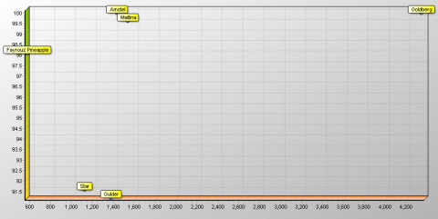
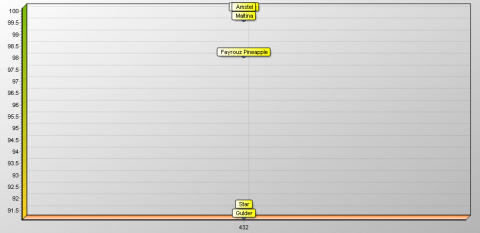
However, using the additive DEA model, and from the efficiency plot shown in Figure 1, relative to the actual production time, the Fayrouz pineapple used less production time to achieve an efficiency of about 98%. However, Goldberg obtained an efficiency of 100% but with a higher production time. Maltina being higher in the number of products is expected to have a higher efficiency score than Amstel, however, Amstel production (100%) used less production time compared to Maltina production line (99.5%) as shown in Figure 1. Manpower input for all the production lines is the same, however, from Figure 2, Amstel and Goldberg achieved an efficiency of 100% relative to the manpower used.
Table 2. Relative efficiency
|
Unit |
Actual Prod Time (APT)(Hr) |
Manpower (M) |
Products (P) (00,000) |
|
Gulder |
1376.70 |
432 |
337.181 |
|
Star |
1125.39 |
432 |
276.807 |
|
Goldberg |
4349.36 |
432 |
1092.523 |
|
Amstel |
1436.84 |
432 |
385.875 |
|
Maltina |
1541.84 |
432 |
409.745 |
|
Fayrouz Pineapple |
578.68 |
432 |
152.420 |
Figure 1. Efficiency plot (relative to actual production time)
Figure 2. Efficiency plot (relative to manpower)
The result revealed that out of the six production lines, two are the most efficient (has an efficiency score of 100%). One of these was made the benchmark to which others were compared. Also, Table 3 shows the efficiency scores of each of the units. It was observed that two of the six units utilized input resources to optimally produce the system output.
Table 3. Unit efficiency
|
Units |
Comparison 1 |
||
|
Unit name |
Score |
Efficient |
Condition |
|
Amstel |
100.0% |
√ |
⚪ |
|
Fayrouz Pineapple |
98.1% |
|
⚪ |
|
Goldberg |
100.0% |
√ |
⚪ |
|
Gulder |
91.2% |
|
⚪ |
|
Maltina |
99.6% |
|
⚪ |
|
Star |
91.6% |
|
⚪ |
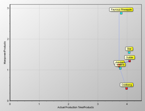
4.1 Production frontier plot
This reveals the efficiencies of the efficient units and to what extent the inefficient units lag compared to the benchmark. This reveals the ratio of inputs to output in the output maximization problem. This is shown in Figure 3.
Figure 3. Production frontier plot
4.2 Potential improvement and evaluation
For all the production lines considered and their inputs with their respective outputs, the percentage to which inputs or output can be improved to achieve the efficiency of the benchmark are described for each unit as follows:
4.2.1 Gulder
Table 4 shows the potential improvement in the input and output of the Gulder production line.
Table 4. Potential improvement (gulder)
|
Efficiency = 91.20% |
|
|
|
|
Variable |
Actual |
Target |
Potential improvement |
|
Actual Production Time |
1376.7 |
1376.7 |
0.00% |
|
Manpower |
432 |
413.92 |
-4.19% |
|
Products |
337.18 |
369.72 |
9.65% |
For this production line to meet up with the relative efficiency of the benchmark, the manpower should be decreased by 4.19%. Out of a total of 432 personnel on the line for a whole year, approximate 414 personnel be made to run the shifts for a year. Also, the units of products produced should be increased by 9.65% to meet up with the benchmark. This means that approximate 37,000,000 units of products are expected to be produced to meet up with the efficiency of the benchmark.
4.2.2 Star
Shown in Table 5 is the potential improvement in the input and output in the Star production line.
For the Star production line to meet up with the relative efficiency of the benchmark, the manpower should be decreased by 21.68%. Out of a total of 432 personnel on the line for a whole year, approximate 338 personnel be made to run the four shifts for a year on this line. Also, the units of products produced should be increased by 9.19% to meet up with the benchmark. This means that approximately 30, 224,884 units of products are expected to be produced to meet up with the efficiency of the benchmark.
Table 5. Potential improvement (star)
|
Efficiency = 91.59% Star |
|
|
|
|
Variable |
Actual |
Target |
Potential improvement |
|
Actual Production Time |
1125.39 |
1125.39 |
0.00% |
|
Manpower |
432 |
338.36 |
-21.68% |
|
Products |
276.81 |
302.23 |
9.19% |
4.2.3 Maltina
Shown in Table 6 is the improvement potential for Maltina production line.
Table 6. Potential improvement (maltina)
|
Efficiency = 99.61% |
|
|
|
|
Variable |
Actual |
Target |
Potential improvement |
|
Actual Production Time |
1541.84 |
1541.84 |
0.00% |
|
Manpower |
432 |
432 |
0.00% |
|
Products |
409.74 |
411.35 |
0.39% |
For the Maltina production line to meet up with the relative efficiency of the benchmark, the manpower was efficiently utilized. However, the units of products produced should be increased by 0.39% to meet up with the benchmark. This means that approximately 41,133,799 units of products are expected to be produced to meet up with the efficiency of the benchmark.
4.2.4 Fayrouz pineapple
Shown in Table 7 is the improvement potential for the Fayrouz Pineapple production line.
Table 7. Potential improvement (fayrouz pineapple)
|
Efficiency = 98.08% Fayrouz Pineapple |
|
||
|
Variable |
Actual |
Target |
Potential improvement |
|
Actual Production Time |
578.68 |
578.68 |
0.00% |
|
Manpower |
432 |
173.99 |
-59.73% |
|
Products |
152.42 |
155.41 |
1.96% |
For this production line to meet up with the relative efficiency of the benchmark the manpower should be decreased by 59.73%. Out of a total of 432 personnel on the line for a whole year, approximately 174 personnel be made to run the four shifts for a year on this line. Also, the units of products produced should be increased by 1.96% to meet up with the benchmark. This means that approximately 15,541,000 units of products are expected to be produced to meet up with the efficiency of the benchmark.
Performance measurement of decision units in manufacturing industries is fast becoming a concern. In response to this, several techniques are being developed both parametric and non-parametric measures. These methods are being adopted by both researchers and management to evaluate production systems. Data envelopment analysis (DEA) is one of the non-parametric measures of a production system where dimensional inconsistency does not affect output.
Some production lines often appear productive to management, however, when subjected to specific analysis may prove less efficient compared to others in the same system. Two inputs and one output were considered in this analysis: the manpower and actual production time, and the number of products respectively. It was observed that some production lines have more of these inputs than required by the number of products produced per time. This can be seen in the case of product F, product B as well as product A production lines which have more manpower than required. In contrast, some other product lines are observed to be producing less than the most efficient production line. This is the case of product A, product B, product F and product E production line which produces 9.65%, 9.19%, 1.96% and 0.39% respectively less than the most efficient production line.
Additionally, waste in the aspect of manpower is predominant in the system analysed. There is more of the production workforce than necessary compared to the capacity of the plant. To address this, the following recommendations were made that can aid management in decision-making. Even though investment in the area of skills has been made in the workforce in this production system. It is therefore expedient that the excess workforce should be laid off or another product line is created to which they can be deployed based on the desired production level. If considering the financial status of the industry, the man-hour cost of the excess workforce cannot be afforded by the industry, laying off the excess workforce could be a decision that can only be guided through continuous evaluation for performance improvement.
Production Time Per Month
Product A
|
Month |
Actual production time |
Manpower |
Products |
|
January |
234.06 |
36 |
4818564 |
|
February |
132.02 |
36 |
3193968 |
|
March |
125.31 |
36 |
3212100 |
|
April |
31.39 |
36 |
841560 |
|
May |
80.25 |
36 |
2029044 |
|
June |
124.38 |
36 |
3326388 |
|
July |
56.56 |
36 |
1383912 |
|
August |
113.01 |
36 |
2509896 |
|
September |
227.68 |
36 |
6005328 |
|
October |
29.43 |
36 |
720360 |
|
November |
74.24 |
36 |
1863012 |
|
December |
148.37 |
36 |
3813972 |
Product B Production Line
|
Month |
Actual production time |
Manpower |
Products |
|
January |
122.04 |
36 |
2512344 |
|
February |
140.63 |
36 |
3402276 |
|
March |
50.88 |
36 |
1304136 |
|
April |
49.83 |
36 |
1335852 |
|
May |
85.58 |
36 |
2163696 |
|
June |
79.29 |
36 |
2120508 |
|
July |
180.29 |
36 |
4411152 |
|
August |
17.4 |
36 |
386400 |
|
September |
74.64 |
36 |
1968768 |
|
October |
194.59 |
36 |
4762908 |
|
November |
57.19 |
36 |
1435356 |
|
December |
73.03 |
36 |
1877304 |
Product C Production Line
|
Month |
Actual production time |
Manpower |
Products |
|
January |
283.68 |
36 |
5840088 |
|
February |
299.22 |
36 |
7239336 |
|
March |
418.74 |
36 |
10734000 |
|
April |
515.5 |
36 |
13819848 |
|
May |
501.83 |
36 |
12687708 |
|
June |
424.33 |
36 |
11347920 |
|
July |
244.16 |
36 |
5973912 |
|
August |
159.24 |
36 |
3536436 |
|
September |
293.95 |
36 |
7753212 |
|
October |
413.89 |
36 |
10130676 |
|
November |
398.08 |
36 |
9990324 |
|
December |
396.74 |
36 |
10198848 |
Product D Production Line
|
Month |
Actual production time |
Manpower |
Products |
|
January |
101.23 |
36 |
2479248 |
|
February |
148.29 |
36 |
3691752 |
|
March |
85.84 |
36 |
2297496 |
|
April |
101.11 |
36 |
2663136 |
|
May |
130.71 |
36 |
3303528 |
|
June |
158.03 |
36 |
4496592 |
|
July |
90.13 |
36 |
2592048 |
|
August |
83.98 |
36 |
2256768 |
|
September |
40.15 |
36 |
988656 |
|
October |
123.5 |
36 |
3118968 |
|
November |
121.57 |
36 |
3246528 |
|
December |
252.3 |
36 |
7452744 |
Product E Production Line
|
Month |
Actual production time |
Manpower |
Products |
|
January |
249.53 |
36 |
6111072 |
|
February |
114.34 |
36 |
2846736 |
|
March |
106.16 |
36 |
2841336 |
|
April |
76.37 |
36 |
2011512 |
|
May |
136.44 |
36 |
3448368 |
|
June |
170.8 |
36 |
4859736 |
|
July |
68.94 |
36 |
1982592 |
|
August |
116.34 |
36 |
3126312 |
|
September |
43.86 |
36 |
1079832 |
|
October |
68.95 |
36 |
1741152 |
|
November |
206.81 |
36 |
5522712 |
|
December |
183.3 |
36 |
5403096 |
Product F
|
Month |
Actual production time |
Manpower |
Products |
|
January |
55.33 |
36 |
1355136 |
|
February |
25.68 |
36 |
639408 |
|
March |
50.47 |
36 |
1350792 |
|
April |
42.43 |
36 |
1117632 |
|
May |
50.26 |
36 |
1270200 |
|
June |
47.37 |
36 |
1347816 |
|
July |
91.52 |
36 |
2631912 |
|
August |
0 |
36 |
0 |
|
September |
42.43 |
36 |
1044720 |
|
October |
35.9 |
36 |
906528 |
|
November |
94.86 |
36 |
2533176 |
|
December |
42.43 |
36 |
1044720 |
[1] Bhagavath, V. (2006). Technical efficiency measurement by data envelopment analysis: An application in transportation. Allinace Journal of Business Research, 60-72.
[2] Adan, I.J.B.F., Hofkamp, A.T. (2012). Analysis of Manufacturing Systems: Using Chi 3.0. Technische Universiteit Eindhoven.
[3] Harvey, J. (2008). Performance Measurement. United Kingdom: CIMA.
[4] Wojcik, V., Dyckhoff, H., Clermont, M. (2019). Is data envelopment analysis a suitable tool for performance measurement and benchmarking in non-production contexts? Business Research, 12(2): 559-595. https://doi.org/10.1007/s40685-018-0077-z
[5] Sexton, T.R. (1986). Measuring Efficiency: An Assessment of DEA. In R. Silkman (Ed.), The Methodology of DEA, pp. 7-29. San Francisco: Jossey-Bass.
[6] Kao, C. (2014). Network data envelopment analysis: A review. European Journal of Operational Research, 239(1): 1-16. https://doi.org/10.1016/j.ejor.2014.02.039
[7] Cooper, W.W., Seiford, L.M., Tone, K. (2007). Data envelopment analysis: A comprehensive text with models, applications, references and DEA-solver software. In Data Envelopment Analysis, Vol. 2, p. 489. New York: Springer. https://doi.org/10.1007/b109347
[8] Azad, M.A.K., Teng, K.K., Talib, M.B.A. (2017). Modeling bank efficiency with bad output and network data envelopment analysis approach. Anadolu International Conference in Economics V, pp. 1-20.
[9] Othman, F.M., Mohd-Zamil, N.A., Rasid, S.Z.A., Vakilbashi, A., Mokhber, M. (2016). Data envelopment analysis: A tool of measuring efficiency in banking sector. International Journal of Economics and Financial Issues, 6(3): 911-916.
[10] Manninen, P. (2008). Performance Measurement Tools and Techniques. Sweden: CSC.
[11] Brønn, C., Brønn, P.S. (2005). Reputation and organizational efficiency: A data envelopment analysis study. Corporate Reputation Review, 8(1): 45-58.
[12] Ohio Department of Education. (2003). Introduction to Performance Measurement. Ohio: Ohio Department of Education.
[13] Barney, J. (1996). Gaining and Sustaining Competitive Advantage. Reading, M.A.: Addison-Wesley Publishing.
[14] Anderson, P., Peterson, N.C. (1993). A procedure for raking efficient units in DEA. Management Science, 39(10): 1261-1264. https://doi.org/10.1287/mnsc.39.10.1261
[15] Vincova, I.K. (2005). Using DEA to Measure Efficiency. Slovenska.
[16] Banker, R.D., Cooper, W.W., Seiford, L.M., Zhu, J. (2004). Returns to scale in different DEA models. European Journal of Operational Research, 154(2): 345-362. https://doi.org/10.1016/S0377-2217(03)00174-7
[17] Charnes, A., Cooper, W.W., Rhodes, E. (1978). Measuring the efficiency of DMUs. European Journal of Operations Research, 2(6): 429-444. https://doi.org/10.1016/0377-2217(78)90138-8
[18] Ramanathan, R. (2003). An Introduction to Data Envelopment Analysis: A Tool for Performance Measurement (1st ed.). London: Sage Publications Ltd.
[19] Australia. Steering Committee for the Review of Commonwealth/State Service Provision, Scales, B. (1997). Data envelopment analysis: A technique for measuring the efficiency of government service delivery. Industry Commission.
[20] Ozcan, Y.A. (2014). An Assessment Using Data Envelopment Analysis (DEA). In Health Care Benchmarking and Performance Evaluation, pp. 15-46. New York: Springer Science+Business Media.
[21] Banker, R.D., Charnes, A., Cooper, W.W. (1984). Some models for estimating technical and scale inefficiencies in data envelopment analysis. Management Science, 30(9): 1078-1092. https://doi.org/10.1287/mnsc.30.9.1078
[22] Cvetkoska, V. (2011). Data Envelopment Analysis Approach and Its Application in Information and Communication Technologies. Skiathos: International Conference on Information and Communication Technologies.
[23] Laskowska, J. (2011). Personal Controlling as a Management tool for library staff in the example of selected Polish Libraries. Library Management, 32(6-7): 475-468. https://doi.org/10.1108/01435121111158592
[24] Sherman, H.D., Zhu, J. (2006). Service Productivity Management: Improving Service Performance Using Data Envelopment Analysis. New York: Springer. https://doi.org/10.1007/0-387-33231-6
[25] Pesenti, R., Ukovich, W. (1996). Data Envelopment Analysis: A Possible way to Evaluate the Academic Activities. DEEI, Universita di Trieste.
[26] Ouenniche, J., Tone, K. (2017). An out-of-sample evaluation framework for DEA with application in bankruptcy prediction. Annals of Operations Research, 254: 235-250. https://doi.org/10.1007/s10479-017-2431-5
[27] Emrouznejad, A., Rostami-Tabar, B., Petridis, K. (2016). A novel ranking procedure for forecasting approaches using data envelopment analysis. Technological Forecasting and Social Change, 111: 235-243. https://doi.org/10.1016/j.techfore.2016.07.004
[28] Brazdil, P.B., Soares, C., Da Costa, J.P. (2003). Ranking learning algorithms: Using IBL and meta-learning on accuracy and time results. Machine Learning, 50: 251-277. https://doi.org/10.1023/A:1021713901879
[29] Tran, K.D., Bhaskar, A., Bunker, J., Lee, B. (2016). Data envelopment analysis (DEA) based transit route temporal performance assessment: A pilot study. In Australasian Transport Research Forum 2016 Proceedings, Australasian Transport Research Forum, pp. 1-18.
[30] Georgiadis, G., Politis, I., Papaioannou, P. (2014). Measuring and improving the efficiency and effectiveness of bus and public transport systems. Research in Transportation Economics, 48: 84-91. https://doi.org/10.1016/j.retrec.2014.09.035
[31] Monika, D., Mariana, S. (2015). The using of data envelopment analysis in human resource controlling. Procedia Economics and Finance, 26: 468-475. https://doi.org/10.1016/S2212-5671(15)00875-8
[32] Zhou, P., Poh, K.L., Ang, B.W. (2016). Data envelopment analysis for measuring environmental performance. In: Hwang, SN., Lee, HS., Zhu, J. (eds) Handbook of Operations Analytics Using Data Envelopment Analysis. International Series in Operations Research & Management Science, vol. 239. Springer, Boston, MA. https://doi.org/10.1007/978-1-4899-7705-2_2
[33] Zhu, J., Cook, W.D. (2007). Modeling Data Irregularities and Structural Complexities in Data Envelopment Analysis. New York: Springer. https://doi.org/10.1007/978-0-387-71607-7
[34] Zou, J., Chen, W., Peng, N., Wei, X. (2020). Efficiency of two-stage technological innovation in high patent-intensive industries that considers time lag: Research based on the SBM-NDEA model. Mathematical Problems in Engineering, 2020: 1-9. https://doi.org/10.1155/2020/2906293
[35] Villa, G., Lozano, S., Redondo, S. (2021). Data envelopment analysis approach to energy-saving projects selection in an energy service company. Mathematics, 9(2): 200. https://doi.org/10.3390/math9020200
[36] Fenyves, V., Tarnóczi, T. (2020). Data envelopment analysis for measuring performance in a competitive market. Problems and Perspectives in Management, 18(1): 315-325. http://dx.doi.org/10.21511/ppm.18(1).2020.27
[37] González-de-Julián, S., Barrachina-Martínez, I., Vivas-Consuelo, D., Bonet-Pla, Á., Usó-Talamantes, R. (2021). Data envelopment analysis applications on primary health care using exogenous variables and health outcomes. Sustainability, 13(3): 1337. https://doi.org/10.3390/su13031337
[38] Dobrovič, J., Čabinová, V., Gallo, P., Partlová, P., Váchal, J., Balogová, B., Orgonáš, J. (2021). Application of the DEA model in tourism SMEs: an empirical study from Slovakia in the context of business sustainability. Sustainability, 13(13): 7422. https://doi.org/10.3390/su13137422