Rasaq A. Kazeem*![]() | Moses O. Petinrin
| Moses O. Petinrin![]() | Peter O. Akhigbe | Tien Chien Jen
| Peter O. Akhigbe | Tien Chien Jen![]() | Esther T. Akinlabi
| Esther T. Akinlabi![]() | Stephen A. Akinlabi
| Stephen A. Akinlabi![]() | Omolayo M. Ikumapayi
| Omolayo M. Ikumapayi![]()
© 2023 IIETA. This article is published by IIETA and is licensed under the CC BY 4.0 license (http://creativecommons.org/licenses/by/4.0/).
OPEN ACCESS
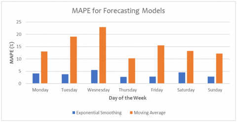
Starch-containing foods such as bread, pastries, and cakes are usually baked at a moderately high temperature in an oven. When these products are later exposed to room temperature, the associated gelatinized starch begins to harden which causes retrogradation and molecular realignment. Due to this circumstance, manufacturers need to have a fairly accurate estimate of products demand in order to determine the precise amount of baking powder and additives for use in their production so as not to incur losses in their business arising from the stale and consequentially unsalable products. This research was therefore focused on selecting the best forecasting model using a prominent confectionery firm in Abeokuta, Ogun State, Nigeria as a case study. The study was based on 24-week operational period sales data collected from the company. The moving average model and the exponential smoothing model were the two forecasting models considered in this research. The data obtained was thoroughly reviewed and the results of the forecasting models were compared. The most effective model was the exponential smoothing model as it produced the lowest mean absolute percentage error on the average of 3.7347 for the cumulative days of sales under review as against the 15.1713 for the moving average model. However, the exponential smoothing model was considered the best forecasting model for minimizing forecasting error in this study.
forecasting model, moving average model, exponential smoothing model, mean absolute percentage error
Making decisions requires a great deal of planning, strategy, and information [1]. Small bits of information have historically impacted the various segments of the manufacturing chain. Daily planning is crucial for management to make every significant decision [2]. Planning might take the form of determining the quantity needed, the quantity to be generated, and the storage methods [3]. The most crucial step we can take to increase the efficacy and efficiency of the logistics process in many supply chains is to raise the caliber of the demand forecasts. Using a planned marketing strategy and several unpredictable and competitive elements, demand forecasting estimates sales for a certain future time [4]. How much can be sold given the circumstances, it asks? The scenario considers the state of the general economic, social, and legal concerns, as well as the characteristics of vendors, buyers, and the market. The situation also involves the company's, its rivals', and interest groups' actions. Demand forecasting knowledge has advanced in the same way that science always does by accumulating data from tests of numerous plausible hypotheses in experiments [5]. Demand is the area where forecasting is most frequently employed, even though many products are projected. The demand projection will directly affect a wide range of business operations. Hugos [6] asserts that for every supplier, producer, or retailer, predicting product demand is essential. The amounts that should be ordered, produced, and shipped will be determined by forecasts of future demand. Forecasting demand is required because it takes time for finished items to get from the suppliers' raw materials to the customers' hands in the fundamental operational process. Most businesses are unable to simply wait for demand to materialize before acting on it. Instead, they must foresee and prepare for future demand to respond quickly to consumer orders as they come in. Forecasts give people power because it implies that we can change variables right now to change the future [7]. Higher productivity is the goal for every food-based sector, especially confectionaries, in terms of lowering production costs, increasing product demand, and maintaining competitiveness by lowering the cost of their varied products [8].
Even when sufficient care and professionalism are put into the efficient creation of the products in the manufacturing of bread, cakes, and confections, a poor profitability index is nevertheless seen. Retailers and vendors base their demand for bread on the amount of stock that is currently available as well as the amount of the prior stock that was sold because bread is a perishable product made from flour with a concise shelf life that must be consumed within the first 24 hours of production. The amount of the order cannot be guaranteed since, barring exceptional circumstances, the merchants must wait until the residual stock levels fall to an average of around 9% of the starting stock before placing an accurate order. The bakers rarely produce enough goods to meet demand since they are unsure of how many to order. Most of the time, they either produce less than what is required or less than what is required, which results in one of two outcomes: either significant loss for bakers and retailers because of underproduction or excessive production leading to waste because bread must be consumed within the first 24 hours of production (depreciation of product due to staleness). Both the stores and the bakeries ultimately suffer losses because of this. The need to reduce excessive manufacturing capacity, which will also reduce daily losses and shortages, maximize sales volume and profit margin, grow the client base, maintain high standards of quality, and boost the worth of the product, is essential. As a result, before production starts, the assurance of the actual demand quantity can be made available. Bakeries use their judgment on how much bread was sold the day before to estimate the quantity to be manufactured. Reliable projections must be made to ensure that the production amount is as close as feasible to the actual demand quantity [9]. Therefore, it is necessary to use forecasting methodologies to forecast the quantity of actual demand, thereby increasing sales and decreasing wastages and losses.
Businesses that give quick delivery to their clients tend to compel their market rivals to maintain completed product inventories to offer quick order turnaround times [10]. As a result, almost all organizations involved are required to produce or at the very least order parts following an estimate of future demand. Accurate demand forecasting also gives the company the chance to reduce costs by balancing manufacturing volumes, optimizing transportation, and generally organizing effective logistical operations. In general, correct demand projections result in operations that are efficient and provide high levels of customer service, while inaccurate forecasts invariably result in operations that are inefficient, expensive, and/or provide a low standard of customer service. Numerous studies have examined the use of various forecasting models in a variety of technical and industrial applications. Liu et al. [11] used the exponential smoothing and seasonal autoregressive integrated moving average models to anticipate the trend in the prevalence of acute hemorrhagic conjunctivitis in China from 2011 to 2019. Consequently, the moving model with the lowest mean absolute percentage error (MAPE) and root mean squared error (RMSE) was chosen for in-sample modeling. Also, Rabbani et al. [12] used univariate time series analysis, such as exponential smoothing and seasonal autoregressive integrated moving average models, to develop temporal variations to forecast accidents and fatalities in Pakistan. Upon determining the lowest RMSE, mean absolute error (MAE), MAPE, and normalized Bayesian estimation technique, the results showed that the exponential model fit perfectly on accident data than the moving average model. In predicting telecommunication data, Nalawade and Pawar [13] utilized an autoregressive integrated moving average model. This model utilized auto regression, moving average, or a mix of both. Using evaluation metrics such as RMSE, sum of squared regression, MAPE, mean absolute deviation (MAD), and maximum absolute error, it is possible to determine how well the model performs. The findings demonstrated that the accuracy of forecasting using autoregressive integrated moving average models is 7.6% better than that using neural network methods. Moreover, Jere et al. [14] compared the performance of Holt Winters exponential smoothing models (HWES) and auto-regressive integrated moving average. The error indicators including MAE, mean percentage error, RMSE, mean absolute scaled error, and MAPE demonstrated that HWES is a suitable model with adequate forecast accuracy. The HWES has lower error than the autoregressive integrated moving average models. In order to anticipate how changes in temperature would affect the amount of energy produced at a Nigerian Agricultural Institute, Kazeem et al. [15] used multivariate linear regression (MLR) and artificial neural network (ANN) models. Of the two models examined in this study, the ANN model performed the best. On train data and test data, respectively, the mean squared error was reduced by 42% and 39%, showing that ANNs outperformed the MLR model. The ANN fared noticeably better than the MLR, according to additional metrics like MAE and MAPE.
Most of the application of forecasting models in literature are centered on predicting future events in health, telecommunications, energy and agriculture but very little investigators had bothered on their use in confectionery forecasting. The study, therefore, aims to establish an effective and efficient model that will forecast how much is produced each day in the selected baking and confectionery company. Additionally, it will show how this approach is used in the sales and operations of the bakery and confections sector. The remaining part of this paper, which are in three sections have the data source, the procedure for data collation and forecasting models, and the performance statistics index as sub-headings in section 2. The results and discussion is presented in section 3. The conclusions is presented in section 4 of the paper.
2.1 Data source
The data used in this study were obtained from XXX Bakery and Confectionery located in Abeokuta, Southwestern, Nigeria. The company makes several varieties of confectionaries and baked items therefore, customers have a wide range of confectionaries to choose from. Confections include vanilla, chocolate, strawberry, and chicken pizza, chicken pie sausages, bread, and sponge cakes in flavors. The products come in a variety of sizes and shapes and are primarily divided into six main pricing ranges. However, there is variation in the demand for various products. The data derived from sales is transformed into a uniform size for simple data collecting, analysis, and interpretation. To select an acceptable forecasting model, the generated data will be employed. The data collected was for a period of one hundred and sixty-eight days (24 weeks). The data was collected physically and not from any National Scientific Data Sharing Platform.
2.2 Procedure
The first step in conducting this study was gathering and critically analyzing the sales and demand data for twenty-four weeks, after which appropriate alterations were made to suit the situation at hand. The next step was the application of the forecasting models that were considered when conducting this investigation. The forecasting models applied to the data include (i) The exponential smoothing model and (ii) The moving average model. Each technique used to apply these models to the sales data was closely examined for any errors, corrections, and modifications (mathematical, computational, data misevaluation, and formula or figure distortion) during the analysis. The model with the smallest divergence from the actual sales record was considered the best prediction approach for the company’s products.
2.2.1 Exponential smoothing model
The most utilized class of techniques for smoothing discrete time series to forecast the near future is exponential smoothing. The objective behind exponential smoothing is to smooth the original series in the same manner that the moving average does, then use the smoothed series to forecast future values of the variable of interest. However, in exponential smoothing, we want the more recent values of the series to have a higher influence on the forecast of future values than the more distant observations. Weighted averages are used to calculate forecasts, and as observations are gathered from further in the past, the weights decline exponentially, with the oldest observations having the smallest weights (see Eq. (1)):
$\left.\hat{y}_{T+1}\right|_T=\alpha y_T+\alpha(1-\alpha) y_{T-1}+\alpha(1-\alpha)^2 y_{T-2}+\ldots$, (1)
where, 0≤α≤1 is the smoothing parameter. The one-step-ahead forecast for time T+1 is a weighted average of all the observations in the series y1…, yT. The rate at which the weights decrease is controlled by the parameter α. Formally, the exponential smoothing equation employed is given in Eq. (2).
$y_{T+\left.1\right|_T}=\alpha y_T+(1-\alpha) \hat{y}_{\left.T\right|_{T-1}}$ (2)
where, yT+1/T=forecast for the next period; yT=observed sales value of series in period t; α=smoothing constant; and $\hat{y}_{T / T-1}$=old forecast for period t.
2.2.2 Moving average model
The simple moving average (SMA) method is used with time-series data to smooth out short-term fluctuations and long-term trends. The simple moving average is given by Eq. (3).
$S M A_k=\frac{P_{n-k+1}+P_{n-k+2} \ldots+P_n}{k}=\frac{1}{k} \sum_{i=n-k+1}^n P_i$ (3)
When calculating the next mean SMAk, nextwith the same sampling width k the range from n=k+2 to n+1 is considered. A new value Pn+1 comes into the sum and the oldest value $P_{n-k+1}$ drops out. This simplifies the calculations by reusing the previous mean SMAk, prev shown in Eq. (4).
$S M A_{k,next }=\frac{1}{k} \sum_{i=n-k+2}^{n+1} P_i=\frac{1}{k}\left(\underbrace{P_{n-k+2}+P_{n-k+3}+\ldots . .+P_n+P_{n+1}}_{\sum_{i=n-k+2}^{n+1}\quad P_i}+\underbrace{P_{n-k+1}-P_{n-k+1}}_0 \right)$ (4)
2.3 Performance statistic index
To compare the predicting capabilities of the exponential smoothing model and the moving average model, one metric was used: the mean absolute percentage error (MAPE). The accuracy of fitting was evaluated using MAPE [16]. The lower the MAPE value, the greater the prediction ability. MAPE is expressed as a percentage. The mathematical formula is shown in Eq. (5).
$M A P E=\frac{1}{n} \sum_{t=1}^n \frac{\left\|\hat{y}_t-y_t\right\|}{y_t} \times 100 \%$ (5)
where, yt-actual sales at time t; $\hat{y}_t$-predicted sales; n-number of predictions.
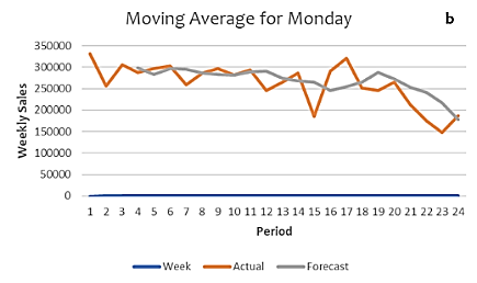
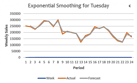
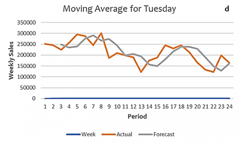
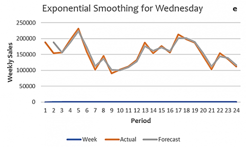
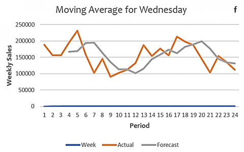
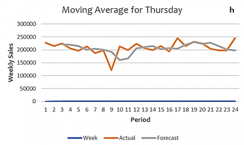
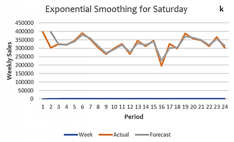
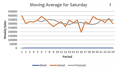
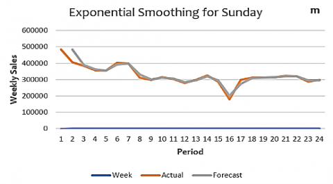
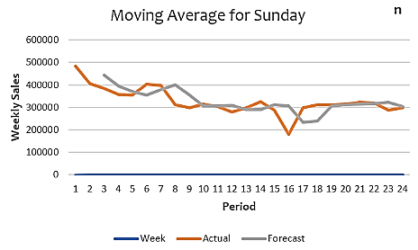
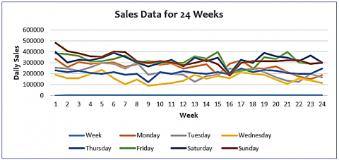
The data were collected from the company’s daily sales and are represented as shown in Table 1. The model applications and analysis are presented in Tables 2-15, and subsequently, the forecasts with the least MAPE for each day were plotted against the actual sales values as shown in Figures 1 (a-n). The data in Table 1 is better appreciated in the graph provided in Figure 2. According to sales statistics, the company sold more goodies on the weekends and had poor sales during the middle of the week because most customers had free time on the weekends and were extremely busy during the middle of the work week. The weekly trend in sales also show a downward trend in sales. Moreover, an outside factor that influences the company's sales demand is the seasonal effect. Also, the strike action of the flour-producing companies in the country was said to have affected the supply of flour for production in their establishment and this invariably caused the fluctuation among some days in the data provided. Another cause of sales drops in some of the days was attributed to price increase of petroleum products and epileptic power supply which therefore caused price increases of the company's goods. Generally, sales are often higher on weekends than on weekdays and are at their lowest on Wednesdays. As computed in the last column of the Table 1 for the average weekly sales and the spread of daily sales across the 24 weeks shown in Table 1. Figure 1 shows that the trend in the sales data for each day of the study period was not linear, making it impossible to use linear regression [17, 18]. However, it could be deduced form this figure and as indicated in the last column of Table 1, that the sales are badly affected from the early weeks of data collection, and this trend continues till the end of the twenty-fourth week. As it was mentioned earlier, the trend in reduced sales was unconnected with hike in the price of petroleum products, which are mostly used in transportation, and production of goods. This reduced production of confections, and there was also low demand from customers arising from market inflation, which reduces the purchasing power of the customers.
(a)
(b)
(c)
(d)
(e)
(f)
(g)
(h)
(i)
(j)
(k)
(l)
(m)
(n)
Figure 1. (a-n): Comparison of forecasting models for weekly sales data
Table 1. Daily sales data for twenty-four weeks
|
Week |
Monday |
Tuesday |
Wednesday |
Thursday |
Friday |
Saturday |
Sunday |
Weekly Average |
|
1 |
331200 |
251400 |
188750 |
227580 |
385500 |
397500 |
482500 |
323490 |
|
2 |
256600 |
245200 |
156400 |
214600 |
375400 |
302500 |
405000 |
279386 |
|
3 |
305450 |
224500 |
156400 |
224500 |
360000 |
325500 |
385000 |
283050 |
|
4 |
287500 |
256000 |
195000 |
205000 |
308000 |
320000 |
356000 |
275357 |
|
5 |
297500 |
295400 |
231000 |
196000 |
312500 |
345000 |
355000 |
290343 |
|
6 |
302500 |
287500 |
158000 |
213500 |
333500 |
389000 |
402500 |
298071 |
|
7 |
259500 |
245600 |
102300 |
187000 |
365000 |
352000 |
397000 |
272629 |
|
8 |
287000 |
302000 |
145600 |
198400 |
297500 |
302000 |
312500 |
263571 |
|
9 |
297000 |
187500 |
90540 |
121500 |
312500 |
264880 |
298740 |
224666 |
|
10 |
282500 |
210330 |
102300 |
213000 |
301230 |
298700 |
315000 |
246151 |
|
11 |
294000 |
198750 |
112300 |
198800 |
302540 |
325400 |
302500 |
247756 |
|
12 |
245660 |
189700 |
132500 |
223000 |
298700 |
265000 |
278900 |
233351 |
|
13 |
265000 |
123000 |
187900 |
206500 |
356400 |
345600 |
298700 |
254729 |
|
14 |
287000 |
175640 |
154600 |
198700 |
335640 |
312540 |
325600 |
255674 |
|
15 |
185000 |
187900 |
177000 |
214500 |
397000 |
345600 |
287000 |
256286 |
|
16 |
290500 |
245600 |
156400 |
194500 |
198700 |
196540 |
178900 |
208734 |
|
17 |
320200 |
231200 |
213000 |
245100 |
225780 |
325460 |
298970 |
265673 |
|
18 |
251000 |
245800 |
198000 |
214500 |
235460 |
298750 |
312000 |
250787 |
|
19 |
245000 |
214000 |
187000 |
231450 |
348790 |
387500 |
312540 |
275183 |
|
20 |
265400 |
165400 |
145600 |
224500 |
332540 |
356470 |
314500 |
257773 |
|
21 |
212000 |
132540 |
103200 |
204500 |
398700 |
346500 |
321500 |
245563 |
|
22 |
174500 |
123000 |
154600 |
198400 |
302500 |
312500 |
320540 |
226577 |
|
23 |
147800 |
198700 |
135600 |
197800 |
287500 |
365400 |
287950 |
231536 |
|
24 |
186500 |
165020 |
112300 |
245600 |
302540 |
302540 |
298750 |
230464 |
Table 2. Analysis of Monday data using exponential smoothing method
|
Exponential Smoothing for Monday |
MAPE |
||||||||
|
Week |
Monday |
α= 0.2 |
α= 0.4 |
α= 0.6 |
α= 0.8 |
0.2 |
0.4 |
0.6 |
0.8 |
|
1 |
331200 |
|
|
|
|
|
|
|
|
|
2 |
256600 |
331200 |
331200 |
331200 |
331200 |
29.07248636 |
29.07248636 |
29.07248636 |
29.07248636 |
|
3 |
305450 |
266370 |
276140 |
285910 |
295680 |
12.79423801 |
9.595678507 |
6.397119005 |
3.198559502 |
|
4 |
287500 |
301860 |
298270 |
294680 |
291090 |
4.994782609 |
3.746086957 |
2.497391304 |
1.248695652 |
|
5 |
297500 |
289500 |
291500 |
293500 |
295500 |
2.68907563 |
2.016806723 |
1.344537815 |
0.672268908 |
|
6 |
302500 |
298500 |
299500 |
300500 |
301500 |
1.32231405 |
0.991735537 |
0.661157025 |
0.330578512 |
|
7 |
259500 |
293900 |
285300 |
276700 |
268100 |
13.25626204 |
9.942196532 |
6.628131021 |
3.314065511 |
|
8 |
287000 |
265000 |
270500 |
276000 |
281500 |
7.665505226 |
5.74912892 |
3.832752613 |
1.916376307 |
|
9 |
297000 |
289000 |
291000 |
293000 |
295000 |
2.693602694 |
2.02020202 |
1.346801347 |
0.673400673 |
|
10 |
282500 |
294100 |
291200 |
288300 |
285400 |
4.10619469 |
3.079646018 |
2.053097345 |
1.026548673 |
|
11 |
294000 |
284800 |
287100 |
289400 |
291700 |
3.129251701 |
2.346938776 |
1.56462585 |
0.782312925 |
|
12 |
245660 |
284332 |
274664 |
264996 |
255328 |
15.74208255 |
11.80656191 |
7.871041277 |
3.935520638 |
|
13 |
265000 |
249528 |
253396 |
257264 |
261132 |
5.838490566 |
4.378867925 |
2.919245283 |
1.459622642 |
|
14 |
287000 |
269400 |
273800 |
278200 |
282600 |
6.132404181 |
4.599303136 |
3.066202091 |
1.533101045 |
|
15 |
185000 |
266600 |
246200 |
225800 |
205400 |
44.10810811 |
33.08108108 |
22.05405405 |
11.02702703 |
|
16 |
290500 |
206100 |
227200 |
248300 |
269400 |
29.05335628 |
21.79001721 |
14.52667814 |
7.263339071 |
|
17 |
320200 |
296440 |
302380 |
308320 |
314260 |
7.420362274 |
5.565271705 |
3.710181137 |
1.855090568 |
|
18 |
251000 |
306360 |
292520 |
278680 |
264840 |
22.05577689 |
16.54183267 |
11.02788845 |
5.513944223 |
|
19 |
245000 |
249800 |
248600 |
247400 |
246200 |
1.959183673 |
1.469387755 |
0.979591837 |
0.489795918 |
|
20 |
265400 |
249080 |
253160 |
257240 |
261320 |
6.149208742 |
4.611906556 |
3.074604371 |
1.537302185 |
|
21 |
212000 |
254720 |
244040 |
233360 |
222680 |
20.1509434 |
15.11320755 |
10.0754717 |
5.037735849 |
|
22 |
174500 |
204500 |
197000 |
189500 |
182000 |
17.19197708 |
12.89398281 |
8.595988539 |
4.297994269 |
|
23 |
147800 |
169160 |
163820 |
158480 |
153140 |
14.45196211 |
10.83897158 |
7.225981055 |
3.612990528 |
|
24 |
186500 |
155540 |
163280 |
171020 |
178760 |
16.60053619 |
12.45040214 |
8.300268097 |
4.150134048 |
|
|
|
|
|
|
Sum |
288.5781051 |
223.7017004 |
158.8252957 |
93.94889104 |
|
|
|
|
|
|
Mean |
12.54687413 |
9.726160886 |
6.90544764 |
4.084734393 |
Table 3. Analysis of Tuesday data using exponential smoothing method
|
Exponential Smoothing for Tuesday |
MAPE |
||||||||
|
Week |
Tuesday |
α= 0.2 |
α= 0.4 |
α= 0.6 |
α= 0.8 |
0.2 |
0.4 |
0.6 |
0.8 |
|
1 |
251400 |
|
|
|
|
|
|
|
|
|
2 |
245200 |
251400 |
251400 |
251400 |
251400 |
2.528548124 |
2.528548124 |
2.528548124 |
2.528548124 |
|
3 |
224500 |
241060 |
236920 |
232780 |
228640 |
7.376391982 |
5.532293987 |
3.688195991 |
1.844097996 |
|
4 |
256000 |
230800 |
237100 |
243400 |
249700 |
9.84375 |
7.3828125 |
4.921875 |
2.4609375 |
|
5 |
295400 |
263880 |
271760 |
279640 |
287520 |
10.67027759 |
8.002708192 |
5.335138795 |
2.667569397 |
|
6 |
287500 |
293820 |
292240 |
290660 |
289080 |
2.19826087 |
1.648695652 |
1.099130435 |
0.549565217 |
|
7 |
245600 |
279120 |
270740 |
262360 |
253980 |
13.64820847 |
10.23615635 |
6.824104235 |
3.412052117 |
|
8 |
302000 |
256880 |
268160 |
279440 |
290720 |
14.94039735 |
11.20529801 |
7.470198675 |
3.735099338 |
|
9 |
187500 |
279100 |
256200 |
233300 |
210400 |
48.85333333 |
36.64 |
24.42666667 |
12.21333333 |
|
10 |
210330 |
192066 |
196632 |
201198 |
205764 |
8.683497361 |
6.512623021 |
4.341748681 |
2.17087434 |
|
11 |
198750 |
208014 |
205698 |
203382 |
201066 |
4.661132075 |
3.495849057 |
2.330566038 |
1.165283019 |
|
12 |
189700 |
196940 |
195130 |
193320 |
191510 |
3.816552451 |
2.862414338 |
1.908276226 |
0.954138113 |
|
13 |
123000 |
176360 |
163020 |
149680 |
136340 |
43.38211382 |
32.53658537 |
21.69105691 |
10.84552846 |
|
14 |
175640 |
133528 |
144056 |
154584 |
165112 |
23.97631519 |
17.98223639 |
11.9881576 |
5.994078798 |
|
15 |
187900 |
178092 |
180544 |
182996 |
185448 |
5.219797765 |
3.914848324 |
2.609898882 |
1.304949441 |
|
16 |
245600 |
199440 |
210980 |
222520 |
234060 |
18.79478827 |
14.09609121 |
9.397394137 |
4.698697068 |
|
17 |
231200 |
242720 |
239840 |
236960 |
234080 |
4.982698962 |
3.737024221 |
2.491349481 |
1.24567474 |
|
18 |
245800 |
234120 |
237040 |
239960 |
242880 |
4.751830757 |
3.563873068 |
2.375915378 |
1.187957689 |
|
19 |
214000 |
239440 |
233080 |
226720 |
220360 |
11.88785047 |
8.91588785 |
5.943925234 |
2.971962617 |
|
20 |
165400 |
204280 |
194560 |
184840 |
175120 |
23.50665054 |
17.62998791 |
11.75332527 |
5.876662636 |
|
21 |
132540 |
158828 |
152256 |
145684 |
139112 |
19.83401237 |
14.87550928 |
9.917006187 |
4.958503093 |
|
22 |
123000 |
130632 |
128724 |
126816 |
124908 |
6.204878049 |
4.653658537 |
3.102439024 |
1.551219512 |
|
23 |
198700 |
138140 |
153280 |
168420 |
183560 |
30.4781077 |
22.85858078 |
15.23905385 |
7.619526925 |
|
24 |
165020 |
191964 |
185228 |
178492 |
171756 |
16.32771785 |
12.24578839 |
8.163858926 |
4.081929463 |
|
|
|
|
|
|
Sum |
336.5671114 |
253.0574706 |
169.5478297 |
86.03818893 |
|
|
|
|
|
|
Mean |
14.63335267 |
11.00249872 |
7.371644771 |
3.740790823 |
Table 4. Analysis of Wednesday data using exponential smoothing method
|
Exponential Smoothing for Wednesday |
MAPE |
||||||||
|
Week |
Wednesday |
α= 0.2 |
α= 0.4 |
α= 0.6 |
α= 0.8 |
0.2 |
0.4 |
0.6 |
0.8 |
|
1 |
188750 |
|
|
|
|
|
|
|
|
|
2 |
154220 |
188750 |
188750 |
188750 |
188750 |
22.3900921 |
22.3900921 |
22.3900921 |
22.39009208 |
|
3 |
156400 |
154656 |
155092 |
155528 |
155964 |
1.11508951 |
0.83631714 |
0.55754476 |
0.278772379 |
|
4 |
195000 |
164120 |
171840 |
179560 |
187280 |
15.8358974 |
11.8769231 |
7.91794872 |
3.958974359 |
|
5 |
231000 |
202200 |
209400 |
216600 |
223800 |
12.4675325 |
9.35064935 |
6.23376623 |
3.116883117 |
|
6 |
158000 |
216400 |
201800 |
187200 |
172600 |
36.9620253 |
27.721519 |
18.4810127 |
9.240506329 |
|
7 |
102300 |
146860 |
135720 |
124580 |
113440 |
43.5581623 |
32.6686217 |
21.7790811 |
10.88954057 |
|
8 |
145600 |
110960 |
119620 |
128280 |
136940 |
23.7912088 |
17.8434066 |
11.8956044 |
5.947802198 |
|
9 |
90540 |
134588 |
123576 |
112564 |
101552 |
48.6503203 |
36.4877402 |
24.3251602 |
12.16258008 |
|
10 |
102300 |
92892 |
95244 |
97596 |
99948 |
9.19648094 |
6.8973607 |
4.59824047 |
2.299120235 |
|
11 |
112300 |
104300 |
106300 |
108300 |
110300 |
7.1237756 |
5.3428317 |
3.5618878 |
1.7809439 |
|
12 |
132500 |
116340 |
120380 |
124420 |
128460 |
12.1962264 |
9.14716981 |
6.09811321 |
3.049056604 |
|
13 |
187900 |
143580 |
154660 |
165740 |
176820 |
23.5870144 |
17.6902608 |
11.7935072 |
5.896753592 |
|
14 |
154600 |
181240 |
174580 |
167920 |
161260 |
17.2315653 |
12.923674 |
8.61578266 |
4.307891332 |
|
15 |
177000 |
159080 |
163560 |
168040 |
172520 |
10.1242938 |
7.59322034 |
5.06214689 |
2.531073446 |
|
16 |
156400 |
172880 |
168760 |
164640 |
160520 |
10.5370844 |
7.9028133 |
5.2685422 |
2.6342711 |
|
17 |
213000 |
167720 |
179040 |
190360 |
201680 |
21.258216 |
15.943662 |
10.629108 |
5.314553991 |
|
18 |
198000 |
210000 |
207000 |
204000 |
201000 |
6.06060606 |
4.54545455 |
3.03030303 |
1.515151515 |
|
19 |
187000 |
195800 |
193600 |
191400 |
189200 |
4.70588235 |
3.52941176 |
2.35294118 |
1.176470588 |
|
20 |
145600 |
178720 |
170440 |
162160 |
153880 |
22.7472527 |
17.0604396 |
11.3736264 |
5.686813187 |
|
21 |
103200 |
137120 |
128640 |
120160 |
111680 |
32.8682171 |
24.6511628 |
16.4341085 |
8.217054264 |
|
22 |
154600 |
113480 |
123760 |
134040 |
144320 |
26.5976714 |
19.9482536 |
13.2988357 |
6.649417853 |
|
23 |
135600 |
150800 |
147000 |
143200 |
139400 |
11.2094395 |
8.40707965 |
5.60471976 |
2.802359882 |
|
24 |
112300 |
130940 |
126280 |
121620 |
116960 |
16.5983972 |
12.4487979 |
8.29919858 |
4.149599288 |
|
|
|
|
|
|
Sum |
436.812451 |
333.206861 |
229.601272 |
125.9956819 |
|
|
|
|
|
|
Mean |
18.9918457 |
14.4872548 |
9.98266399 |
5.478073125 |
Table 5. Analysis of Thursday data using exponential smoothing method
|
Exponential Smoothing for Thursday |
MAPE |
||||||||
|
Week |
Thursday |
α= 0.2 |
α= 0.4 |
α= 0.6 |
α= 0.8 |
0.2 |
0.4 |
0.6 |
0.8 |
|
1 |
227580 |
|
|
|
|
|
|
|
|
|
2 |
214600 |
227580 |
227580 |
227580 |
227580 |
6.048462 |
6.048462 |
6.048462 |
6.048462 |
|
3 |
224500 |
216580 |
218560 |
220540 |
222520 |
3.52784 |
2.64588 |
1.76392 |
0.88196 |
|
4 |
205000 |
220600 |
216700 |
212800 |
208900 |
7.609756 |
5.707317 |
3.804878 |
1.902439 |
|
5 |
196000 |
203200 |
201400 |
199600 |
197800 |
3.673469 |
2.755102 |
1.836735 |
0.918367 |
|
6 |
213500 |
199500 |
203000 |
206500 |
210000 |
6.557377 |
4.918033 |
3.278689 |
1.639344 |
|
7 |
187000 |
208200 |
202900 |
197600 |
192300 |
11.3369 |
8.502674 |
5.668449 |
2.834225 |
|
8 |
198400 |
189280 |
191560 |
193840 |
196120 |
4.596774 |
3.447581 |
2.298387 |
1.149194 |
|
9 |
121500 |
183020 |
167640 |
152260 |
136880 |
50.63374 |
37.97531 |
25.31687 |
12.65844 |
|
10 |
213000 |
139800 |
158100 |
176400 |
194700 |
34.3662 |
25.77465 |
17.1831 |
8.591549 |
|
11 |
198800 |
210160 |
207320 |
204480 |
201640 |
5.714286 |
4.285714 |
2.857143 |
1.428571 |
|
12 |
223000 |
203640 |
208480 |
213320 |
218160 |
8.681614 |
6.511211 |
4.340807 |
2.170404 |
|
13 |
206500 |
219700 |
216400 |
213100 |
209800 |
6.392252 |
4.794189 |
3.196126 |
1.598063 |
|
14 |
198700 |
204940 |
203380 |
201820 |
200260 |
3.140413 |
2.35531 |
1.570206 |
0.785103 |
|
15 |
214500 |
201860 |
205020 |
208180 |
211340 |
5.892774 |
4.41958 |
2.946387 |
1.473193 |
|
16 |
194500 |
210500 |
206500 |
202500 |
198500 |
8.226221 |
6.169666 |
4.113111 |
2.056555 |
|
17 |
245100 |
204620 |
214740 |
224860 |
234980 |
16.51571 |
12.38678 |
8.257854 |
4.128927 |
|
18 |
214500 |
238980 |
232860 |
226740 |
220620 |
11.41259 |
8.559441 |
5.706294 |
2.853147 |
|
19 |
231450 |
217890 |
221280 |
224670 |
228060 |
5.858717 |
4.394038 |
2.929358 |
1.464679 |
|
20 |
224500 |
230060 |
228670 |
227280 |
225890 |
2.476615 |
1.857461 |
1.238307 |
0.619154 |
|
21 |
204500 |
220500 |
216500 |
212500 |
208500 |
7.823961 |
5.867971 |
3.91198 |
1.95599 |
|
22 |
198400 |
203280 |
202060 |
200840 |
199620 |
2.459677 |
1.844758 |
1.229839 |
0.614919 |
|
23 |
197800 |
198280 |
198160 |
198040 |
197920 |
0.242669 |
0.182002 |
0.121335 |
0.060667 |
|
24 |
245600 |
207360 |
216920 |
226480 |
236040 |
15.57003 |
11.67752 |
7.785016 |
3.892508 |
|
|
|
|
|
|
Sum |
228.758 |
173.0806 |
117.4033 |
61.72586 |
|
|
|
|
|
|
Mean |
9.946002 |
7.525246 |
5.104489 |
2.683733 |
Table 6. Analysis of Friday data using exponential smoothing method
|
Exponential Smoothing for Friday |
MAPE |
||||||||
|
Week |
Friday |
α= 0.2 |
α= 0.4 |
α= 0.6 |
α= 0.8 |
0.2 |
0.4 |
0.6 |
0.8 |
|
1 |
385500 |
|
|
|
|
|
|
|
|
|
2 |
375400 |
385500 |
385500 |
385500 |
385500 |
2.690464 |
2.690463506 |
2.690463506 |
2.690463506 |
|
3 |
360000 |
372320 |
369240 |
366160 |
363080 |
3.422222 |
2.566666667 |
1.711111111 |
0.855555556 |
|
4 |
308000 |
349600 |
339200 |
328800 |
318400 |
13.50649 |
10.12987013 |
6.753246753 |
3.376623377 |
|
5 |
312500 |
308900 |
309800 |
310700 |
311600 |
1.152 |
0.864 |
0.576 |
0.288 |
|
6 |
333500 |
316700 |
320900 |
325100 |
329300 |
5.037481 |
3.778110945 |
2.51874063 |
1.259370315 |
|
7 |
365000 |
339800 |
346100 |
352400 |
358700 |
6.90411 |
5.178082192 |
3.452054795 |
1.726027397 |
|
8 |
297500 |
351500 |
338000 |
324500 |
311000 |
18.15126 |
13.61344538 |
9.075630252 |
4.537815126 |
|
9 |
312500 |
300500 |
303500 |
306500 |
309500 |
3.84 |
2.88 |
1.92 |
0.96 |
|
10 |
301230 |
310246 |
307992 |
305738 |
303484 |
2.993062 |
2.244796335 |
1.49653089 |
0.748265445 |
|
11 |
302540 |
301492 |
301754 |
302016 |
302278 |
0.3464 |
0.259800357 |
0.173200238 |
0.086600119 |
|
12 |
298700 |
301772 |
301004 |
300236 |
299468 |
1.028457 |
0.771342484 |
0.514228323 |
0.257114161 |
|
13 |
356400 |
310240 |
321780 |
333320 |
344860 |
12.95174 |
9.713804714 |
6.475869809 |
3.237934905 |
|
14 |
335640 |
352248 |
348096 |
343944 |
339792 |
4.948159 |
3.711119056 |
2.474079371 |
1.237039685 |
|
15 |
397000 |
347912 |
360184 |
372456 |
384728 |
12.36474 |
9.273551637 |
6.182367758 |
3.091183879 |
|
16 |
198700 |
357340 |
317680 |
278020 |
238360 |
79.83895 |
59.8792149 |
39.9194766 |
19.9597383 |
|
17 |
225780 |
204116 |
209532 |
214948 |
220364 |
9.595181 |
7.196385862 |
4.797590575 |
2.398795287 |
|
18 |
235460 |
227716 |
229652 |
231588 |
233524 |
3.288881 |
2.466661004 |
1.644440669 |
0.822220335 |
|
19 |
348790 |
258126 |
280792 |
303458 |
326124 |
25.99386 |
19.49539838 |
12.99693225 |
6.498466126 |
|
20 |
332540 |
345540 |
342290 |
339040 |
335790 |
3.909304 |
2.931978108 |
1.954652072 |
0.977326036 |
|
21 |
398700 |
345772 |
359004 |
372236 |
385468 |
13.27514 |
9.956358164 |
6.637572109 |
3.318786055 |
|
22 |
302500 |
379460 |
360220 |
340980 |
321740 |
25.44132 |
19.08099174 |
12.72066116 |
6.360330579 |
|
23 |
287500 |
299500 |
296500 |
293500 |
290500 |
4.173913 |
3.130434783 |
2.086956522 |
1.043478261 |
|
24 |
302540 |
290508 |
293516 |
291450 |
299121 |
5.122391 |
2.653425321 |
3.348750922 |
1.114736028 |
|
|
|
|
|
|
Sum |
254.8531 |
191.8124763 |
128.7718054 |
65.73113445 |
|
|
|
|
|
|
Mean |
11.08057 |
8.339672884 |
5.598774147 |
2.857875411 |
Table 7. Analysis of Saturday data using exponential smoothing method
|
Exponential Smoothing for Saturday |
MAPE |
||||||||
|
Week |
Saturday |
α= 0.2 |
α= 0.4 |
α= 0.6 |
α= 0.8 |
0.2 |
0.4 |
0.6 |
0.8 |
|
1 |
397500 |
|
|
|
|
|
|
|
|
|
2 |
302500 |
397500 |
397500 |
397500 |
397500 |
31.40496 |
31.40495868 |
31.40495868 |
31.40495868 |
|
3 |
325500 |
307100 |
311700 |
316300 |
320900 |
5.652842 |
4.239631336 |
2.826420891 |
1.413210445 |
|
4 |
320000 |
324400 |
323300 |
322200 |
321100 |
1.375 |
1.03125 |
0.6875 |
0.34375 |
|
5 |
345000 |
325000 |
330000 |
335000 |
340000 |
5.797101 |
4.347826087 |
2.898550725 |
1.449275362 |
|
6 |
389000 |
353800 |
362600 |
371400 |
380200 |
9.048843 |
6.786632391 |
4.524421594 |
2.262210797 |
|
7 |
352000 |
381600 |
374200 |
366800 |
359400 |
8.409091 |
6.306818182 |
4.204545455 |
2.102272727 |
|
8 |
302000 |
342000 |
332000 |
322000 |
312000 |
13.24503 |
9.933774834 |
6.622516556 |
3.311258278 |
|
9 |
264880 |
294576 |
287152 |
279728 |
272304 |
11.21111 |
8.40833585 |
5.605557233 |
2.802778617 |
|
10 |
298700 |
271644 |
278408 |
285172 |
291936 |
9.057918 |
6.793438232 |
4.528958822 |
2.264479411 |
|
11 |
325400 |
304040 |
309380 |
314720 |
320060 |
6.564229 |
4.923171481 |
3.282114321 |
1.64105716 |
|
12 |
265000 |
313320 |
301240 |
289160 |
277080 |
18.23396 |
13.6754717 |
9.116981132 |
4.558490566 |
|
13 |
345600 |
281120 |
297240 |
313360 |
329480 |
18.65741 |
13.99305556 |
9.328703704 |
4.664351852 |
|
14 |
312540 |
338988 |
332376 |
325764 |
319152 |
8.462277 |
6.346707621 |
4.231138414 |
2.115569207 |
|
15 |
345600 |
319152 |
325764 |
332376 |
338988 |
7.652778 |
5.739583333 |
3.826388889 |
1.913194444 |
|
16 |
196540 |
315788 |
285976 |
256164 |
226352 |
60.67365 |
45.50524066 |
30.33682711 |
15.16841355 |
|
17 |
325460 |
222324 |
248108 |
273892 |
299676 |
31.6893 |
23.76697597 |
15.84465065 |
7.922325324 |
|
18 |
298750 |
320118 |
314776 |
309434 |
304092 |
7.152469 |
5.364351464 |
3.57623431 |
1.788117155 |
|
19 |
387500 |
316500 |
334250 |
352000 |
369750 |
18.32258 |
13.74193548 |
9.161290323 |
4.580645161 |
|
20 |
356470 |
381294 |
375088 |
368882 |
362676 |
6.96384 |
5.222879906 |
3.481919937 |
1.740959969 |
|
21 |
346500 |
354476 |
352482 |
350488 |
348494 |
2.301876 |
1.726406926 |
1.150937951 |
0.575468975 |
|
22 |
312500 |
339700 |
332900 |
326100 |
319300 |
8.704 |
6.528 |
4.352 |
2.176 |
|
23 |
365400 |
323080 |
333660 |
344240 |
354820 |
11.58183 |
8.6863711 |
5.790914067 |
2.895457033 |
|
24 |
302540 |
352828 |
340256 |
327684 |
315112 |
16.62193 |
12.46645072 |
8.310967145 |
4.155483572 |
|
|
|
|
|
|
Sum |
318.784 |
246.9392675 |
175.0944979 |
103.2497283 |
|
|
|
|
|
|
Mean |
13.86018 |
10.73648989 |
7.612804257 |
4.489118621 |
Table 8. Analysis of Sunday data using exponential smoothing method
|
Exponential Smoothing for Sunday |
MAPE |
||||||||
|
Week |
Sunday |
α= 0.2 |
α= 0.4 |
α= 0.6 |
α= 0.8 |
0.2 |
0.4 |
0.6 |
0.8 |
|
1 |
482500 |
|
|
|
|
|
|
|
|
|
2 |
405000 |
482500 |
482500 |
482500 |
482500 |
19.1358 |
19.13580247 |
19.13580247 |
19.13580247 |
|
3 |
385000 |
401000 |
397000 |
393000 |
389000 |
4.155844 |
3.116883117 |
2.077922078 |
1.038961039 |
|
4 |
356000 |
379200 |
373400 |
367600 |
361800 |
6.516854 |
4.887640449 |
3.258426966 |
1.629213483 |
|
5 |
355000 |
355800 |
355600 |
355400 |
355200 |
0.225352 |
0.169014085 |
0.112676056 |
0.056338028 |
|
6 |
402500 |
364500 |
374000 |
383500 |
393000 |
9.440994 |
7.080745342 |
4.720496894 |
2.360248447 |
|
7 |
397000 |
401400 |
400300 |
399200 |
398100 |
1.108312 |
0.831234257 |
0.554156171 |
0.277078086 |
|
8 |
312500 |
380100 |
363200 |
346300 |
329400 |
21.632 |
16.224 |
10.816 |
5.408 |
|
9 |
298740 |
309748 |
306996 |
304244 |
301492 |
3.68481 |
2.76360715 |
1.842404767 |
0.921202383 |
|
10 |
315000 |
301992 |
305244 |
308496 |
311748 |
4.129524 |
3.097142857 |
2.064761905 |
1.032380952 |
|
11 |
302500 |
312500 |
310000 |
307500 |
305000 |
3.305785 |
2.479338843 |
1.652892562 |
0.826446281 |
|
12 |
278900 |
297780 |
293060 |
288340 |
283620 |
6.769451 |
5.077088562 |
3.384725708 |
1.692362854 |
|
13 |
298700 |
282860 |
286820 |
290780 |
294740 |
5.30298 |
3.977234684 |
2.651489789 |
1.325744895 |
|
14 |
325600 |
304080 |
309460 |
314840 |
320220 |
6.609337 |
4.957002457 |
3.304668305 |
1.652334152 |
|
15 |
287000 |
317880 |
310160 |
302440 |
294720 |
10.75958 |
8.069686411 |
5.379790941 |
2.68989547 |
|
16 |
178900 |
265380 |
243760 |
222140 |
200520 |
48.33985 |
36.254891 |
24.16992733 |
12.08496367 |
|
17 |
298970 |
202914 |
226928 |
250942 |
274956 |
32.12898 |
24.09673211 |
16.06448808 |
8.032244038 |
|
18 |
312000 |
301576 |
304182 |
306788 |
309394 |
3.341026 |
2.505769231 |
1.670512821 |
0.83525641 |
|
19 |
312540 |
312108 |
312216 |
312324 |
312432 |
0.138222 |
0.103666731 |
0.069111154 |
0.034555577 |
|
20 |
314500 |
312932 |
313324 |
313716 |
314108 |
0.498569 |
0.373926868 |
0.249284579 |
0.124642289 |
|
21 |
321500 |
315900 |
317300 |
318700 |
320100 |
1.741835 |
1.306376361 |
0.870917574 |
0.435458787 |
|
22 |
320540 |
321308 |
321116 |
320924 |
320732 |
0.239596 |
0.179696762 |
0.119797841 |
0.059898921 |
|
23 |
287950 |
314022 |
307504 |
300986 |
294468 |
9.05435 |
6.790762285 |
4.527174857 |
2.263587428 |
|
24 |
298750 |
290110 |
292270 |
294430 |
296590 |
2.89205 |
2.169037657 |
1.446025105 |
0.723012552 |
|
|
|
|
|
|
Sum |
201.1511 |
155.6472797 |
110.143454 |
64.63962821 |
|
|
|
|
|
|
Mean |
8.7457 |
6.76727303 |
4.788845824 |
2.810418618 |
Table 9. Moving average analysis for Monday
|
Week |
Monday |
2 week |
MAPE |
3 week |
MAPE |
4 week |
MAPE |
5 week |
MAPE |
|
1 |
331200 |
|
|
|
|
|
|
|
|
|
2 |
256600 |
|
|
|
|
|
|
|
|
|
3 |
305450 |
293900 |
3.781306 |
|
|
|
|
|
|
|
4 |
287500 |
281025 |
2.252174 |
297750 |
3.565217 |
|
|
|
|
|
5 |
297500 |
296475 |
0.344538 |
283183.3 |
4.812325 |
295187.5 |
0.777311 |
|
|
|
6 |
302500 |
292500 |
3.305785 |
296816.7 |
1.878788 |
286762.5 |
5.202479 |
295650 |
2.264463 |
|
7 |
259500 |
300000 |
15.60694 |
295833.3 |
14.00128 |
298237.5 |
14.92775 |
289910 |
11.71869 |
|
8 |
287000 |
281000 |
2.090592 |
286500 |
0.174216 |
286750 |
0.087108 |
290490 |
1.216028 |
|
9 |
297000 |
273250 |
7.996633 |
283000 |
4.713805 |
286625 |
3.493266 |
286800 |
3.434343 |
|
10 |
282500 |
292000 |
3.362832 |
281166.7 |
0.471976 |
286500 |
1.415929 |
288700 |
2.19469 |
|
11 |
294000 |
289750 |
1.445578 |
288833.3 |
1.75737 |
281500 |
4.251701 |
285700 |
2.823129 |
|
12 |
245660 |
288250 |
17.33697 |
291166.7 |
18.52425 |
290125 |
18.10022 |
284000 |
15.60694 |
|
13 |
265000 |
269830 |
1.822642 |
274053.3 |
3.416352 |
279790 |
5.581132 |
281232 |
6.125283 |
|
14 |
287000 |
255330 |
11.03484 |
268220 |
6.543554 |
271790 |
5.299652 |
276832 |
3.542857 |
|
15 |
185000 |
276000 |
49.18919 |
265886.7 |
43.72252 |
272915 |
47.52162 |
274832 |
48.55784 |
|
16 |
290500 |
236000 |
18.76076 |
245666.7 |
15.43316 |
245665 |
15.43373 |
255332 |
12.10602 |
|
17 |
320200 |
237750 |
25.74953 |
254166.7 |
20.62253 |
256875 |
19.7767 |
254632 |
20.4772 |
|
18 |
251000 |
305350 |
21.65339 |
265233.3 |
5.670651 |
270675 |
7.838645 |
269540 |
7.386454 |
|
19 |
245000 |
285600 |
16.57143 |
287233.3 |
17.2381 |
261675 |
6.806122 |
266740 |
8.873469 |
|
20 |
265400 |
248000 |
6.556142 |
272066.7 |
2.511932 |
276675 |
4.248304 |
258340 |
2.660136 |
|
21 |
212000 |
255200 |
20.37736 |
253800 |
19.71698 |
270400 |
27.54717 |
274420 |
29.4434 |
|
22 |
174500 |
238700 |
36.79083 |
240800 |
37.99427 |
243350 |
39.45559 |
258720 |
48.26361 |
|
23 |
147800 |
193250 |
30.75101 |
217300 |
47.023 |
224225 |
51.70839 |
229580 |
55.33153 |
|
24 |
186500 |
161150 |
13.59249 |
178100 |
4.504021 |
199925 |
7.198391 |
208940 |
12.03217 |
|
|
|
Sum |
310.373 |
|
274.2963 |
|
286.6712 |
|
294.0583 |
|
|
|
Mean |
14.10786 |
|
13.06173 |
|
14.33356 |
|
15.47675 |
Table 10. Moving average analysis for Tuesday
|
Week |
Tuesday |
2 week |
MAPE |
3 week |
MAPE |
4 week |
MAPE |
5 week |
MAPE |
|
1 |
251400 |
|
|
|
|
|
|
|
|
|
2 |
245200 |
|
|
|
|
|
|
|
|
|
3 |
224500 |
248300 |
10.60134 |
|
|
|
|
|
|
|
4 |
256000 |
234850 |
8.261719 |
240366.7 |
6.106771 |
|
|
|
|
|
5 |
295400 |
240250 |
18.6696 |
241900 |
18.11104 |
244275 |
17.30704 |
|
|
|
6 |
287500 |
275700 |
4.104348 |
258633.3 |
10.04058 |
255275 |
11.2087 |
254500 |
11.47826 |
|
7 |
245600 |
291450 |
18.66857 |
279633.3 |
13.85722 |
265850 |
8.245114 |
261720 |
6.563518 |
|
8 |
302000 |
266550 |
11.73841 |
276166.7 |
8.554084 |
271125 |
10.22351 |
261800 |
13.31126 |
|
9 |
187500 |
273800 |
46.02667 |
278366.7 |
48.46222 |
282625 |
50.73333 |
277300 |
47.89333 |
|
10 |
210330 |
244750 |
16.36476 |
245033.3 |
16.49947 |
255650 |
21.54709 |
263600 |
25.32687 |
|
11 |
198750 |
198915 |
0.083019 |
233276.7 |
17.37191 |
236357.5 |
18.92201 |
246586 |
24.06843 |
|
12 |
189700 |
204540 |
7.822878 |
198860 |
4.828677 |
224645 |
18.42119 |
228836 |
20.63047 |
|
13 |
123000 |
194225 |
57.9065 |
199593.3 |
62.271 |
196570 |
59.81301 |
217656 |
76.9561 |
|
14 |
175640 |
156350 |
10.98269 |
170483.3 |
2.93593 |
180445 |
2.735709 |
181856 |
3.539057 |
|
15 |
187900 |
149320 |
20.5322 |
162780 |
13.36881 |
171772.5 |
8.583023 |
179484 |
4.478978 |
|
16 |
245600 |
181770 |
25.98941 |
162180 |
33.9658 |
169060 |
31.1645 |
174998 |
28.74674 |
|
17 |
231200 |
216750 |
6.25 |
203046.7 |
12.17705 |
183035 |
20.83261 |
184368 |
20.25606 |
|
18 |
245800 |
238400 |
3.010578 |
221566.7 |
9.858964 |
210085 |
14.53011 |
192668 |
21.61595 |
|
19 |
214000 |
238500 |
11.4486 |
240866.7 |
12.55452 |
227625 |
6.366822 |
217228 |
1.508411 |
|
20 |
165400 |
229900 |
38.99637 |
230333.3 |
39.25836 |
234150 |
41.5659 |
224900 |
35.9734 |
|
21 |
132540 |
189700 |
43.1266 |
208400 |
57.23555 |
214100 |
61.53614 |
220400 |
66.28942 |
|
22 |
123000 |
148970 |
21.11382 |
170646.7 |
38.73713 |
189435 |
54.0122 |
197788 |
60.80325 |
|
23 |
198700 |
127770 |
35.69703 |
140313.3 |
29.38433 |
158735 |
20.11324 |
176148 |
11.34977 |
|
24 |
165020 |
160850 |
2.526966 |
151413.3 |
8.245465 |
154910 |
6.12653 |
166728 |
1.035026 |
|
|
|
Sum |
419.9221 |
|
463.8249 |
|
483.9878 |
|
481.8243 |
|
|
|
Mean |
19.08737 |
|
22.0869 |
|
24.19939 |
|
25.35917 |
Table 11. Moving average analysis for Wednesday
|
Week |
Wednesday |
2 week |
MAPE |
3 week |
MAPE |
4 week |
MAPE |
5 week |
MAPE |
|
1 |
188750 |
|
|
|
|
|
|
|
|
|
2 |
156400 |
|
|
|
|
|
|
|
|
|
3 |
156400 |
172575 |
10.34207 |
|
|
|
|
|
|
|
4 |
195000 |
156400 |
19.79487 |
167183.3 |
14.26496 |
|
|
|
|
|
5 |
231000 |
175700 |
23.93939 |
169266.7 |
26.72439 |
174137.5 |
24.6158 |
|
|
|
6 |
158000 |
213000 |
34.81013 |
194133.3 |
22.8692 |
184700 |
16.89873 |
185510 |
17.41139 |
|
7 |
102300 |
194500 |
90.12708 |
194666.7 |
90.29 |
185100 |
80.93842 |
179360 |
75.32747 |
|
8 |
145600 |
130150 |
10.61126 |
163766.7 |
12.47711 |
171575 |
17.83997 |
168540 |
15.75549 |
|
9 |
90540 |
123950 |
36.90082 |
135300 |
49.43671 |
159225 |
75.8615 |
166380 |
83.76408 |
|
10 |
102300 |
118070 |
15.41544 |
112813.3 |
10.27696 |
124110 |
21.31965 |
145488 |
42.21701 |
|
11 |
112300 |
96420 |
14.14069 |
112813.3 |
0.457109 |
110185 |
1.883348 |
119748 |
6.632235 |
|
12 |
132500 |
107300 |
19.01887 |
101713.3 |
23.23522 |
112685 |
14.95472 |
110608 |
16.52226 |
|
13 |
187900 |
122400 |
34.85897 |
115700 |
38.42469 |
109410 |
41.77222 |
116648 |
37.92017 |
|
14 |
154600 |
160200 |
3.622251 |
144233.3 |
6.705476 |
133750 |
13.48642 |
125108 |
19.07633 |
|
15 |
177000 |
171250 |
3.248588 |
158333.3 |
10.54614 |
146825 |
17.04802 |
137920 |
22.0791 |
|
16 |
156400 |
165800 |
6.01023 |
173166.7 |
10.72038 |
163000 |
4.219949 |
152860 |
2.263427 |
|
17 |
213000 |
166700 |
21.73709 |
162666.7 |
23.63067 |
168975 |
20.66901 |
161680 |
24.0939 |
|
18 |
198000 |
184700 |
6.717172 |
182133.3 |
8.013468 |
175250 |
11.4899 |
177780 |
10.21212 |
|
19 |
187000 |
205500 |
9.893048 |
189133.3 |
1.14082 |
186100 |
0.481283 |
179800 |
3.850267 |
|
20 |
145600 |
192500 |
32.21154 |
199333.3 |
36.90476 |
188600 |
29.53297 |
186280 |
27.93956 |
|
21 |
103200 |
166300 |
61.14341 |
176866.7 |
71.38243 |
185900 |
80.13566 |
180000 |
74.4186 |
|
22 |
154600 |
124400 |
19.53428 |
145266.7 |
6.037085 |
158450 |
2.490298 |
169360 |
9.547219 |
|
23 |
135600 |
128900 |
4.941003 |
134466.7 |
0.835792 |
147600 |
8.849558 |
157680 |
16.28319 |
|
24 |
112300 |
145100 |
29.20748 |
131133.3 |
16.77056 |
134750 |
19.9911 |
145200 |
29.29653 |
|
|
|
Sum |
508.2257 |
|
481.1439 |
|
504.4785 |
|
534.6103 |
|
|
|
Mean |
23.10117 |
|
22.91162 |
|
25.22393 |
|
28.13739 |
Table 12. Moving average analysis for Thursday
|
Week |
Thursday |
2 week |
MAPE |
3 week |
MAPE |
4 week |
MAPE |
5 week |
MAPE |
|
1 |
227580 |
|
|
|
|
|
|
|
|
|
2 |
214600 |
|
|
|
|
|
|
|
|
|
3 |
224500 |
221090 |
1.518931 |
|
|
|
|
|
|
|
4 |
205000 |
219550 |
7.097561 |
222226.7 |
8.403252 |
|
|
|
|
|
5 |
196000 |
214750 |
9.566327 |
214700 |
9.540816 |
217920 |
11.18367 |
|
|
|
6 |
213500 |
200500 |
6.088993 |
208500 |
2.34192 |
210025 |
1.627635 |
213536 |
0.016862 |
|
7 |
187000 |
204750 |
9.491979 |
204833.3 |
9.536542 |
209750 |
12.16578 |
210720 |
12.68449 |
|
8 |
198400 |
200250 |
0.93246 |
198833.3 |
0.218414 |
200375 |
0.995464 |
205200 |
3.427419 |
|
9 |
121500 |
192700 |
58.60082 |
199633.3 |
64.30727 |
198725 |
63.55967 |
199980 |
64.59259 |
|
10 |
213000 |
159950 |
24.9061 |
168966.7 |
20.67293 |
180100 |
15.44601 |
183280 |
13.95305 |
|
11 |
198800 |
167250 |
15.87022 |
177633.3 |
10.64722 |
179975 |
9.469316 |
186680 |
6.096579 |
|
12 |
223000 |
205900 |
7.668161 |
177766.7 |
20.28401 |
182925 |
17.97085 |
183740 |
17.60538 |
|
13 |
206500 |
210900 |
2.130751 |
211600 |
2.469734 |
189075 |
8.438257 |
190940 |
7.535109 |
|
14 |
198700 |
214750 |
8.077504 |
209433.3 |
5.401778 |
210325 |
5.850528 |
192560 |
3.090086 |
|
15 |
214500 |
202600 |
5.547786 |
209400 |
2.377622 |
206750 |
3.613054 |
208000 |
3.030303 |
|
16 |
194500 |
206600 |
6.22108 |
206566.7 |
6.203942 |
210675 |
8.316195 |
208300 |
7.095116 |
|
17 |
245100 |
204500 |
16.56467 |
202566.7 |
17.35346 |
203550 |
16.95226 |
207440 |
15.36516 |
|
18 |
214500 |
219800 |
2.470862 |
218033.3 |
1.647242 |
213200 |
0.606061 |
211860 |
1.230769 |
|
19 |
231450 |
229800 |
0.712897 |
218033.3 |
5.796788 |
217150 |
6.17844 |
213460 |
7.772737 |
|
20 |
224500 |
222975 |
0.679287 |
230350 |
2.605791 |
221387.5 |
1.386414 |
220010 |
2 |
|
21 |
204500 |
227975 |
11.47922 |
223483.3 |
9.282804 |
228887.5 |
11.92543 |
222010 |
8.562347 |
|
22 |
198400 |
214500 |
8.114919 |
220150 |
10.9627 |
218737.5 |
10.25076 |
224010 |
12.90827 |
|
23 |
197800 |
201450 |
1.845298 |
209133.3 |
5.729693 |
214712.5 |
8.550303 |
214670 |
8.528817 |
|
24 |
245600 |
198100 |
19.34039 |
200233.3 |
18.47177 |
206300 |
16.00163 |
211330 |
13.95358 |
|
|
|
Sum |
224.9262 |
|
234.2557 |
|
230.4877 |
|
209.4487 |
|
|
|
Mean |
10.22392 |
|
11.15503 |
|
11.52439 |
|
11.02361 |
Table 13. Moving average analysis for Friday
|
Week |
Friday |
2 week |
MAPE |
3 week |
MAPE |
4 week |
MAPE |
5 week |
MAPE |
|
1 |
385500 |
|
|
|
|
|
|
|
|
|
2 |
375400 |
|
|
|
|
|
|
|
|
|
3 |
360000 |
380450 |
5.680556 |
|
|
|
|
|
|
|
4 |
308000 |
367700 |
19.38312 |
373633.3 |
21.30952 |
|
|
|
|
|
5 |
312500 |
334000 |
6.88 |
347800 |
11.296 |
357225 |
14.312 |
|
|
|
6 |
333500 |
310250 |
6.971514 |
326833.3 |
1.999 |
338975 |
1.641679 |
348280 |
4.431784 |
|
7 |
365000 |
323000 |
11.50685 |
318000 |
12.87671 |
328500 |
10 |
337880 |
7.430137 |
|
8 |
297500 |
349250 |
17.39496 |
337000 |
13.27731 |
329750 |
10.84034 |
335800 |
12.87395 |
|
9 |
312500 |
331250 |
6 |
332000 |
6.24 |
327125 |
4.68 |
323300 |
3.456 |
|
10 |
301230 |
305000 |
1.251535 |
325000 |
7.89098 |
327125 |
8.596421 |
324200 |
7.625403 |
|
11 |
302540 |
306865 |
1.429563 |
303743.3 |
0.397744 |
319057.5 |
5.459609 |
321946 |
6.414358 |
|
12 |
298700 |
301885 |
1.066287 |
305423.3 |
2.250865 |
303442.5 |
1.587713 |
315754 |
5.709407 |
|
13 |
356400 |
300620 |
15.65095 |
300823.3 |
15.5939 |
303742.5 |
14.77483 |
302494 |
15.12514 |
|
14 |
335640 |
327550 |
2.410321 |
319213.3 |
4.894133 |
314717.5 |
6.233613 |
314274 |
6.365749 |
|
15 |
397000 |
346020 |
12.84131 |
330246.7 |
16.81444 |
323320 |
18.55919 |
318902 |
19.67204 |
|
16 |
198700 |
366320 |
84.35833 |
363013.3 |
82.69418 |
346935 |
74.60242 |
338056 |
70.13387 |
|
17 |
225780 |
297850 |
31.92045 |
310446.7 |
37.49963 |
321935 |
42.58792 |
317288 |
40.52972 |
|
18 |
235460 |
212240 |
9.861548 |
273826.7 |
16.29435 |
289280 |
22.85739 |
302704 |
28.55857 |
|
19 |
348790 |
230620 |
33.87999 |
219980 |
36.93053 |
264235 |
24.24238 |
278516 |
20.14794 |
|
20 |
332540 |
292125 |
12.15343 |
270010 |
18.80375 |
252182.5 |
24.16476 |
281146 |
15.45498 |
|
21 |
398700 |
340665 |
14.55606 |
305596.7 |
23.35173 |
285642.5 |
28.35653 |
268254 |
32.71783 |
|
22 |
302500 |
365620 |
20.86612 |
360010 |
19.01157 |
328872.5 |
8.718182 |
308254 |
1.902149 |
|
23 |
287500 |
350600 |
21.94783 |
344580 |
19.85391 |
345632.5 |
20.22 |
323598 |
12.55583 |
|
24 |
302540 |
295000 |
2.492232 |
329566.7 |
8.933254 |
330310 |
9.178952 |
334006 |
10.40061 |
|
|
|
Sum |
340.5029 |
|
378.2135 |
|
351.6139 |
|
321.5055 |
|
|
|
Mean |
15.47741 |
|
18.01017 |
|
17.5807 |
|
16.92134 |
Table 14. Moving average analysis for Saturday
|
Week |
Saturday |
2 week |
MAPE |
3 week |
MAPE |
4 week |
MAPE |
5 week |
MAPE |
|
1 |
397500 |
|
|
|
|
|
|
|
|
|
2 |
302500 |
|
|
|
|
|
|
|
|
|
3 |
325500 |
350000 |
7.526882 |
|
|
|
|
|
|
|
4 |
320000 |
314000 |
1.875 |
341833.3 |
6.822917 |
|
|
|
|
|
5 |
345000 |
322750 |
6.449275 |
316000 |
8.405797 |
336375 |
2.5 |
|
|
|
6 |
389000 |
332500 |
14.52442 |
330166.7 |
15.12425 |
323250 |
16.90231 |
338100 |
13.08483 |
|
7 |
352000 |
367000 |
4.261364 |
351333.3 |
0.189394 |
344875 |
2.024148 |
336400 |
4.431818 |
|
8 |
302000 |
370500 |
22.68212 |
362000 |
19.86755 |
351500 |
16.39073 |
346300 |
14.66887 |
|
9 |
264880 |
327000 |
23.45213 |
347666.7 |
31.2544 |
347000 |
31.00272 |
341600 |
28.96406 |
|
10 |
298700 |
283440 |
5.108805 |
306293.3 |
2.542127 |
326970 |
9.464345 |
330576 |
10.67158 |
|
11 |
325400 |
281790 |
13.40197 |
288526.7 |
11.33169 |
304395 |
6.455132 |
321316 |
1.255071 |
|
12 |
265000 |
312050 |
17.75472 |
296326.7 |
11.82138 |
297745 |
12.3566 |
308596 |
16.45132 |
|
13 |
345600 |
295200 |
14.58333 |
296366.7 |
14.24576 |
288495 |
16.52344 |
291196 |
15.7419 |
|
14 |
312540 |
305300 |
2.316503 |
312000 |
0.172778 |
308675 |
1.236642 |
299916 |
4.039163 |
|
15 |
345600 |
329070 |
4.782986 |
307713.3 |
10.96258 |
312135 |
9.68316 |
309448 |
10.46065 |
|
16 |
196540 |
329070 |
67.43157 |
334580 |
70.23507 |
317185 |
61.38445 |
318828 |
62.22041 |
|
17 |
325460 |
271070 |
16.71173 |
284893.3 |
12.46441 |
300070 |
7.801266 |
293056 |
9.956369 |
|
18 |
298750 |
261000 |
12.63598 |
289200 |
3.196653 |
295035 |
1.243515 |
305148 |
2.14159 |
|
19 |
387500 |
312105 |
19.45677 |
273583.3 |
29.39785 |
291587.5 |
24.75161 |
295778 |
23.67019 |
|
20 |
356470 |
343125 |
3.743653 |
337236.7 |
5.395498 |
302062.5 |
15.26286 |
310770 |
12.82015 |
|
21 |
346500 |
371985 |
7.354978 |
347573.3 |
0.309764 |
342045 |
1.285714 |
312944 |
9.684271 |
|
22 |
312500 |
351485 |
12.4752 |
363490 |
16.3168 |
347305 |
11.1376 |
342936 |
9.73952 |
|
23 |
365400 |
329500 |
9.824849 |
338490 |
7.364532 |
350742.5 |
4.011357 |
340344 |
6.857143 |
|
24 |
302540 |
338950 |
12.03477 |
341466.7 |
12.86662 |
345217.5 |
14.1064 |
353674 |
16.90157 |
|
|
|
Sum |
300.389 |
|
290.2878 |
|
265.524 |
|
273.7605 |
|
|
|
Mean |
13.65405 |
|
13.82323 |
|
13.2762 |
|
14.40845 |
Table 15. Moving average analysis for Sunday
|
Week |
Sunday |
2 week |
MAPE |
3 week |
MAPE |
4 week |
MAPE |
5 week |
MAPE |
|
1 |
482500 |
|
|
|
|
|
|
|
|
|
2 |
405000 |
|
|
|
|
|
|
|
|
|
3 |
385000 |
443750 |
15.25974 |
|
|
|
|
|
|
|
4 |
356000 |
395000 |
10.95506 |
424166.7 |
19.14794 |
|
|
|
|
|
5 |
355000 |
370500 |
4.366197 |
382000 |
7.605634 |
407125 |
14.6831 |
|
|
|
6 |
402500 |
355500 |
11.67702 |
365333.3 |
9.233954 |
375250 |
6.770186 |
396700 |
1.440994 |
|
7 |
397000 |
378750 |
4.596977 |
371166.7 |
6.507137 |
374625 |
5.63602 |
380700 |
4.105793 |
|
8 |
312500 |
399750 |
27.92 |
384833.3 |
23.14667 |
377625 |
20.84 |
379100 |
21.312 |
|
9 |
298740 |
354750 |
18.74874 |
370666.7 |
24.07668 |
366750 |
22.76562 |
364600 |
22.04593 |
|
10 |
315000 |
305620 |
2.977778 |
336080 |
6.692063 |
352685 |
11.96349 |
353148 |
12.11048 |
|
11 |
302500 |
306870 |
1.444628 |
308746.7 |
2.065014 |
330810 |
9.358678 |
345148 |
14.09851 |
|
12 |
278900 |
308750 |
10.70276 |
305413.3 |
9.506394 |
307185 |
10.14163 |
325148 |
16.58229 |
|
13 |
298700 |
290700 |
2.678273 |
298800 |
0.033478 |
298785 |
0.028457 |
301528 |
0.946769 |
|
14 |
325600 |
288800 |
11.30221 |
293366.7 |
9.899672 |
298775 |
8.238636 |
298768 |
8.240786 |
|
15 |
287000 |
312150 |
8.763066 |
301066.7 |
4.901278 |
301425 |
5.026132 |
304140 |
5.972125 |
|
16 |
178900 |
306300 |
71.21297 |
303766.7 |
69.79691 |
297550 |
66.32197 |
298540 |
66.87535 |
|
17 |
298970 |
232950 |
22.08248 |
263833.3 |
11.75257 |
272550 |
8.837007 |
273820 |
8.412215 |
|
18 |
312000 |
238935 |
23.41827 |
254956.7 |
18.28312 |
272617.5 |
12.6226 |
277834 |
10.95064 |
|
19 |
312540 |
305485 |
2.257311 |
263290 |
15.75798 |
269217.5 |
13.86143 |
280494 |
10.25341 |
|
20 |
314500 |
312270 |
0.709062 |
307836.7 |
2.118707 |
275602.5 |
12.36804 |
277882 |
11.64324 |
|
21 |
321500 |
313520 |
2.482115 |
313013.3 |
2.63971 |
309502.5 |
3.731726 |
283382 |
11.8563 |
|
22 |
320540 |
318000 |
0.792413 |
316180 |
1.360205 |
315135 |
1.686217 |
311902 |
2.694827 |
|
23 |
287950 |
321020 |
11.48463 |
318846.7 |
10.72987 |
317270 |
10.18232 |
316216 |
9.816288 |
|
24 |
298750 |
304245 |
1.839331 |
309996.7 |
3.764575 |
311122.5 |
4.141423 |
311406 |
4.236318 |
|
|
|
Sum |
267.671 |
|
259.0196 |
|
249.2047 |
|
243.5943 |
|
|
|
Mean |
12.16687 |
|
12.33426 |
|
12.46023 |
|
12.82075 |
Using the combined data, models were created, compared, and the model with the lowest error would be picked for each day. Moving averages of two, three, four, and five weeks would be used, along with exponential smoothing (with = 0.2, 0.4, 0.6, and 0.8). For each day of the week, the best option in each model was determined.
The mean absolute percentage error obtained from using the two forecasting models are provided in Table 16 and a better comparison is shown in Figure 3. The model with the minimum performance criteria was picked as the most optimal forecasting technique as supported in the research [17, 18] for analyzing sales data. The mean values of MAPE for all the days cumulative together are found to be 3.7347 and 15.1713 for the exponential smoothing and moving average, respectively.
Table 16. MAPE comparison for the forecasting models
|
Day of the week of production |
Exponential smoothing model (MAPE) |
Moving average model (MAPE) |
|
Monday |
4.0847 (α=0.8) |
13.06173 (M=3) |
|
Tuesday |
3.7407 (α=0.8) |
19.08737 (M =2) |
|
Wednesday |
5.4780 (α=0.8) |
22.9110 (M =3) |
|
Thursday |
2.6830 (α=0.8) |
10.2200 (M =2) |
|
Friday |
2.8570 (α=0.8) |
15.4770 (M =2) |
|
Saturday |
4.4890 (α=0.8) |
13.2762 (M =4) |
|
Sunday |
2.8104 (α=0.8) |
12.1660 (M =2) |
Figure 3. Comparison of mean absolute percentage error for forecasting models
This study has shown the value of forecasting in strategic planning as well as the way forecasting models can boost the productivity of bakeries and confectionery businesses. The goal of the case study was to emphasize the significance of selecting the most appropriate and effective forecasting models for the company's goods and services. The generated data information from the selected models was subsequently integrated into active decision-making strategy processes to make the best possible use of the limited resources available to the company. To reduce production costs, increase product demand, and maintain competitiveness by lowering the cost of their varied goods, higher productivity is the target for all food-based industries, notably confectionaries. Without using accurate and dependable facts and figures, which can only be achieved by applying forecasting models to the available data, no manager can make accurate strategy decisions. For the study of the data that could be obtained from the company for this project, primarily two forecasting models were considered. Based on the information available, forecasting models were contrasted. The best forecasting model for the day was the one with the highest performance rating, or the one with the lowest MAPE (i.e., Monday or Tuesday or Wednesday, etc.). Considering varying forecasting models, other models could be explored further for possibility of adopting a better model with relatively minimum forecasting error. Also, the period of sales data collected could be extended to one or two years for clearer understanding of factors influencing the sales, and better performance by the models.
[1] Mintzberg, H. (2017). Planning on the left side, managing on the right. In Leadership Perspectives, Routledge, pp. 413-426. http://dx.doi.org/10.4324/9781315250601-31
[2] Altameem, A.A., Aldrees, A.I., Alseed, N.A. (2014). Strategic information systems planning (SISP). Proceedings of the World Congress on Engineering and Computer Science 2014, vol. I., Available from: https://www.iaeng.org/publication/WCECS2014/WCECS2014_pp168-170.pdf.
[3] Shabani, N., Akhtari, S., Sowlati, T. (2013). Value chain optimization of forest biomass for bioenergy production: A review. Renewable and Sustainable Energy Reviews, 23: 299-311. http://dx.doi.org/10.1016/j.rser.2013.03.005
[4] Frechtling, D. (2012). Forecasting tourism demand. Routledge. https://doi.org/10.4324/9780080494968
[5] Armstrong, J.S. (2003). Discovery and communication of important marketing findings: Evidence and proposals. Journal of Business Research, 56(1): 69-84. https://doi.org/10.1016/S0148-2963(02)00386-7
[6] Hugos, M.H. (2018). Essentials of supply chain management. John Wiley & Sons. http://dx.doi.org/10.1002/9781119464495
[7] Hyndman, R.J., Athanasopoulos, G. (2018). Forecasting: Principles and practice. OTexts.
[8] Jagtap, S., Bader, F., Garcia-Garcia, G., Trollman, H., Fadiji, T., Salonitis, K. (2020). Food logistics 4.0: Opportunities and challenges. Logistics, 5(1): 2. http://dx.doi.org/10.3390/logistics5010002
[9] Delucchi, M.A., Jacobson, M.Z. (2011). Providing all global energy with wind, water, and solar power, Part II: Reliability, system and transmission costs, and policies. Energy Policy, 39(3): 1170-1190. http://dx.doi.org/10.1016/j.enpol.2010.11.045
[10] Elrod, C., Murray, S., Bande, S. (2013). A review of performance metrics for supply chain management. Engineering Management Journal, 25(3): 39-50. http://dx.doi.org/10.1080/10429247.2013.11431981
[11] Liu, H., Li, C., Shao, Y., Zhang, X., Zhai, Z., Wang, X., Jiao, M. (2020). Forecast of the trend in incidence of acute hemorrhagic conjunctivitis in China from 2011-2019 using the Seasonal Autoregressive Integrated Moving Average (SARIMA) and Exponential Smoothing (ETS) models. Journal of infection and public health, 13(2): 287-294. http://dx.doi.org/10.1016/j.jiph.2019.12.008
[12] Rabbani, M.B.A., Musarat, M.A., Alaloul, W.S., Rabbani, M.S., Maqsoom, A., Ayub, S., Altaf, M. (2021). a comparison between seasonal autoregressive integrated moving average (SARIMA) and exponential smoothing (ES) based on time series model for forecasting road accidents. Arabian Journal for Science and Engineering, 46(11): 11113-11138. http://dx.doi.org/10.1007/s13369-021-05650-3
[13] Nalawade, N.S., Pawar, M.M. (2015). Forecasting telecommunications data with autoregressive integrated moving average models. In 2015 2nd International Conference on Recent Advances in Engineering & Computational Sciences (RAECS), Chandigarh, India, pp. 1-6. http://dx.doi.org/10.1109/RAECS.2015.7453427
[14] Jere, S., Banda, A., Kasense, B., Siluyele, I., Moyo, E. (2019). Forecasting annual international tourist arrivals in Zambia using Holt-Winters exponential smoothing. Open Journal of Statistics, 9(2): 258-267. http://dx.doi.org/10.4236/ojs.2019.92019
[15] Kazeem, R.A., Amakor, J.U., Ikumapayi, O.M., Afolalu, S.A., Oke, W.A. (2022). Modelling the effect of temperature on power generation at a Nigerian agricultural institute. Mathematical Modelling of Engineering Problems, 9(3): 645-654. https://doi.org/10.18280/mmep.090311
[16] Kazeem, R., Orsarh, E., Ehumadu, N., Igbinoba, S. (2016). Demand forecasting of a fruit juice manufacturing company. International Journal of Scientific & Engineering Research, 7(8): 1135-1143.
[17] Ren, X.H., Liu, Q., Zhang, Y.M. (2015). The gray prediction GM (1, 1) model in traffic forecast application. Mathematical Modelling of Engineering Problems, 2(1): 17-22. http://dx.doi.org/10.18280/mmep.020105
[18] Kamisan, N.A.B., Lee, M.H., Hassan, S.F., Norrulashikin, S.M., Nor, M.E., Rahman, N.H.A. (2021). Forecasting wind speed data by using a combination of ARIMA model with single exponential smoothing. Mathematical Modelling of Engineering Problems, 8(2): 207-212. https://doi.org/10.18280/mmep.080206