Analytical Study for Cyber Dynamic Continuous Time Vehicle Model with Networked PID Controller

The recent integration of enhanced control systems with innovative information technologies facilitates the rapid advancement of Cyber-Physical Systems [1]. The obligation of getting an effective, dependable, and malleable communication foundation is accomplished by facilitating real-time data conversation between various smart and conventional CPS/IoT elements. Cyber-Physical Systems (CPS) are orchestrated systems that incorporate computation, networking, and physical processes as well as security services against several cyber-attack vectors [2]. CPS combines the dynamics of the physical processes with those of the software and networking components, providing abstractions and modeling, design, and analysis techniques for the integrated real-time CPS [3, 4]. As such, technological evolution has transformed traditional vehicles into autonomous vehicles that play an essential role in developing smart cities [5].

This paper uses different physical scenarios to analyze the cyber dynamic continuous time vehicle model with a networked PID controller. The contributions in this paper can be summarized as follows:

•We model the problem of stateful continuous-time components for the dynamic physical vehicle motion on a graded and flat road using a PID controller in different specification scenarios.

•We model the problem of stateful continuous-time components for the cyber-physical dynamic vehicle model motion using a networked PID controller at different specification scenarios.

•Extensive simulation results are provided to gain insight into the proposed model and the solution approach.

The rest of this paper is organized as follows. Section II describes the problem formulation of vehicle motion. Section III describes the proposed system model and simulation results for a dynamical vehicle motion system with different design scenarios. Finally, Section IV concludes the paper.

In this section, we provide three different methods of modeling the dynamic vehicle model with continuous time components, including the Dynamic vehicle model with no controller, the dynamic vehicle model with the PID Controller, and the Cyber-Physical dynamic vehicle model with the PID Controller.

Table 1. Four case-study scenarios of the dynamic vehicle

3.1 CTC for dynamic vehicle model with no controller

3.png

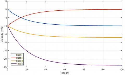
Figure 3. Simulation results for the four case-study scenarios

In this work, we will implement and test the continuous-time component representing a dynamic model of a vehicle using the model above, and dynamics are given that the vehicle's mass (m) is 1,000 kg. Gravitational acceleration (g) is 9.8 m/s^. The friction constant (k) is 50 [9]. We consider different modeling cases as given in Table 1. Also, Figure 3 shows the simulation results for the continuous-time component for the dynamic vehicle model using four different scenarios. The differences between the four cases can be generated by changing the values for F, θ, and v₀, as in Table 1. All four scenes tend to be constant in the end as they reach the peak/maximum possible velocity under the given parameters.

3.2 CTC for dynamic vehicle model with PID controller

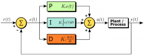
Indeed, the change of force due to road changes can be modeled using a customized PID controller (i.e., P, PI, or PD controller) [10]. PID controllers (P: proportional, I: integral, D: derivative) are commonly used in industrial control applications to regulate several process variables such as force, temperature, speed, and others] in the control loop feedback mechanism. Figure 4 illustrates the general block diagram of a PID controller [11] in a feedback loop where: r(t) is the desired process value, e (t) is the error value calculated continuously by the PID controller as the difference between a desired value (r(t)) and a measured process variable (y(t)), u(t) is the control variable determined by a weighted sum of the control terms (P, I, D) and y(t) is the measured process value.

4.png

Figure 4. Block diagram of PID controller

5.png

Figure 5. The modified vehicle models

In this work, we consider the implementation and simulation for the modified continuous-time component representing a dynamic model of a vehicle employing P/PI-Controllers [12, 13] to regulate the required force overtime using the model given in Figure 5 and the modified dynamics of Eq. (2).

To evaluate the provided model, we have used the following general parameters: The mass of the vehicle (m) is 1,000 kg, The gravitational acceleration (g) is 9.8 m/s², The friction constant (k) is 50 (dimensionless coefficient), The sample time (∆t) is 0.10 sec with total sampling time (t_s) of 120 sec, Desired velocity (or called reference point-R) is 10 m/s, Initial conditions (x(0), v(0))=(x_o, v₀)=(0m, 0m/s), The velocity error (e (t)) is calculated as e(t)=R-v(t). Also, the applied force F(t) to move the vehicle in an uphill direction is no longer assumed to be constant. Instead, we have modeled the variable force as a control variable by applying two different PID controller terms (i.e., P and PI) as follows:

Using P-Controller: For this case, we have only used the proportional term (P) of the PID controller with proportional parameter (K_p). Thus,

$F(t)=K_p \cdot e(t)$  → substitute this in Eq. (1), then:

$v(t+1)=v(t)+\frac{\Delta t\left(K_p . e(t)-k v(t)-m g \sin (\theta(t))\right)}{m}$                       (3)

where,

$\theta(t)=\left\{\right.$ Constant $\left(5^{\circ}\right.$ or $\left.10^{\circ}\right)$, Variable $\left.\left(\frac{1}{3} \sin (t / 5)\right)\right\}$

Using PI-Controller: For this case, we have used two terms of the PID controller: The proportional term (P) with proportional parameter (K_p) and the integral term (I) with integral parameter (K_I).

$F(t)=K_p \cdot e(t)+K_I \cdot \int_{t_i}^{t_{i+1}} e(t) \cdot d t$

→ substitute in Eq. (1), then:

$v(t+1)=v(t)+\frac{\Delta t\left(\begin{array}{c}K_p \cdot e(t)+K_I \cdot \int_{t_i}^{t_{i+1}} e(t) \cdot d t \\ -k v(t)-m g \sin \theta(t)\end{array}\right)}{m}$                      (4)

where,

$\theta(t)=\left\{\right.$ Constant $\left(5^{\circ}\right.$ or $\left.10^{\circ}\right)$, Variable $\left.\left(\frac{1}{3} \sin (t / 5)\right)\right\}$

For the integration part of model dynamics, we have calculated it numerically using the well-known Trapezoidal rule [14]. Finally, to get more insight, we consider several scenarios for vehicle velocity response, including:

$\bullet$ Vehicle Model with P-Controller:

$K_p=600, \theta=5^{\circ}=5 \frac{\pi}{180} \mathrm{rad}$

$\bullet$ Vehicle Model with P-Controller:

$K_p=600, \theta=10^{\circ}=10 \frac{\pi}{180} \mathrm{rad} \text {, }$

$\bullet$ Vehicle Model with PI-Controller:

$K_p=600, K_I=40, \theta=5 \frac{\pi}{180} \mathrm{rad} \text {, }$

$\bullet$ Vehicle Model with PI-Controller:

$K_p=600, K_I=40, \theta=10 \frac{\pi}{180} \mathrm{rad} \text {, }$

$\bullet$ Vehicle Model with P-Controller:

$K_p=600, \theta(t)=\frac{1}{3} \sin (t / 5) \mathrm{rad} \text {, }$

$\bullet$ Vehicle Model with PI-Controller:

$K_p=600, K_I=40, \theta(t)=\frac{1}{3} \sin (t / 5) \mathrm{rad}$

Besides, we have tried several experiments by tuning the different factors affecting the velocity response, such as the proportional gain $K_p$, integral gain $K_I$, the $\theta(t)$. For instance, Figure 6 shows the velocity response for the dynamic vehicle model using a $P$-controller with the following parameters: $K_p=600$ and $\theta=\left\{5^{\circ}, 10^{\circ}\right\}$. According to the figure, it can be seen that the $P$-controller with the prescribed setup parameters was not able to provide the required force to meet the desired velocity $(\mathrm{R}=10 \mathrm{~m} / \mathrm{s})$ for both cases of road grade $\left(5^{\circ}\right.$ or $\left.10^{\circ}\right)$. Another gain factor of the PID controller needs to be tuned up to enhance the force controllability, such as the integral gain $K_I$_.

6.png

Figure 6. The velocity of the vehicle in response to R=10 m/s and K_p=600

Figure 7 shows the velocity response for the dynamic vehicle model using the PI controller (after adding Integral gain I) with the following parameters: $K_p=600, K_I=40$ and $\theta=\left\{5^{\circ}, 10^{\circ}\right\}$. According to the figure, it can be seen that the PI-controller with the prescribed setup parameters has successfully provided the required force to meet the desired velocity (R=10 m/s) for both cases of road grade (5^o or 10^o) with a slightly faster response appeared for the road disturbance input signal of 10^o.

7.png

Figure 7. The velocity of the vehicle in response to $R=10 \mathrm{~m} / \mathrm{s}, K_p=$ 600, $K_I=$ 40

8.png

Figure 8. Velocity response: $R=10 \mathrm{~m} / \mathrm{s}, K_p=$ 600, $K_I=$ 40, $\theta(t)=\frac{1}{3} \sin \left(\frac{t}{5}\right) \mathrm{rad}$

9.png

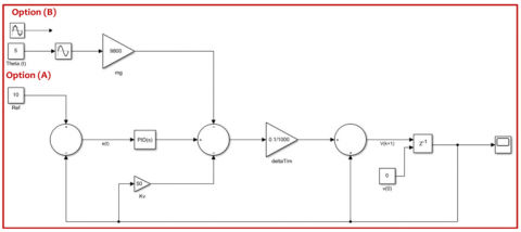
Figure 9. Simulink Implementation of Vehicle Model with P/PI controllers using two options: (A) $\theta(t)=5^{\circ}$ , $\theta(t)=10^{\circ}$ , (B) $\theta(t)=\frac{1}{3} \sin \left(\frac{t}{5}\right) \mathrm{rad}$

10.png

Figure 10. SimEvents model of the network node (transceiver node)

111.png

Figure 11. Simulink vehicle model with one networked PI-controller

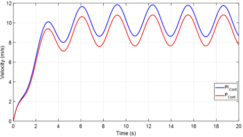
Figure 8 shows the response of the vehicle velocity for the dynamic vehicle model using a continuous-time disturbance input signal following a sinusoidal signal $\theta(t)=\frac{1}{3} \sin (t / 5) \mathrm{rad}$. Such a formula models the change in road condition as the vehicle driving on it. Besides, the figure considers the cruise controller using only a P-controller or PI-controller with the following parameters: $K_p=600, K_I=40$. According to the figure, it can be seen that the velocity response of such a vehicle motion dynamic follows a sinusoidal behavior. The vehicle motion velocity keeps fluctuating as a sinusoidal up and down between 7.5 m/s and 10.5 m/s for the cruise controller implementing the proportional gain (P) only. In contrast, it ranges from 8.5 m/s to 11.5 m/s for the cruise controller implementing the proportional and integral gains (PI). The results showed that the PI controller recorded more accurate results since the average range of its response approaches 10 m/s while the average response for the P controller approaches 9 m/s.

Moreover, according to the results mentioned above and discussions, we have observed a significant difference between the performance of P and PI controllers on the vehicle speed with superiority registered for the PI controller. Indeed, it would be more interested in acquiring the PI controller as it rapidly converges to the desired velocity [15]. Finally, recall the stateful continuous-time component model of how the speed of a vehicle changes because of the force applied to it by the engine [7] when the vehicle is moving on an uphill single-dimension graded road. In this model, we are controlling the force F(t) using the PID controller [11], mainly P & PI controllers. Finally, we are implementing the complete model using the Simulink toolbox [12], as given in Figure 9.

3.3 Cyber-physical dynamic vehicle model with PID controller

In this case, we are adding a cyber component that can control the physical system remotely through a communication network. Therefore, we have utilized the SimEvents  toolbox of Matlab to adopt the cyber part of the system by developing a network node model (transmit/receive) with the ability to simulate different random network time-delay. Recall the Simulink component models of the vehicle and cruise P-controller with vehicle dynamics as one block and the P-controller as another block and using the same parameters: $K_p=600, K_I=40$, constant disturbance θ(t)=10^o, variable disturbance $\theta(t)=\frac{1}{3} \sin \left(\frac{t}{5}\right) \mathrm{rad}$, and finally, the desired vehicle speed R= 10 m/s. The developed networking node is illustrated in Figure 10. The component considered the network uniform distribution in the timed-based random number distribution block with a minimum value of 0.01 and a maximum value of 0.1. The uniform distribution is meant to have evenly spaced time units starting at 0.01 to 0.1. the minimum and maximum values can be arbitrarily determined. The selected values (0.01 to 0.1) are more realistic for network nodes [0.01s, 0.1s].

To make use of the network as mentioned above the node, we have added one instance of the network node model to the vehicle-cruise controller using the Simulink model developed in Figure 9. The node has been inserted between the sensor and the controller only to end up with a vehicle model using a networked PI controller. The developed model of the vehicle with one networking node is illustrated in Figure 11. Note that θ(t) can be used as a constant $10^0$ (option A) or can be used as a variable disturbance using sinusoidal $\theta(t)=\frac{1}{3} \sin \left(\frac{t}{5}\right) \operatorname{rad}($ option $B)$.

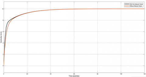
Accordingly, we have tested this model using different min-max values of the random distribution block and by using either constant disturbance $\theta(t)=10^0$ (10x(π/180) rad) or variable disturbance $\theta(t)=\frac{1}{3} \sin \left(\frac{t}{5}\right) \mathrm{rad}$. For instance, Figure 12 compares the velocity responses for the vehicle model with PI-controller on a graded road with fixed θ(t)=10⁰before and after adding a network node between the sensor and the controller. The network node employs a random number distribution block in this model to generate time delay values ∈ [0.01s, 0.1s] using a uniform random distribution. According to the figure, the vehicle response has been slightly delayed due to using a network node with the delay mentioned above boundaries.

12.png

Figure 12. Velocity response of vehicle model with and without incorporating one network node (θ=10⁰)

13.png

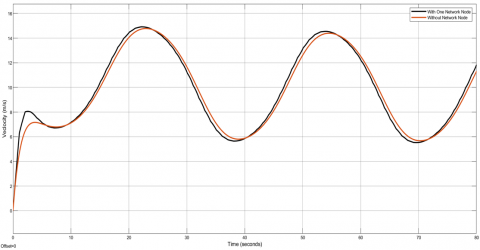
Figure 13. Velocity response of vehicle model with and without adding one network node ( $\theta(t)=\frac{1}{3} \sin \left(\frac{t}{5}\right) \mathrm{rad}$ )

Figure 13 illustrates the velocity responses for the vehicle model with PI controller on a graded road with variable sinusoidal disturbance $\theta(t)=\frac{1}{3} \sin \left(\frac{t}{5}\right) \mathrm{rad}$. The model considers two configurations: with and without adding a network node between the sensor and the controller. The main reason for adding the network node is to turn the system into a Cyber-Physical System. Without the network nodes (cyber part), the system is assumed to be a physical system node with no communication ability. Again, the network node uses a uniform random number distribution for time delay values ∈ [0.01s, 0.1s], and thus, the vehicle response has been slightly delayed due to the use of network node.

Moreover, to analyze the effect of network delay on the system, we have tested the vehicle velocity response with five different min-max values of the random distribution block. This includes: [0.01s, 0.1s], [0.05s, 0.1s], [0.1s, 1.0s], [0.5s, 2.0s] and [1.0s, 5.0s]. Almost the system was stable in all tests except for the last testing interval [1.0s, 5.0s] (largest delay range). The system showed unstable behavior under the same parameters and simulation time, as illustrated in Figure 14. Note that the system showed an unstable response in this random interval regardless of the disturbance of the road.

14.png

Figure 14. Velocity response of vehicle model with one network node using random delay time ∈ [1.0s, 5.0s]

15.png

Figure 15. Simulink vehicle model with two networked PI-controller

To enhance the system stability in response to the cyber control, we have added two instances of the network node model to the vehicle-cruise controller using the Simulink model developed in Figure 9. One has been inserted between the sensor and the controller and another node between the controller and the vehicle model to end up with a cyber-physical vehicle model using two networked PI-controller. The developed model of the vehicle model with two networking nodes is illustrated in Figure 15. the figure shows the variable disturbance block θ(t). Again, θ(t) can be used as a constant $10^0$  block.

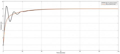
Similarly, we tested the velocity response for this model using different uniformly distributed random min-max values of the network nodes using $\theta(t)=\left\{\right.$ either $10^{\circ}$ or $\left.(1 / 3) \sin (t / 5) \mathrm{rad}\right\}$. Figure 16 compares the velocity responses for the vehicle model with PI-controller on a graded road with fixed $\theta(t)=10^{\circ}$ before and after adding two network nodes: one node was added between the sensor and the controller and another node between the controller and the vehicle model. In this test, we consider both network nodes to have a uniformly distributed time delay value ∈ [0.01s, 0.1s]. According to the figure, adding more network nodes resulted in an additional delay in the response signal, which spikes for the first couple of times.

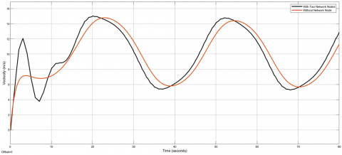
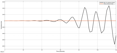
Figure 17 presents the velocity responses for the vehicle model with PI-controller of variable graded road θ(t)=(1/3)sin(t/5) rad considering two configurations: with and without adding two network nodes to the vehicle model. Besides, both network nodes employ a uniformly distributed time delay ∈ [0.01s, 0.1s]. As a result, the plot shows that adding more network nodes resulted in delaying the vehicle response following the delay values, with a signal spike appearing at the beginning of the response. Comparing the experimental results shown in Figure 13 and Figure 17, you can see that the cyber physical system incorporating one network node has a lower delay than one incorporating two nodes. Please focus on how the black curve in the case of one node (Figure 13) is more tightly coupled to the red curve (no network at all). At the same time, it has a larger delay in the case of two nodes (Figure 17).

16.png

Figure 16. Velocity response of vehicle model with and without incorporating two network nodes (θ=10⁰)

17.png

Figure 17. Velocity response of vehicle model with and without adding two network nodes $\left(\theta(t)=\frac{1}{3} \sin \left(\frac{t}{5}\right) \mathrm{rad}\right)$

18.png

Figure 18. Velocity response of vehicle model with two network nodes using random delay time ∈ [0.5s, 2.0s]

Finally, we have also performed five tests for the vehicle velocity in response to varying the min-max values of the random distribution block, including the intervals: [0.01s, 0.1s], [0.05s, 0.1s], [0.1s, 1.0s], [0.5s, 2.0s] and [1.0s, 5.0s]. As a result, the system showed stable behavior in the first three interval tests. However, under the same parameters and simulation time, the system becomes unstable at the distribution range of [0.5s, 2.0s] and [1.0s, 5.0s]. Figure 18 shows the velocity response for the vehicle model employing the distribution range of [0.5s, 2.0s] regardless of the disturbance of the road.