Sangeetha Sekar* | Sivakami Lakshmi Nathan | Lakshmi Priya Saravanathan
© 2022 IIETA. This article is published by IIETA and is licensed under the CC BY 4.0 license (http://creativecommons.org/licenses/by/4.0/).
OPEN ACCESS
The effect of velocity slip with viscosity variation between porous rough circular stepped plates with couple stress fluid is examined. A stochastic random variable having a non-zero mean, variance, and skewness is used to model a more general type of surface roughness equation also the modified Reynolds equation accounting for pressure dependent viscosity is analytically derived. The numerical solution obtained for the non-dimensionless pressure, load carrying capacity and time. It is observed that the impact of roughness and viscosity variation using a couple stress fluid between circular stepped plates has been discussed. These effects improved the ability of load carrying capacity as compared to the corresponding Newtonian case.
viscosity variation, couple stress fluid, velocity slip, surface roughness, porous
The surfaces have been assumed to be smooth in the majority of theoretical analysis of hydrodynamic lubrication. This is an unrealistic assumption for the bearings operation with small film thickness. The Stochastic theory of surface roughness introduced by Christensen [1]. For various geometries the stokes couple stress theory has been used to study behaviour of couple stress fluid [2, 3]. The effect of couple stress fluid between circular stepped plates is studied by Naduvinamani and Siddangouda [4] and observed that the presence of couple stress fluid increases the load carrying capacity. Naduvinamani and Siddangouda [5] found that the influence of porous using couple stress fluid improves the squeezing characteristics. The analysis of squeeze film lubrication using couple stress fluid with viscosity variation plays an important role. Previous concepts have been based on the assumption of constant viscosity, even though it is both a function of both pressure and temperature. In many real-world applications, the viscosity variation with temperature is essential. Barus analysis the interaction between the viscosity variation and pressure [6] is given by relation $\mu=\mu_o e^{\beta p}$.
Hanumagowda et al. [7] examined the impact on circular stepped plates with viscosity variation using micropolar fluid. They showed that by the presence of viscosity variation pressure increases. The influence of viscosity variation between the circular stepped plates using couple stress fluid is examined by Hanumagowda [8] and found that the pressure and load carrying capacity is enhanced with an increase in viscosity variation parameter. Sangeetha and Govindarajan [9] analyzed the effects of magneto hydrodynamic(mhd) and viscosity variation using couple stress fluid between circular stepped plates. It is observed that the combined influence of couple stress and magnetic effects are significant. The results indicated that viscosity variation with couple stress was better than Newtonian fluid and the performance squeeze film characteristic enhanced. Sangeetha and Kesavan [10] examined the effect of velocity slip and viscosity variation between triangular plates using couple stress fluid. It is noted that when a fluid flow around a porous medium of very small permeability, a zero tangential velocity at the permeable interface is assumed. As the flow within the porous medium becomes significant, this condition turns out to be inaccurate as shown for instance by the experiments performed by Beavers and Joseph [11]. These experiments established the validity of the slip boundary condition at the interface between the porous medium and the clear fluid qualitatively.
Henceforth no investigation has been carried out to examine the viscosity variation with velocity slip so the present study deals with the viscosity variation and velocity slip between rough porous circular stepped plates using couple stress fluid.
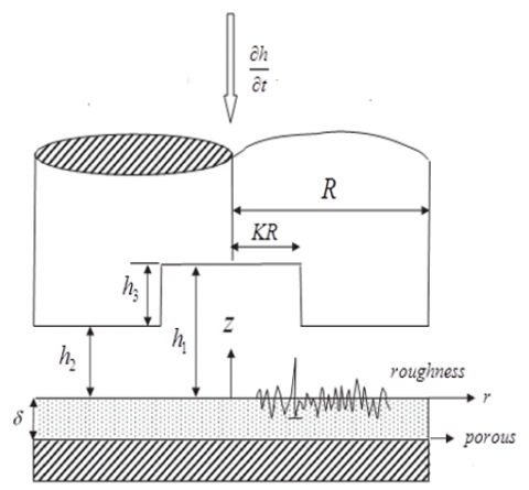
Figure 1. Configuration of the circular stepped plates
Figure 1 demonstrates the configuration of circular stepped plates. The top plate approaches the other, which is rough porous surface in nature with constant velocity. The bottom plate is stationary. The couple stress fluid is considered as the lubricant in the film region. The Beavers-Joseph approximation [11] is used for studying hydrodynamic lubrication for velocity slip at the porous interface.
$\mu \frac{\partial^2 u}{\partial z^2}-\eta \frac{\partial^4 u}{\partial z^4}=\frac{\partial p}{\partial r}$ (1)
$\frac{\partial p}{\partial z}=0$ (2)
$\frac{1}{r} \frac{\partial}{\partial r}(r u)+\frac{\partial w}{\partial z}=0$ (3)
The modified Darcy's law governs the flow of a couple stress fluid in a porous region which takes into account polar effects by using Naduvinamani [11].
$u^*=\frac{-k}{\mu(1-\beta)} \frac{\partial p^*}{\partial x^*}$ (4)
$v^*=\frac{-k}{\mu(1-\beta)} \frac{\partial p^*}{\partial y^*}$ (5)
$\frac{\partial u^*}{\partial x}+\frac{\partial v^*}{\partial y}=0$ (6)
The boundary conditions are at z = 0.
$\frac{\alpha}{\sqrt{k}}\left(u-u^*\right)=\frac{\partial u}{\partial z}$
$w=w^*, \frac{\partial^2 u}{\partial z^2}=0$ (7)
The boundary conditions are at z=h.
$u=0, \frac{\partial^2 u}{\partial z^2}=0, w=\frac{\partial h}{\partial t}$ (8)
The solution of Eq. (1) subject to the boundary conditions (7) and (8) is obtained in the form
$u=\frac{1}{2 \mu_o e^{\beta p}} \frac{\partial p}{\partial r}\left\{\begin{array}{r}(z-h)\left[z+\frac{1}{3} h \xi_1-2 \xi_2 l \tanh \left(\frac{h}{2 l}\right)\right] \\ +2 l^2\left[1-\frac{\cosh \frac{(2 z-h) / 2 l}{2 l}}{\cosh \left(\frac{h}{2 l}\right)}\right]\end{array}\right\}$ (9)
where, $\xi_1=\frac{3\left[2 s^2 \alpha^2+(1-\beta) s h\right]}{h(h+s)(1-\beta)}, \xi_2=\frac{s}{h+s}$.
The pressure satisfies the Laplace equation $\nabla^2 p^*=0$ in the porous medium. The modified Reynolds type equation for the pressure is obtained by substituting the Eq. (9) in Eq. (3) and then integrating and also using the condition (7) and (8) we get.
$\frac{\partial}{\partial r}\left\{\left[f\left(h, \xi_1, \xi_2, l\right) e^{-\beta p}+\frac{12 k \delta}{(1-\beta)}\right] r \frac{\partial p}{\partial r}\right\}=12 r \frac{\partial h}{\partial t}$ (10)
where,
$f\left(h, \xi_1, \xi_2, l\right)=h^3\left(1+\xi_1\right)-6 h^2 l \xi_2 \tanh \left(\frac{h}{2 l}\right)-12 l^2\left(h-2 \tanh \left(\frac{h}{2 l}\right)\right)$
The volume flux of the lubricant is given by
$Q=2 \pi r \int_0^h u d z$ (11)
$Q=-\frac{\pi r e^{-\beta p}}{6 \mu_o} \frac{\partial p}{\partial r} f\left(h, \xi_1, \xi_2, l\right)$ (12)
To represent the surface roughness proposed by Christensen [1], the mathematical expression for the film thickness is considered to be consisting of two parts $H=h(t)+h_s(x, y, \xi)$. where h(t) is the height of the nominal smooth part of the fluid film region, and $h_s(x, y, \xi)$ is the part due to the surface asperities measured from the nominal level and is a randomly varying quantity of zero mean, and ξ is the index parameter determining a definite roughness structure. Further, stochastic part hs is considered to have the probability density function f(hs) defined over the domain (-c≤hs≤c) Where c is the maximum deviation from the mean film thickness.
For the longitudinal one-dimensional roughness, the film thickness assumes the form using Naduvinamani and Siddangouda [12] H=h(t)+ hs(x, ξ).
$f\left(h_s\right)=\left\{\begin{array}{cc}\frac{35}{32 c^7}\left(c^2-h_s^2\right)^3 & -c \leq h_s \leq c \\ 0 & \text { elsewhere }\end{array}\right.$ (13)
where, $\bar{\sigma}=\frac{c}{3}$ is the standard deviation
$\alpha^*=E\left(h_s\right)$ (14)
$\sigma^*=E\left[\left(h_s-\alpha^*\right)^2\right]$ (15)
$\varepsilon^*=E\left[\left(h_s-\alpha^*\right)^3\right]$ (16)
$E(.)=\int_{-\infty}^{\infty}(.) f\left(h_s\right) d h_s$ (17)
In Eqns. (10) and (12) the dimensionless form is obtained as
$\frac{\partial}{\partial r^*}\left\{e^{-G p^*} F\left(H^*, \xi_1, \xi_2, l^*, \alpha^*, \varepsilon^*, \sigma^*, \psi\right) r^* \frac{\partial p^*}{\partial r^*}\right\}=-12 r^*$ (18)
Using the non- dimensional quantities
$Q^*=\frac{\pi r^* e^{-G p^*}}{6} \frac{\partial p^*}{\partial r^*} F\left(H^*, \xi_1, \xi_2, l^*, \alpha^*, \varepsilon^*, \sigma^*, \psi\right)$ (19)
$H_2^*=\frac{h_2}{h_o}, H_3^*=\frac{h_3}{h_o}, l^*=\frac{l}{h_o}, r^*=\frac{r}{h_o}, Q^*=\frac{Q \mu_o R^2}{h_2^3}, G=$
$\frac{\beta \mu_o R^2\left(-\frac{\partial h}{\partial t}\right)}{h_2^3}, p^*=\frac{p h_2^3}{R^2 \mu_o\left(\frac{-\partial h}{\partial t}\right)}, \psi=\frac{k \delta}{h_2^3}, s=\frac{\sigma^*}{h_2}, \sigma^*=\frac{\sqrt{k}}{\alpha}$
$H^*=\frac{h}{h_2}$
$F\left(H^*, \xi_1, \xi_2, l^*, \alpha^*, \varepsilon^*, \sigma^*, \psi\right)=\left(1+\xi_1\right) g_1-6 l^* H^{2 *} \xi_2 g_2 g_3-12^* l^2\left(H+\alpha^*\right)+g_4+\frac{12 \psi}{1-\beta}$
$g_1=H^{* 3}+3 H^{* 2} \alpha^*+3 H^*\left(\sigma^{* 2}+\alpha^{* 2}\right)+\varepsilon^*+3 \alpha^* \sigma^{* 2}+\alpha^{* 3}$
$g_2=H^{* 2}+\sigma^{* 2}+\alpha^{* 2}+2 H^* \alpha^*$
$g_3=\tanh \left(\frac{H^*}{l^*}\right)+\left(1-\tanh ^2\left(\frac{H^*}{2 l}\right)\right) \frac{1}{24 l^3}\left(12 l^2 \alpha^*-\varepsilon^*-3 \alpha^* \sigma^{* 2}-\alpha^{* 3}\right)$
$g_4=24 l^3 \tanh \left(\frac{H^*}{l^*}\right)+\left(1-\tanh ^2\left(\frac{H^*}{2 l}\right)\right)\left(12 l^2 \alpha^*-\varepsilon^*-3 \alpha^* \sigma^{* 2}-\alpha^{* 3}\right)$
Reynolds equation in region I: (0≤r*≤K)
$\frac{\partial}{\partial r^*}\left\{e^{-G p_1^*} F^*\left(H^*, \xi_{11}, \xi_{12}, l^*, \alpha^*, \varepsilon^*, \sigma^*, \psi\right) r^* \frac{\partial p^*}{\partial r^*}\right\}=-12 r^*$ (20)
Reynolds equation in region II: (K≤r*≤1)
$\frac{\partial}{\partial r^*}\left\{e^{-G r_2^*} F^*\left(\xi_{21}, \xi_{22}, l^*, \alpha^*, \varepsilon^*, \sigma^*, \psi\right) r^* \frac{\partial p^*}{\partial r^*}\right\}=-12 r^*$ (21)
The pressure boundary conditions are
$\frac{d p_1^*}{d r^*}=0$ at $r^*=0$ (22)
$p_2^*=0$ at $r^*=1$ (23)
$p_1^*=p_2^*$ at $r^*=R$ (24)
$Q_1^*=Q_2^*$ at $r^*=R$ (25)
The solution of Eqns. (20) and (21) satisfying the conditions (22), (23), (24) and (25) is of the form.
Pressure in region I: P1*=(0≤r*≤K)
$p_1^*=-\frac{1}{G} \ln \left\{\left(\begin{array}{l}\frac{3 G\left(r^{* 2}-K^2\right)}{F_1^*\left(H_1^*, \xi_{11}, \xi_{12}, l^*, \alpha^*, \varepsilon^*, \sigma^*, \psi\right)} \\ \frac{3 G\left(K^2-1\right)}{F_2^*\left(\xi_{21}, \xi_{22}, l^*, \alpha^*, \varepsilon^*, \sigma^*, \psi\right)}\end{array}\right)+1\right\}$ (26)
Pressure in region II: P2*=(K≤r*≤1)
$p_2^*=-\frac{1}{G} \ln \left\{\frac{3 G\left(r^{* 2}-1\right)}{F_2^*\left(\xi_{21}, \xi_{22}, l^*, \alpha^*, \varepsilon^*, \sigma^*, \psi\right)}+1\right\}$ (27)
where,
$F_1\left(H_1^*, \xi_{11}, \xi_{12}, l^*, \alpha^*, \varepsilon^*, \sigma^*, \psi\right)=\left(1+\xi_{11}\right) g_{11}-6 l^* \xi_{12} g_{12} g_{13}-12^* l^2\left(H_1^*+\alpha^*\right)+g_{14}+\frac{12 \psi}{1-\beta}$
$g_{11}=H_1^{* 3}+3 H_1^{* 2} \alpha^*+3 H_1^*\left(\sigma^{* 2}+\alpha^{* 2}\right)+\varepsilon^*+3 \alpha^* \sigma^{* 2}+\alpha^{* 3}$
$g_{12}=H_1^{* 2}+\sigma^{* 2}+\alpha^{* 2}+2 H_1^* \alpha^*$
$g_{13}=\tanh \left(\frac{H_1^*}{l^*}\right)+\left(1-\tanh ^2\left(\frac{H_1^*}{2 l}\right)\right) \frac{1}{24 l^3}\left(12 l^2 \alpha^*-\varepsilon^*-3 \alpha^* \sigma^{* 2}-\alpha^{* 3}\right)$
$g_{14}=24 l^3 \tanh \left(\frac{H_1^*}{l^*}\right)+\left(1-\tanh ^2\left(\frac{H_1^*}{2 l}\right)\right)\left(12 l^2 \alpha^*-\varepsilon^*-3 \alpha^* \sigma^{* 2}-\alpha^{* 3}\right)$
$\xi_{11}=\frac{3\left[2 s^2 \alpha^2+(1-\beta) s H_1^*\right]}{H_1^*\left(H_1^*+s\right)(1-\beta)}, \xi_{12}=\frac{s}{H_1^*+s}$
$F_2^*\left(\xi_{21}, \xi_{22}, l^*, \alpha^*, \varepsilon^*, \sigma^*, \psi\right)=\left(1+\xi_{21}\right) g_{21}-6 l^* \xi_{22} g_{22} g_{23}-12^* l^2\left(1+\alpha^*\right)+g_{24}+\frac{12 \psi}{1-\beta}$
$g_{21}=1+3 \alpha^*+3\left(\sigma^{* 2}+\alpha^{* 2}\right)+\varepsilon^*+3 \alpha^* \sigma^{* 2}+\alpha^{* 3}$
$g_{22}=1+\sigma^{* 2}+\alpha^{* 2}+2 \alpha^*$
$g_{23}=\tanh \left(\frac{1}{l^*}\right)+\left(1-\tanh ^2\left(\frac{1}{2 l}\right)\right) \frac{1}{24 l^3}\left(12 l^2 \alpha^*-\varepsilon^*-3 \alpha^* \sigma^{* 2}-\alpha^{* 3}\right)$
$g_{24}=24 l^3 \tanh \left(\frac{1}{l^*}\right)+\left(1-\tanh ^2\left(\frac{1}{2 l}\right)\right)\left(12 l^2 \alpha^*-\varepsilon^*-3 \alpha^* \sigma^{* 2}-\alpha^{* 3}\right)$
$\xi_{21}=\frac{3\left[2 s^2 \alpha^2+(1-\beta) s\right]}{1(1+s)(1-\beta)}, \quad \xi_{22}=\frac{s}{1+s}$
Substituting the expression of the film pressure and integrating the Eqns. (26) and (27). we can obtain the load carrying capacity w is obtained in the form
$w=2 \pi \int_0^{K R} r p_1 d r+2 \pi \int_{K R}^1 r p_2 d r$ (28)
The load carrying capacity equation in dimensionless form is acquired as
$
w^*=\left\{\frac{w h_2^3}{\mu_0 R^4\left(\frac{-d h}{d t}\right)}\right\}=-\frac{2 \pi}{G} \int_0^K \ln \left\{\left(\begin{array}{c}
\frac{3 G\left(r^{* 2}-K^2\right)}{F_1^*\left(H_1^*, \xi_{11}, \xi_{12}, l^*, \alpha^*, \varepsilon^*, \sigma^*, \psi\right)}+ \\
\frac{3 G\left(K^2-1\right)}{F_2^*\left(\xi_{21}, \xi_{22}, l^*, \alpha^*, \varepsilon^*, \sigma^*, \psi\right)}
\end{array}\right)+1\right\} r^* d r^*-\frac{2 \pi}{G} \int_K^1 \ln \left\{\frac{3 G\left(r^{* 2}-1\right)}{F_2^*\left(\xi_{21}, \xi_{22}, l^*, \alpha^*, \varepsilon^*, \sigma^*\right)}+1\right\} r^* d r^*
$ (29)
The time height relationship in dimensionless form
$T^*=\left\{\frac{w t h_0^2}{\mu_0 R^4}\right\}-\frac{2 \pi}{G} \int_{h_f}^1 \int_0^K \ln \left\{\left(\begin{array}{c}\frac{3 G\left(r^{* 2}-K^2\right)}{F_1^*\left(H_2^*, H_3^*, \xi_{31}, \xi_{32}, l^*, \alpha^*, \varepsilon^*, \sigma^*, \psi\right)} \\ \frac{3 G\left(K^2-1\right)}{F_2^*\left(H_2^*, \xi_{41}, \xi_{42}, l^*, \alpha^*, \varepsilon^*, \sigma^*, \psi\right)}\end{array}\right)+1\right\} r^* d r^* d h_2^*-\frac{2 \pi}{G} \int_{h_f}^1 \int_K^1 \ln \left\{\left(\frac{3 G\left(r^{* 2}-1\right)}{F_2^*\left(H_2^*, \xi_{41}, \xi_{42}, l^*, \alpha^*, \varepsilon^*, \sigma^*, \psi\right)}\right)+1\right\}$ (30)
where,
$F_1^*\left(H_2^*, H_3^*, \xi_{31}, \xi_{32}, l^*, \alpha^*, \varepsilon^*, \sigma^*, \psi\right)=\left(1+\xi_{31}\right) g_1-6 l^* \xi_{32} g_{32} g_{33}-12^* l^2\left(H_2^*+H_3^*+\alpha^*\right)+g_{34}+\frac{12 \psi}{1-\beta}$
$g_{31}=\left(H_2^*+H_3^*\right)^3+3\left(H_2^*+H_3^*\right)^2 \alpha^*+3\left(H_2^*+H_3^*\right)\left(\sigma^{* 2}+\alpha^{* 2}\right)+\varepsilon^*+3 \alpha^* \sigma^{* 2}+\alpha^{* 3}$
$g_{32}=\left(H_2^*+H_3^*\right)^2+\sigma^{* 2}+\alpha^{* 2}+2\left(H_2^*+H_3^*\right) \alpha^*$
$g_{33}=\tanh \left(\frac{H_2^*+H_3^*}{l^*}\right)+\left(1-\tanh ^2\left(\frac{H_2^*+H_3^*}{2 l}\right)\right) \frac{1}{24 l^3}\left(12 l^2 \alpha^*-\varepsilon^*-3 \alpha^* \sigma^{* 2}-\alpha^{* 3}\right)$
$g_{34}=24 l^3 \tanh \left(\frac{H_2^*+H_3^*}{l^*}\right)+\left(1-\tanh ^2\left(\frac{H_2^*+H_3^*}{2 l}\right)\right)\left(12 l^2 \alpha^*-\varepsilon^*-3 \alpha^* \sigma^* 2-\alpha^*\right)$
$\xi_{31}=\frac{3\left[2 s^2 \alpha^2+(1-\beta) s\left(H_2^*+H_3^*\right)\right]}{\left(H_2^*+H_3^*\right)\left(H_2^*+H_3^*+s\right)(1-\beta)}, \xi_{32}=\frac{s}{H_2^*+H_3^*+s}$
$F_2^*\left(H_2^*, \xi_{41}, \xi_{42}, l^*, \alpha^*, \varepsilon^*, \sigma^*, \psi\right)=\left(1+\xi_{41}\right) g_{41}-6 l^* \xi_{42} g_{42} g_{43}-12^* l^2\left(H_2^*+\alpha^*\right)+g_{44}+\frac{12 \psi}{1-\beta}$
$g_{41}=H_2^{* 3}+3 H^{* 2} \alpha^*+3 H_2^*\left(\sigma^{* 2}+\alpha^{* 2}\right)+\varepsilon^*+3 \alpha^* \sigma^{* 2}+\alpha^{* 3}$
$g_{42}=H_2^{* 2}+\sigma^{* 2}+\alpha^{* 2}+2 H_2^* \alpha^*$
$g_{43}=\tanh \left(\frac{H_2^*}{l^*}\right)+\left(1-\tanh ^2\left(\frac{H_2^*}{2 l}\right)\right) \frac{1}{24 l^3}\left(12 l^2 \alpha^*-\varepsilon^*-3 \alpha^* \sigma^{* 2}-\alpha^{* 3}\right)$
$g_{44}=24 l^3 \tanh \left(\frac{H_2^*}{l^*}\right)+\left(1-\tanh ^2\left(\frac{H_2^*}{2 l}\right)\right)\left(12 l^2 \alpha^*-\varepsilon^*-3 \alpha^* \sigma^{* 2}-\alpha^{* 3}\right)$
$\xi_{41}=\frac{3\left[2 s^2 \alpha^2+s(1-\beta) H_2^*\right]}{H_2^*\left(H_2^*+s\right)(1-\beta)}, \xi_{42}=\frac{s}{H_2^*+s}$
To understand the effect of various parameters involved in this problem, a graphical illustration of slip parameter s, viscosity variation parameter G, couple stress parameter l*, permeability parameter ψ, a measure of the symmetry of the stochastic random variable ε*, the standard deviation of the film thickness σ*, mean of the stochastic film thickness α* are presented. The following ranges of the values for these parameters are used in the numerical computations of the results. α*, ε*=-0.1, -0.05, 0.05, 0.1; l*=-0.1, 0.2, 0.3, 0.4; σ*=-0.1, 0.2, 0.3, 0.4; ψ=0.01, 0.02, 0.03, 0.04; G=0.01-0.04. The range of the parameter considered from the Hanumagowda et al. [7] and Naduvinamani et al. [13].
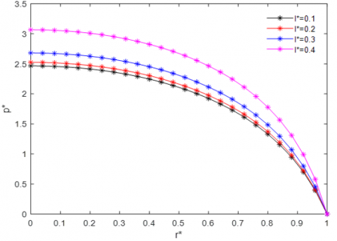
Figure 2 shows the variation of pressure p* as a function of r* for different values of couple stress parameter l*. Pressure rises, when the function of l*takes different values. The couple stress act as an added force in the fluid. This force is one of the factors that contribute to an increase in pressure.
Figure 2. Variation with r* for different values of couple stress parameter l* on dimensionless pressure p* with α*=0.05, σ*=0.2, ψ=0.01, H*=0.1, ε*=0.01, β=0.3, G=0.01, s=0.1
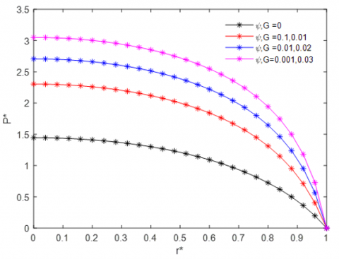
Figure 3 shows the variation of pressure p* as a function of r* for different values of viscosity variation parameter G. The results indicate that as the viscosity variation parameter increases the pressure increases. Since viscosity is the fluid’s resistance to motion, there is a greater force needed to maintain the mass continuity of the fluid. As expected, the force increases the pressure increases.
Figure 3. Variation with r* for different values of viscosity variation parameter G on dimensionless pressure p* with α*=0.05, σ*=0.3, ψ=0.01, H*=0.4, ε*=0.01, β=0.3, l*=0.2, s=0.1
Figure 4 shows the variation of pressure p* as a function of r* for different values of viscosity variation parameter $\psi$ and permeability parameter ψ. when (ψ, G=0) the equation reduces to solid case and non iso- viscous case. $f(h, l)=h^3-12 l^2+24 l^3 \tanh \left(\frac{h}{2 l}\right)$. The limiting case of f(h, l) reduces to the results of Naduvinamani and Siddangouda [4]. It is found that the viscosity variation is more prominent for pressure relative to the non iso -viscous case.
Figure 4. Variation with r* for different values of ψ and viscosity variation parameter G on dimensionless pressure p* with α*=0.02, σ*=0.3, H*=0.2, ε*=0.01, β=0.3, l*=0.2, s=0.1
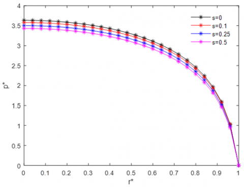
Figure 5. Variation with r* for different values of velocity slip parameter S on dimensionless pressure p* with α*=0.02, σ*=0.3, G=0.01, H*=0.2, ε*=0.01, β=0.3, l*=0.2, ψ=0.1
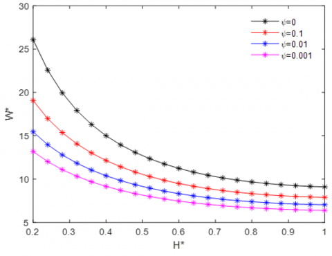
Figure 6. Variation with height H* for different values of permeability parameter ψon load carrying capacity w* with α*=0.05, σ*=0.2, β=0.3, l*=0.4, s=0.25, ε*=0.01, G=0.01
Figure 5 shows the variation of pressure p* as a function of r* for different values of velocity slip parameter S. The pressure p* decreases for increasing values of slip parameter.
Figure 6 shows the variation of load carrying capacity $w^*$ as a function of H* for different values permeability parameter ψ. It is demonstrated that the load carrying capacity also increases as the permeability parameter value ψ increases.
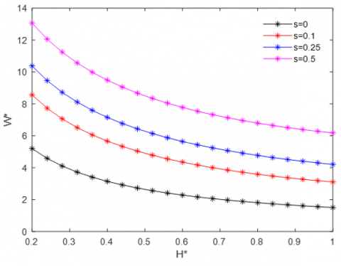
Figure 7. Variation with height H* for different values of slip parameter S on load carrying capacity w* with α*=0.05, σ*=0.2, β=0.3, l*=0.4, ψ=0.01, ε*=0.01, G=0.01
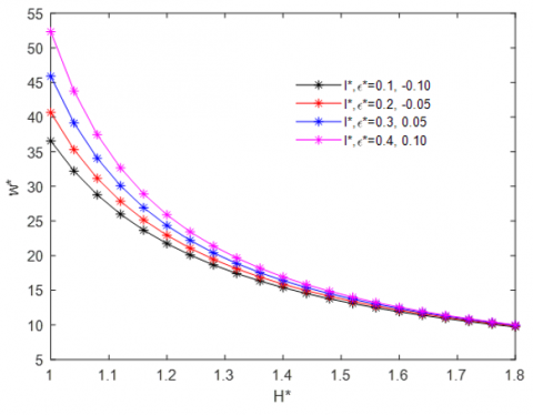
Figure 8. Variation with height H* for different parameter values of couple stress l* and measure of the symmetry of the stochastic random variable ε* on load carrying capacity w* with α*=0.05, σ*=0.2, β=0.3, ψ=0.01, G=0.01
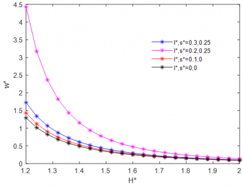
Figure 9. Variation with height H* for different parameter values of couple stress l*and slip parameter S on load carrying capacity w* with α*=0.05, σ*=0.2, β=0.3, ψ=0.01, G=0.01, ε*=0.01
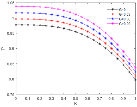
Figure 10. Variation with time T* for different values viscosity variation parameter G on K with α*=0.05, σ*=0.2, β=0.3, l*=0.4, ψ=0.01, ε*=0.01, hf=0.6, h3=0.15
Figure 7 shows the variation of load carrying capacity w* as a function of H* for different values of slip parameter S. It is well known that the load carrying capacity increases with the slip parameter value. Also, viscosity variation parameter enhances the load carrying capacity of the circular stepped plates.
Figure 8 shows variation with height for different parameter values of couple stress l* and measure of the symmetry of the stochastic random variable ε* on load carrying capacity w*. A standardized pattern of roughness is considered. Results demonstrate that the negatively skewed pattern of roughness improves the efficiency of time and load carrying. Furthermore, relative to the standard non-conducting lubricant instance, the viscosity variation with velocity slip characterized by the slip parameter improves the efficiency of the lubrication.
Figure 9 describes variation with height H* with load carrying capacity w* for different parameter values of couple stress l* and slip parameter s. When (l*, s=0) the present investigation reduces to Newtonian and non-porous case studied by Hamrock et al. [14] results F*=H*3. It is noted that the slip parameter and couple stress fluid enhance the load carrying capacity. This is because as the couple stress fluid offers more resistance to the moving fluid, the large amount of fluid would remain in the region.
Figure 10 shows the variation of time T* as a function of K for different values of viscosity variation parameter G. The presence of couple stress fluid is responsible to strengthen the response time as compared with non-isoviscous scenario.
On the whole, the viscosity variation produces an enhancement in the load carrying capacity and the response time as compared to the non-isoviscous case [15-17].
In this paper viscosity variation with couple stress fluid between circular stepped plates is studied. From the numerical results, the following conclusions can be drawn.
• The Reynolds equation using couple stress fluid is obtained by taking viscosity variation along with the film thickness into consideration. The expressions for pressure, load carrying capacity and time are obtained.
•The effect of permeability is to decrease the load carrying capacity as the height increases, whereas for increasing slip parameter the load carrying capacity increases. The obvious reason for this happens is that larger values lead to a greater number of voids on the porous facing, allowing the fluid to percolate into a porous region. Thus, pores on the porous facing become the main path for fluid to flow.
• The surface roughness and couple stress fluid promote the pressure distribution in the fluid region. This is because as the couple stress fluid offers more resistance to the moving fluid, the larger amount of fluid would remain in the region. On the other hand, the roughness asperities present on the bearing surface also reduce the velocity of the fluid. Furthermore, the amount of leakage of the lubricant along the sidewise direction is again reduce by the presence of the surface asperities.
• The influence of viscosity variation with couple stress fluid as lubricant lead to the increase in response time. The influence of a higher value of the viscosity variation parameter provides a significantly greater change in the response time. This behavior is due to the higher film pressure generated by the higher value of couple stress fluid.
By the above analyses, it is found that the pressure decreases for increasing value of the viscosity variation parameter. Also, it is observed that the squeeze is slower in couple stress fluid. The time of approach T increases, indicates that couple stress fluid are better lubricant.
The following data are considered for the squeeze film between circular stepped plates with non-Newtonian couple stress fluid:
Radius: R=10mm
Minimum film thickness: h2=0.5mm
Maximum film thickness: h2=0.5-0.1,0.11,0.12,0.13mm
Viscosity: μ=500cp
Material constant characterizing couple stress parameter: η=1.25×10⁻¹⁵Ns, 5×10-11Ns, 11.25×10⁻¹⁵Ns.
|
G |
Viscosity parameter |
|
E |
Expectancy operator |
|
h |
Film thickness=(h+hs) |
|
H* |
Non-dimensional film thickness=$\left(\frac{h}{h_0}\right)$ |
|
l |
Couple stress parameter =$\left(\frac{\eta}{\mu}\right)^{\frac{1}{2}}$ |
|
l* |
Non-dimensional couple stress parameter |
|
Greek symbols |
|
|
$\alpha$ |
Mean of the stochastic film thickness |
|
$\beta$ |
Coefficient of pressure-dependent viscosity |
|
$\delta$ |
Porous layer thickness |
|
$\sigma$ |
Standard deviation of the film thickness |
|
$\sigma^2$ |
Variance |
|
$\beta$ |
Percolation parameter = $\frac{\eta}{\mu k}$ |
|
$\eta$ |
Material constant characterizing couple stress |
|
$\psi$ |
Permeability parameter = $\frac{k \delta}{h_0^3}$ |
|
µ |
Viscosity co-efficient |
[1] Christensen, H. (1969). Stochastic models for hydrodynamic lubrication of rough surfaces. Proceedings of the Institution of Mechanical Engineers, 184(1): 1013-1026. https:/doi.org/10.1243/PIME_PROC_1969_184_074_02
[2] Sujatha, E., Kesavan, S. (2017). Performance of a porous parallel elliptic plates lubricated with couple stress fluids considering the effect of slip velocity and viscosity variation. ARPN Journal of Engineering and Applied Sciences, 12(6): 1835-1843.
[3] Naduvinamani, N.B., Fathima, S.T., Hanumagowda, B.N. (2011). Magneto-hydrodynamic couple stress squeeze film lubrication of circular stepped plates. Proceedings of the Institution of Mechanical Engineers, Part J: Journal of Engineering Tribology, 225(3): 111-119. https:/doi.org/10.1177/1350650110397460
[4] Naduvinamani, N.B., Siddangouda, A. (2009). Squeeze film lubrication between circular stepped plates of couple stress fluids. Journal of the Brazilian Society of Mechanical Sciences and Engineering, 31: 21-26. https://doi.org/10.1590/S1678-58782009000100004
[5] Naduvinamani, N.B., Siddangouda, A. (2007). Combined effects of surface roughness and couple stresses on squeeze film lubrication between porous circular stepped plates. Proceedings of the Institution of Mechanical Engineers, Part J: Journal of Engineering Tribology, 221(4): 525-534. https://doi.org/10.1243/13506501JET 204
[6] Barus, C. (1893). ART. X.--Isothermals, Isopiestics and Isometrics relative to Viscosity. American Journal of Science (1880-1910), 45(266): 87-96. https://doi.org/10.2475/ajs.s3-45.266.87
[7] Hanumagowda, B.N., Shivakumar, H.M., Raju, B.T., Kumar, J.S. (2016). Combined Effect of Pressure-Dependent Viscosity and Micropolar Fluids on Squeeze Film Circular Stepped Plates. International Journal of Mathematics Trends and Technology, 37(3): 175-183. https://doi.org/10.14445/22315373/IJMTT-V37P523
[8] Hanumagowda, B.N., Raju, B.T., Kumar, J.S., Vasanth, K.R. (2018). Effect of pressure dependent viscosity on couple stress squeeze film lubrication between porous circular stepped plates. In Journal of Physics: Conference Series, 1000(1): 012081. https://doi.org/10.1088/1742-6596/1000/1/012081
[9] Sangeetha, S., Govindarajan, A. (2019). Analysis of viscosity variation with MHD on circular stepped plates in couple stress fluid. Journal of Interdisciplinary Mathematics, 22(6): 889-901. https://doi.org/10.1080/09720502.2019.1688945
[10] Sangeetha, S., Kesavan, S. (2019). Effect of load carrying capacity and pressure distribution with viscosity variation and velocity slip using couple stress fluid for porous triangular plates with MHD. In AIP Conference Proceedings, 2112(1): 020168. https://doi.org/10.1063/1.5112353
[11] Beavers, G.S., Joseph, D.D. (1967). Boundary conditions at a naturally permeable wall. Journal of Fluid Mechanics, 30(1): 197-207. https://doi.org/10.1017/S0022112067001375
[12] Naduvinamani, N.B., Siddangouda, A. (2007). Effect of surface roughness on the hydrodynamic lubrication of porous step-slider bearings with couple stress fluids. Tribology International, 40(5): 780-793. https://doi.org/10.1016/j.t riboint.2006.07.003
[13] Naduvinamani, N.B., Fathima, S.T., Hiremath, P.S. (2004). On the squeeze effect of lubricants with additives between rough porous rectangular plates. ZAMM-Journal of Applied Mathematics and Mechanics/Zeitschrift für Angewandte Mathematik und Mechanik: Applied Mathematics and Mechanics, 84(12): 825-834. https://doi.org/10.1002/zamm.200310138
[14] Hamrock, B.J., Schmid, S.R., Jacobson, B.O. (2004). Fundamentals of fluid film lubrication. CRC Press. https://doi.org/10.1201/9780203021187
[15] Sekar S., Elamparithi, S., Nathan, S.L., Saravanathan, L.P. (2022). Effect of MHD with micropolar fluid between conical rough bearings. International Journal of Heat and Technology, 40(5): 1210-1216. https://doi.org/10.18280/ijht.400512
[16] Siricharoenpanitch, A., Jongpleampiti, J., Naphon, N., Eiamsa-ard, S., Naphon, P. (2022). Numerical analysis of the pulsating heat transfer of ferrofluid in helically fluted tubes. Mathematical Modelling of Engineering Problems, 9(5): 1251-1260. https://doi.org/10.18280/mmep.090512
[17] Kalita, B.K., Choudhury, R. (2022). Heat transfer and flow attributes of MHD viscous fluid around a circular cylinder in presence of thermal radiation. Mathematical Modelling of Engineering Problems, 9(1): 43-50. https://doi.org/10.18280/mmep.090106