Abil Mansyur* | Satya Subrahmanyam | Vadim Ponkratov | Candra Zonyfar | Ravil Akhmadeev | Kavitha Manoharan
© 2022 IIETA. This article is published by IIETA and is licensed under the CC BY 4.0 license (http://creativecommons.org/licenses/by/4.0/).
OPEN ACCESS
In today's competitive environment, having the best sequence of operations for production and distribution activities is a basic need for survival. As a result, one of the major challenges in fixed supply chain systems is unnecessary transportation costs and the inability to meet customer demand as quickly as possible. In order to meet these challenges, factories and mobile equipment have been considered in this study, and have recently been used in several industries, including pharmaceutical, chemical, and dairy. In the course of this study, a novel mathematical model was put forward for an integrated production and distribution scheduling problem taking into account some real-world features, focusing on reducing customer waiting time and also reducing production costs. A small-scale problem was resolved to check the model’s accuracy. The accuracy of the model is affirmed given the example and its solution acquired from GAMS software. The results of the study prove the effectiveness of this model in reducing customer waiting time and production costs and also demonstrate that the model has the capacity to be utilized by all organizations that produce and distribute perishable products, including dairy and pharmaceutical products, chemical compounds and masks during the Coronavirus pandemic.
mobile factories, production schedule, routing problem, integrated supply chain, shipping costs
A supply chain includes all activities that turn raw materials into end products and deliver them to customers. Each process of a supply chain that encompasses consecutive production, storage, and distribution activities is often optimized separately [1-3]. In fact, production and distribution are two key factors of a supply chain, the integration of which seems to be vital for achieving optimal efficiency since having in-time access to a product with minimum costs is of high importance [4]. On the other hand, scheduling problems are one of the most important issues in the modern world, which have a significant effect on the improvement of service and production systems’ productivity. Production scheduling comprises the activities carried out in a manufacturing company so as to control and manage the implementation of a production process. As a consequence, having the best sequence of operations and proper scheduling of production activities is defined as a fundamental need for the survival of companies in today’s competitive world. In fact, it is the basis of many services and production industries as a decision-making process [3-5]. A large number of modern industries have adopted integrated production and distribution planning and scheduling. However, such integration is more visible in industries with Make to Order (MTO) strategies, where timely access to a product with minimum costs is a challenging matter. To deal with these challenges, a practical production framework and delivery and routing methods are required in addition to higher integration between production and distribution programs [6-8].
While mobile factories have been used for several decades due to their high abilities of production, the possibility of carrying production equipment, and covering rough and difficult routes, their full potential for advanced and modern production has yet to be reached. In general, mobile factories require their suppliers to provide their needed raw materials. Routing is conducted on the basis of the initial need of customers and production is performed while moving to the destination. Subsequently, a stop is made at the optimal location and customer satisfaction is met [1, 9]. lately, some studies have been done on shortages of factors, including the existence of redundant and worthless transportation, high construction costs, and the tendency to mobile factories, all of which can be a justifying logic for use of mobile factories. Overall, mobile factories have a high ability to assemble semi-produced products, recycle waste, produce leather products, building materials, and perishable materials, and production of products required in crisis [9]. To achieve better performance based on environmental conditions, mobile factories can be designed in three ways. The first type of mobile factory can be installed inside the portable container behind the truck. This is suitable for single-product systems and when the production location changes daily and weekly. Another type of mobile factory encompasses several transportable containers with the ability to produce and assemble multi-component products and is used when the production location changes monthly. The last type of mobile factory includes several large prefabricated elements that are transported by a truck and assembled in an appropriate location for production. These factors are several times larger than a container and are suitable for when the production location does not change for years [7, 10, 11].
In general, inventories in supply chains could be decreased significantly, with no impacting the level of customer satisfaction, resulting in substantial savings. Inventory levels could be lessened in case the effectiveness of the supply chain, on the whole, is enhanced. Better efficiency could be attained via appropriate coordination of material, information, and financial flows across the supply chain [5, 12]. The planning issues that must be resolved to attain that coordination encompasses a vast range of actions, from production and procurement to distribution and sales, and a vast range of time scales from long-term (strategic) to short-term (operational) decisions [3, 13].
In today’s competitive market, mobile factories provide better facilities for customers and can gain a larger share of the market. One of the issues considered by customers is to be immediately responded to and receive the desired product or service. In fixed factories, a customer must first pass the product request registration process. All requests are accumulated in a day and will be sent to the customers in the next few days at best if the desired product is available in the warehouse. Meanwhile, not only the product storage cost is not an issue in mobile factories, but also it is possible that the mobile factory travels to the customer and delivers the product immediately after the submission of a request. Compared to fixed factories, mobile factories are more efficient and can cover a wide area due to mobility over a wide geographical area [9, 12]. Therefore, mobile factories are more cost-effective, compared to their fixed counterparts. In addition, the number of mobile factories can change during a time window. For instance, a number of them can be opened or closed and even change their location. There are four types of issues related to mobile factors:
- Mobile Facility Location Problem (MFLP): In these problems, factories can be located in different places at different time horizons and provide services. In most of these problems, the objective function is to minimize the customers' path to receiving services [5].
- The opening or closing time of mobile factories: In these problems, the main objective function is to maximize the amount of satisfied customer demand [6].
- Mobile Facility Routing Problem (MFRP): In these problems, there are different customer demands in various geographical areas, and the priority and latency of meeting them must be assessed. In this regard, the objective function is to minimize the route passed by the factory or minimize the penalty that must be paid to the customer due to a violation of the time window. Halper and Raghavan evaluated the problem of mobile factory routing. The goal of the problem is to create a path for the mobile fleet such that maximum demand is met by the mobile factories throughout a time horizon [7, 13-15].
- Allocation of demands to open factories: One of the simplest problems is the allocation problem, according to which the allocation of open orders to mobile services is determined [16].
Mobile factories are used in many areas, from mobile phone coverage in different areas to humanitarian relief supplies. For instance, mobile stations were set up to provide additional coverage due to a large number of journalists from all over the world for the inauguration of the President of the United States [10]. Another example of mobile factory use is providing services to remote areas, where the establishment of a center is not financially justifiable [7]. With the spread of COVID-19, another important use of mobile factories is to send mobile laboratories to remote areas so that all parts of the country have a fair chance at benefiting from these services [11]. In the second part of the literature review, multiple articles on integrated production and distribution planning and scheduling are studied, which can be divided into two categories of the configuration of production machines and the type of customer product delivery. Most published articles have considered single-machine [12] or parallel-machine production lines [13, 17, 18]. In addition, product delivery to customers has occurred directly after production in the majority of studies, and the routing problem has not been considered for product delivery to customers [14, 19]. However, vehicle routing has been considered for meeting customers’ demands [8, 15, 20]. However, it is notable that production during distribution has not been carried out in the shortest possible time after the customer requested submission in none of these articles. Therefore, the present study adopts the concept of mobile factories to deal with this issue.
This article attempted to consider a multi-objective model of production and distribution scheduling in mobile factories with an integrated approach. In this problem, mobile factories V tend to meet the demand of customer I and the process includes product P. In addition, customer demand certainty is considered. Mobile factories commence their tasks from the initial points and move toward customers based on performed routing, which is affected by the time between the nodes. Along the route, mobile factories produce and deliver products to customers based on their abilities. Upon entrance, mobile factories may not be able to produce all products required by customers, which leads to a halt at the customer location and continuation of production. Factories move to the next customer or node after meeting all demands of the customer. The production process will be performed again in case of moving to the next customer.
1.1 Hypotheses
Table 1. Parameters and variables in the mathematical model
|
Descriptions |
Index |
|
Customer or demand nodes |
$i, j \in \omega=\{1, \ldots, I\}$ |
|
Start and end nodes of mobile factories |
$r, r^{\prime} \in \eta=\{1, \ldots, R\}$ |
|
All nodes |
$h, h^{\prime} \in \rho$$\omega \cup \eta=\rho=\{1, \ldots, H\}$ |
|
Products |
$p \in \Omega=\{1, \ldots, P\}$ |
|
Mobile factories |
$v \in \Gamma=\{1, \ldots, V\}$ |
|
Set of mobile factories V that start their work from node r |
$\xi_r$ |
|
Set of node r belonging to mobile factory V |
$\phi_v$ |
- Customer demand certainty is considered.
- Certainty of the lower and upper bound of production time of the product is considered.
- There is no production limitation for mobile factories.
- Only a fixed cost is considered for the mobile factory in case of its use.
2.1 Mathematical model
The problem of scheduling and routing of mobile factories is modeled with the following parameters and variables (Table 1).
2.2 Parameters
M: A very big number
dip: The amount of the i-th customer’s demand for product p
αpv: Production rate of product p with mobile factory V per each time unit
thh': Time interval between node h and node h'
ubip: Upper bound of production of product p for the i-th customer provided that customer demand is met
Ibip: Lower bound of production of product p for the i-th customer provided that customer demand is met
crivp: Cost of production of product p for the i-th customer by vehicle V, which starts moving from Depot location r
fhh'v: Cost of transportation from node h to node h' by mobile factory V
2.3 Binary decision variables
Xhh'v: 1, if there is a path for mobile factory V from node h to node h'; otherwise, 0
Eriv: 1, if the mobile factory V belonging to the first depot r is allocated to the i-th customer; otherwise, 0
Yip: 1, if there is a demand for product p by the i-th customer; otherwise, 0
2.4 Positive decision variables
AThv: Total time of arrival and stay at the location of customer h by mobile vehicle V
Bivp: Total time of arrival and stay for the complete production of p product at the location of the i-th customer by mobile vehicle V
Shv: Time of stay at the location of customer h by mobile vehicle V
Zrivp: Production amount of product p to meet the demand of the i-th customer by mobile vehicle V, which has exited the first depot r
Cmax: Maximum time to meet the total demand of the system based on constraints
$F_1=\sum_{v=1}^V \sum_{h=1}^H \sum_{h^{\prime}=1}^H f_{h h^{\prime} v .} X_{h h^{\prime} v}$ (1)
$F_2=\sum_{v=1}^V \sum_{p=1}^P \sum_{i=1}^I \sum_{r=1}^R c_{\text {rivp. }} Z_{\text {rivp }}$ (2)
$\min \left(Z_1\right)=F_1+F_2$ (3)
$\min \left(Z_2\right)=C_{\max }$ (4)
$\forall h \in \rho, v \in \xi_r, r \in R$ $\sum_{h=1}^H X_{i h v}=E_{r i v}$ (5)
$\forall h \in \rho, v \in \xi_r, r \in R$ $\sum_{h=1}^H X_{h i v}=E_{r i v}$ (6)
$\forall h \in \rho, v \in \Gamma$ $\sum_{h^{\prime}=1}^H X_{h \prime i v}=\sum_{h^{\prime}=1}^H X_{h h^{\prime} v}$ (7)
$\forall i \in \omega, v \in \xi_r, r \in R$ $\sum_{h=1}^H X_{r h v}+\sum_{h=1}^H X_{h i v} \leq 1+E_{r i v}$ (8)
$\forall v \in \xi_r, r \in \eta$ $\sum_{i=1}^I X_{r i v} . M \geq \sum_{i=1}^I E_{r i v}$ (9)
$\forall i \in \omega, v \in \xi_r, r \in \eta$ $X_{\text {riv }} \leq E_{r i v}$ (10)
$\forall v \in V, r \in \eta$ $X_{r r \prime v}=0$ (11)
$\forall i \in \omega, v \in \xi_r, r \in \eta$ $A T_{i v} \geq S_{i v}+t_{r i}-M .\left(1-X_{r i v}\right)$ (12)
$\forall h \in \rho, v \in \Gamma, i \in I$ $A T_{h v} \geq A T_{i v}+S_{h v}+t_{i h}-M \cdot\left(1-X_{r i v}\right)$ (13)
$\forall i \in \omega, v \in \xi_r, r \in \eta$ $E_{\text {riv }}=0$ (14)
$\forall i \in \omega, v \in \Gamma, \rho \in \Omega$ $B_{i v p} \geq Y_{i p} . A T_{i v}$ (15)
$\forall i \in I, v \in \xi_r, r \in R, p \in \Omega$ $l b_{i p} . Y_{i p} . E_{r i v} \leq B_{i v p} \leq u b_{i p} . Y_{i p} . E_{r i v}$ (16)
$\forall i \in I, p \in \Omega$ $d_{i p} \leq \sum_{r=1}^R \sum_{v \in \xi_r} Z_{r i v p} \cdot Y_{i p}$ (17)
$\forall i \in I, v \in V, p \in \Omega$ $\sum_{r \in \phi_v} Z_{r i v p}=\frac{\left(\sum_{h \in H} S_{i v}+t_{i h} \cdot x_{i h v}\right)}{\alpha_{v p}} \cdot Y_{i p}$ (18)
$\forall i \in I, v \in \xi_r, r \in \eta$ $\sum_{P=1}^P Z_{\text {rivp }} \leq E_{\text {riv }} \cdot M$ (19)
$\forall i \in I, v \in \xi_r, r \in \eta$ $\sum_{P=1}^P Z_{r i v p} \geq E_{r i v}$ (20)
$\forall i \in I, v \in V, p \in \Omega$ $C_{\max }>B_{i v p}$ (21)
Eq. (1) calculates the transportation costs, whereas Eq. (2) estimates the production costs of each node. The production and transportation costs are minimized in objective function 3. In objective function 4, maximum production makespan is minimized in the system. Constraints 5 and 6 determine the previous and next routes (previous and next nodes) per each node. Based on these constraints, each node can be visited by only one mobile factory. Constraints 7 clarify that any mobile vehicle V that enters the mobile factory in each node must leave the node as well. Constraints 8 determine that each node must be connected to one of the starting locations or another node depending on the route and assignment performed. Constraints 9 and 10 express that a mobile vehicle moves from the first depot r to the next node when it is selected along with the related node. According to Constraints 11, none of the mobile vehicles is allowed to move from the initial point to the start location. Constraints 12 and 13 determine the total time of arrival and stay at the nodes by each mobile factory. Constraints 14 show that the mobile factory V cannot exit the node if it is not allocated to node r. Constraint 15 determines the total time of arrival and stay in nodes by each mobile factory per product. Constraints 16 show the time window for the production of each product per node. Constraint 17 indicates the minimum number of products p production by the mobile factory v, which starts moving from the first depot r. Constraints 18 estimate the production rate of mobile vehicles that are allocated to the first depot r based on the time of stay on the route and time of stay at the customer location. Constraints 19 and 20 determine which mobile factories can produce. Finally, Constraints 21 determine the maximum demand fulfillment time in the system.
In order to evaluate the proposed model, the results must be compared with similar models in other scientific articles. Another strategy is to show the model’s accuracy practically and by solving the model with an exact solution software, which is the method applied in the current research. In this respect, we design a numerical example and solve it in GAMS software. The accuracy of the mathematical model is approved if the expected solution is obtained, meaning that it applies to all constraints, and the variables have logical values. In this section, the accuracy of the model is approved based on the example and its solution obtained from GAMS software.
3.1 Numerical example solution
The optimal solution to the problem of integrated production and distribution scheduling of mobile factories depends on their simultaneous solution. There, in order to obtain an optimal solution, a small example of the problem is solved by considering four customers, three products and three mobile factories in GAMS. An optimal solution is obtained with the help of Baron Solver. Data and output of the problem are presented below (Table 2 and Figure 1).
Table 2. Data related to customer demand and lower and upper bound of production time
|
Customer/Product |
p1 |
p2 |
p3 |
||||||
|
ub |
lb |
d |
ub |
lb |
d |
ub |
lb |
d |
|
|
i1 |
i1 |
i1 |
i1 |
i1 |
i1 |
i1 |
i1 |
i1 |
i1 |
|
i2 |
i2 |
i2 |
i2 |
i2 |
i2 |
i2 |
i2 |
i2 |
i2 |
|
i3 |
i3 |
i3 |
i3 |
i3 |
i3 |
i3 |
i3 |
i3 |
i3 |
|
i4 |
i4 |
i4 |
i4 |
i4 |
i4 |
i4 |
i4 |
i4 |
i4 |
The final solution is:
Figure 1. Problem output
3.2 Sensitivity analysis
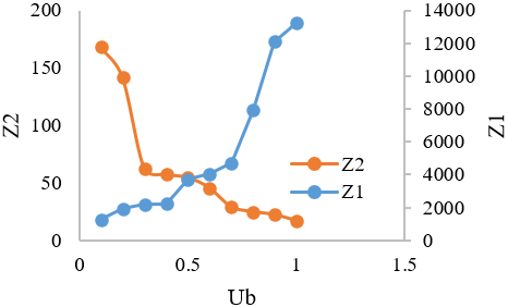
To carry out a sensitivity analysis, the model is analyzed by the total weight method with weights w1=w2=0.5 and by changing the value of ubip. Figure 2 depicts the sensitivity analysis results.
Figure 2. Sensitivity analysis of ub
According to Figure 2, variable Bivp will have more freedom of action for each node based on the desired product demand if the value of ubip is changed. Therefore, routes and time to stay in nodes are determined such that the value of ubip is maximized. This leads to an increase in the maximum arrival time (i.e., Cmax). On the other hand, this freedom of action will reduce the final costs because of less use of mobile factories. Meanwhile, a decrease in the amount of ubip causes no change in the Cmax value, which is probably because the model uses its maximum power to reduce the maximum of the whole system due to a fixed amount of αvp parameter and lack of excessive stay in nodes, which results in upper bound of other nodes. Overall, given these results, it can be concluded that this model is efficient in decreasing customer waiting time and production costs. The precision of this model is also affirmed given the presented example and its outcomes. Thus, it can be stated that this new mathematical model for the integration of production and distribution in mobile centers is efficient and could be applied by respective companies.
Integration of scheduling of production and distribution stages at the operational level for mobile factories to reduce operating costs and reduce the waiting time for the customer to receive the desired product is one of the most important factors for the success of a company. Nevertheless, several models focusing on problems of integrated production and distribution scheduling only evaluate decision-making at strategic or tactical levels, and a few of them have paid attention to integrated decisions at operational levels. The present study aimed to evaluate the production and distribution scheduling of mobile factories at the operational level as an innovation. To this end, a novel mathematical model was proposed for an integrated production and distribution scheduling problem by considering some real-world features, which focused on a decrease in the customer waiting time in addition to the reduction of production costs. A small-scale problem was solved to test the model’s accuracy. According to the results, the model can be used by all organizations that produce and distribute perishable products, such as dairy and pharmaceutical products, chemical compounds, and masks during the COVID-19 pandemic.
[1] Behzad, A., Pirayesh, M.A. (2016). Design of a mobile factory supply chain network. In the Second International Conference on Industrial and Systems Engineering (ICISE, 2016), Mashhad, Iran.
[2] Adulyasak, Y., Cordeau, J.F., Jans, R. (2015). The production routing problem: A review of formulations and solution algorithms. Computers & Operations Research, 55: 141-152. https://doi.org/10.1016/j.cor.2014.01.011
[3] Fu, L.L., Aloulou, M.A., Triki, C. (2017). Integrated production scheduling and vehicle routing problem with job splitting and delivery time windows. International Journal of Production Research, 55(20): 5942-5957. https://doi.org/10.1080/00207543.2017.1308572
[4] Lei, C., Lin, W. H., Miao, L. (2016). A two-stage robust optimization approach for the mobile facility fleet sizing and routing problem under uncertainty. Computers & Operations Research, 67: 75-89. https://doi.org/10.1016/j.cor.2015.09.007
[5] Halper, R., Raghavan, S., Sahin, M. (2015). Local search heuristics for the mobile facility location problem. Computers & Operations Research, 62: 210-223. https://doi.org/10.1016/j.cor.2014.09.004
[6] Raghavan, S., Sahin, M., Salman, F.S. (2019). The capacitated mobile facility location problem. European Journal of Operational Research, 277(2): 507-520. https://doi.org/10.1016/j.ejor.2019.02.055
[7] Halper, R., Raghavan, S. (2011). The mobile facility routing problem. Transportation Science, 45(3): 413-434. https://doi.org/10.1287/trsc.1100.0335
[8] Mohammadi, S., Al-e-Hashem, S.M., Rekik, Y. (2020). An integrated production scheduling and delivery route planning with multi-purpose machines: A case study from a furniture manufacturing company. International Journal of Production Economics, 219: 347-359. https://doi.org/10.1016/j.ijpe.2019.05.017
[9] Lei, C., Lin, W.H., Miao, L. (2014). A multicut L-shaped based algorithm to solve a stochastic programming model for the mobile facility routing and scheduling problem. European Journal of Operational Research, 238(3): 699-710. https://doi.org/10.1016/j.ejor.2014.04.024
[10] Friggstad, Z., Salavatipour, M.R. (2011). Minimizing movement in mobile facility location problems. ACM Transactions on Algorithms (TALG), 7(3): 28. https://doi.org/10.1145/1978782.1978783
[11] Singgih, I.K. (2020). Mobile laboratory routing problem for Covid-19 testing considering limited capacities of hospitals. In 2020 3rd International Conference on Mechanical, Electronics, Computer, and Industrial Technology (MECnIT), Medan, Indonesia, pp. 80-83. https://doi.org/10.1109/MECnIT48290.2020.9166664
[12] Low, C., Chang, C. M., Li, R.K., Huang, C.L. (2014). Coordination of production scheduling and delivery problems with heterogeneous fleet. International Journal of Production Economics, 153: 139-148. https://doi.org/10.1016/j.ijpe.2014.02.014
[13] Liu, P., Lu, X. (2016). Integrated production and job delivery scheduling with an availability constraint. International Journal of Production Economics, 176: 1-6. https://doi.org/10.1016/j.ijpe.2016.03.006
[14] Soukhal, A., Oulamara, A., Martineau, P. (2005). Complexity of flow shop scheduling problems with transportation constraints. European Journal of Operational Research, 161(1): 32-41. https://doi.org/10.1016/j.ejor.2003.03.002
[15] Hassanzadeh, A., Rasti-Barzoki, M., Khosroshahi, H. (2016). Two new meta-heuristics for a bi-objective supply chain scheduling problem in flow-shop environment. Applied Soft Computing, 49: 335-351. https://doi.org/10.1016/j.asoc.2016.08.019
[16] Güden, H., Süral, H. (2019). The dynamic p-median problem with mobile facilities. Computers & Industrial Engineering, 135: 615-627. https://doi.org/10.1016/j.cie.2019.06.024
[17] Akgün, İ., Erdal, H. (2019). Solving an ammunition distribution network design problem using multi-objective mathematical modeling, combined AHP-TOPSIS, and GIS. Computers & Industrial Engineering, 129: 512-528. https://doi.org/10.1016/j.cie.2019.02.004
[18] Ahmadi, S., Amin, S.H. (2019). An integrated chance-constrained stochastic model for a mobile phone closed-loop supply chain network with supplier selection. Journal of Cleaner Production, 226: 988-1003. https://doi.org/10.1016/j.jclepro.2019.04.132
[19] Ebrahimi, S.B., Bagheri, E. (2022). Optimizing profit and reliability using a bi-objective mathematical model for oil and gas supply chain under disruption risks. Computers & Industrial Engineering, 163: 107849. https://doi.org/10.1016/j.cie.2021.107849
[20] Rimélé, A., Gamache, M., Gendreau, M., Grangier, P., Rousseau, L.M. (2022). Robotic mobile fulfillment systems: A mathematical modelling framework for e-commerce applications. International Journal of Production Research, 60(11): 3589-3605. https://doi.org/10.1080/00207543.2021.1926570