Applications of Numerical Integrations on the Trapezoidal and Simpson's Methods to Analytical and MATLAB Solutions

In this study, we will present selected methods of numerical solution which focus on the performance of good approximation methods to benefit from approximation solutions aimed at trapezoidal method, Simpson's methods, accurate analytical solution and MATLAB. In this regard it is suffices to compare performance in terms of numerical accuracy and calculation error. Let us offer solutions to solve various problems.

2.1 Trapezoidal base

Task n=1 in the general formula:

$\int_{x_0}^{x_n} y d x=n h\left[y_0+\frac{n}{2} \Delta y_0+\frac{n(2 n-3)}{12} \Delta^2 y_0+\frac{n(n-2)^2}{24} \Delta^3 y_0+\cdots\right]$

All the top first differences will be zero, and we'll get them:

$\int_{x_0}^{x_1} y d x=h\left[y_0+\frac{1}{2} \Delta y_0\right]=h\left[y_0+\frac{1}{2}\left(y_1+y_0\right)\right]=\frac{h}{2}\left(y_0+y_1\right)$

For the next interval [x₁, x₂] we conclude in a similar way:

$\int_{x_1}^{x_2} y d x=\frac{h}{2}\left(y_1+y_2\right)$

And so on. For our last interval [x_n-1, x_n] we have:

$\int_{x_{n-1}}^{x_n} y d x=\frac{h}{2}\left(y_{n-1}+y_n\right)$

Combining the express, we develop law:

$\int_{x_0}^{x_n} y d x=\frac{h}{2}\left(y_0+2\left(y_1+y_2+\cdots+y_{n-1}\right)+y_n\right)$

which is known as a trapezoid law.

2.2 Simpson 1⁄3 rule

This rule is obtained if we put n=2, as in the formula

$\int_{x_0}^{x_n} y d x=n h\left[y_0+\frac{n}{2} \Delta y_0+\frac{n(2 n-3)}{12} \Delta^2 y_0+\frac{n(n-2)^2}{24} \Delta^3 y_0+\cdots\right]$

Replace the curve with n⁄2 quadratic or equivalent polynomial arcs.

We have what:

$\int_{x_0}^{x_2} y d x=2 h\left[y_0+\frac{1}{2} \Delta y_0+\frac{1}{6} \Delta^2 y_0\right]=\frac{h}{3}\left[y_0+4 y_1+y_2\right]$

Similarity

$\int_{x_2}^{x_4} y d x=\frac{h}{3}\left[y_2+4 y_3+y_4\right]$

Ultimately

$\int_{x_{n-2}}^{x_n} y d x=\frac{h}{3}\left[y_{n-2}+4 y_{n-1}+y_n\right]$

Summarize, we get it:

$\begin{aligned} \int_{x_0}^{x_n} y d x= & \frac{h}{3}\left(y_0+4\left(y_1+y_3+y_5+\cdots+y_{n-1}\right)\right. \\ & \left.+2\left(y_2+y_4+y_6+\cdots+y_{n-2}\right)+y_n\right)\end{aligned}$

which is commonly known as Simpson 1⁄3.

2.3 Simpson 3⁄8 rule

Setting n=3 in equation:

$\begin{aligned} \int_{x_0}^{x_n} y d x= & n h\left[y_0+\frac{n}{2} \Delta y_0+\frac{n(2 n-3)}{12} \Delta^2 y_0\right.  \left.+\frac{n(n-2)^2}{24} \Delta^3 y_0+\cdots\right]\end{aligned}$

Notice that all variations above the third become equal to zero, and we get them:

$\begin{aligned} \int_{x_0}^{x_3} y d x= & 3 h\left[y_0+\frac{3}{2} \Delta y_0+\frac{3}{4} \Delta^2 y_0+\frac{1}{8} \Delta^3 y_0\right] \\ & =3 h\left[y_0+\frac{3}{2}\left(y_1-y_0\right)\right. \\ & +\frac{3}{4}\left(y_2-2 y_1+y_0\right)+\frac{1}{8}\left(y_3-3 y_2+3 y_1\right. \\ & \left.\left.-y_0\right)\right]=3 h / 8\left(y_0+3 y_1+3 y_2+y_3\right)\end{aligned}$

In the same way:

$\int_{x_0}^{x_3} y d x=\frac{3 h}{8}\left(y_3+3 y_4+3 y_5+y_6\right)$

And so on. Summing up all this, we get it:

$\begin{array}{rl}\int_{x_0}^{x_n} y & d x=\frac{3 h}{8}\left[\left(y_0+3 y_1+3 y_2+y_3\right)\right. \\ & +\left(y_3+3 y_4+3 y_5+y_6\right)+\cdots \\ & \left.+\left(y_{n-3}+3 y_{n-2}+3 y_{n-1}+y_n\right)\right] \\ & =3 h / 8\left(y_0+3 y_1+3 y_2+2 y_3+3 y_4\right. \\ & +3 y_5+2 y_6+\cdots+2 y_{n-3}+3 y_{n-2} \\ & \left.+3 y_{n-1}+y_n\right)\end{array}$

This rule is called Simpson 3⁄8.

2.4 Exacting solutions

This section demonstrates the ability to solve overlapping generations of different algorithms using an accurate solution. Rather than converge in developing a multifaceted and detailed model for many practical reasons for real systems and provide a comprehensive analysis, we intend to describe the procedure to implement the solution of these algorithms and present its computational behavior. Not all functions have an analytical solution, with the help of this motivation we resort to approximate solutions.

2.5 MATLAB method

The MATLAB function attempts to approximate the integration of numerical function pleasure from the use of high-precision global adaptive quadrature and default error tolerance.

Example 1. Evaluate $\int_0^1 \frac{1}{1+x} d x$ by trapezoidal, Simpson 1⁄3 Rule and Simpson 3⁄8 Rule, also exciting and MATLAB solutions with h=0.25, and 0.125, respectively its shown in the results of Table 1 and graph 1.

When h=0.25, $y=f(x)=\frac{1}{1+x}$, x₀=0, y₀=1, x₁=0.25, y₁=0.8, x₂=0.50, y₂=0.6667, x₃=0.7, y3=0.5714, x₄=1, y₄=0.5.

By using trapezoidal rule

$\begin{aligned} \int_0^1 \frac{1}{1+X} & =\frac{h}{2}\left[y_0+y_4+2\left(y_1+y_2+y_3\right)\right] =\frac{0.25}{2}[1+0.5+2(0.8+0.6667+0.5714)]=0.6970\end{aligned}$

Using Simpson rule as 1⁄3

$\begin{aligned}

\int_0^1 \frac{1}{1+x}= & \frac{h}{3}\left[y_0+y_4+2\left(y_2\right)+4\left(y_1+y_3\right)\right]=\frac{0.25}{3}[1+0.52(0.6667)+4(0.8+0.5714)]=0.6932

\end{aligned}$

Using Simpson rule as 3⁄8

$\begin{aligned} \int_0^1 \frac{1}{1+x}= & \frac{3 h}{8}\left[y_0+y_4+2\left(y_3\right)+3\left(y_1+y_2\right)\right] =\frac{3(0.25)}{8}[1+0.5+2(0.5714)+3(0.8+0.6667)]=0.6602\end{aligned}$

Now h=0.125, $y=f(x)=\frac{1}{1+x}$, x₀=0, y₀=1, x₁=0.125, y₁=0.8889, x₂=0.250, y₂=0.8, x₃=0.375, y₃=0.7273, x₄=0.5, y4=0.6667, y₅=0.6154, x₅=0.625, x₆=0.750, y₆=0.5714, x₇=0.875, y₇=0.5333, x₈=1, y₈=0.5.

Trapezoidal results with Example 1

$\begin{aligned} & \int_0^1 \frac{1}{1+x}=\frac{h}{2}\left[y_0+y_8\right. + \left.2\left(y_1+y_2+y_3+y_4+y_5+y_6+y_7\right)\right] = \frac{0.125}{2}[1+0.5+2(0.8889+0.8 + 0.7273+0.667+0.6154+0.5714] = 0.6941\end{aligned}$

Simpson Rule 1⁄3 results

$\begin{aligned} & \int_0^1 \frac{1}{1+\mathrm{x}}=\frac{\mathrm{h}}{3}\left[\mathrm{y}_0+\mathrm{y}_8\right. + 2\left(\mathrm{y}_2+\mathrm{y}_4+\mathrm{y}_6\right)+4\left(\mathrm{y}_1+\mathrm{y}_3+\mathrm{y}_5+\mathrm{y}_7\right) = \frac{0.125}{3}[1+0.5+2(0.8+0.6667+0.5714) + 4(0.8889+0.7273+0.6154+0.5333]  =  0.6932\end{aligned}$

Simpson Rule 3⁄8 solutions

$\int_0^1 \frac{1}{1+x}=\frac{3 h}{8}\left[y_0+y_8\right.+2\left(y_3+y_6\right)+3\left(y_1+y_2+y_4+y_5\right.\left.\left.+y_7\right)\right]=\frac{3(0.125)}{8}[1+0.5+2(0.7273+0.5714)]+3(0.8889+0.8+0.6667+0.6154+0.5333)]=0.6848$

By Exacting solution for first example

$\int_0^1 \frac{1}{1+x} d x$

Let u=1+x, du=dx

$\int_0^1 \frac{1}{u} d u=\ln (u)_0^1=\ln (1+x)_0^1=\ln (1+1)-\ln (1+0)=\ln 2-\ln 1=0.6931-0=0.6931$

By using script will receiving the results:

clc

Cleae

Close all

Fun = @(x) 1 . /(1+x);

q=integral (fun, 0,1);

q=0.6931

Table 1. Numerical results with Simpson 1/3, Simpson3/8 and exacting

Discussion of three numerical outcomes with demanding arrangement and MATLAB on partial errors we understood Simpson 1/3 its best estimate to correct and MATLAB so he is the, winner with fragmentary capacity in Figure 1.

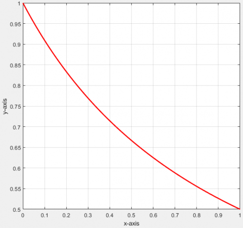
x=0: 0.001: 1

y=1 . /(1+x);

Plot (x, y, 'r', 'linewidth', 2);

Grid on

xlabel ('x-axis')

ylabel ('y-axis')

Example 2. Find the approximation value of $\int_0^\pi \sin x d x$ using three numerical methods trendy matlab solutions with $h=\frac{\pi}{6}$ and Simpson 1⁄3, Simpson 3⁄8 rules it will be represented in the Table 2 and Figure 2.

Solution of Trapezoidal rule

$y=f(x)=\int_0^\pi \sin x d x$

$x_0=0, y_0=0, x_1=\frac{\pi}{6}, y_1=0.5, x_2=\frac{\pi}{3}, y_2=0.8660$,$x_3=\frac{\pi}{2}, y_3=1, x_4=\frac{2 \pi}{3}, y_4=0.8660, x_5=\frac{5 \pi}{6}, y_5=0.5$,$x_6=\pi, y_6=0$.

By Trapezoidal Rule getting the results from example second

$\begin{aligned} \int_0^\pi \sin x d x= & \frac{h}{2}\left[y_0+y_6+2\left(y_1+y_2+y_3+y_4+y_5\right)\right. =\frac{\pi}{12}[0+0+2(0.5+0.8660+1+0.8660+0.5)]=1.9540\end{aligned}$ 

Simpson 1⁄3 rule results

$\begin{aligned}

& \int_0^\pi \sin x d x=\frac{h}{3}\left[y_0+y_6\right. \\

& \left.+2\left(y_2+y_4\right)+4\left(y_1+y_3+y_5\right)\right] \\

& =\frac{\pi}{18}[0+0+2(0.8660+0.86660) \\

& +4(0.5+1+0.5)]=2.0008

\end{aligned}$

Simpson 3⁄8 rule solution

$\int_0^\pi \sin x d x=\frac{3 h}{8}\left[y_0+y_6\right.\\

\left.+2\left(y_3\right)+3\left(y_1+y_2+y_4+y_5\right)\right]\\

=\frac{\pi}{16}[0+0+2(1)\\

+3(0.5+0.8660+0.8660+0.5)]=2.0019$

Exacting solution of example two

$\int_0^\pi \sin x d x=[-\cos x]_0^\pi=[-\cos \pi]-[-\cos 0]=2$

Using MATLAB script system as shown in Figure 1.

clc

Clear

Close all

Fun }=@(x) sin (x);

q=integral(fun, } 0,22 / 7);

q=2.0000

1.png

Figure 1. Trail of numerical solutions with the exact and MATLAB on distances of h=0.25

Table 2. The results of the second example are numerically solved with accurate and MATLAB solution

Exchange the estimates of numerical arrangements with a trapezoid on the sin function, include many disturbing errors but both are approaching strict and confused conformity, we note that Simpson's best digital technique from trapezoid to correct them in Figure 2.

x=0: 0.001: 22/7;

y=sin(x);

Plot(x,y,'r','linewidth', 2):

Grid on

2.png

Figure 2. Paths of label ('y-axis') and ('x-axis') responses the function thrut MATLAB

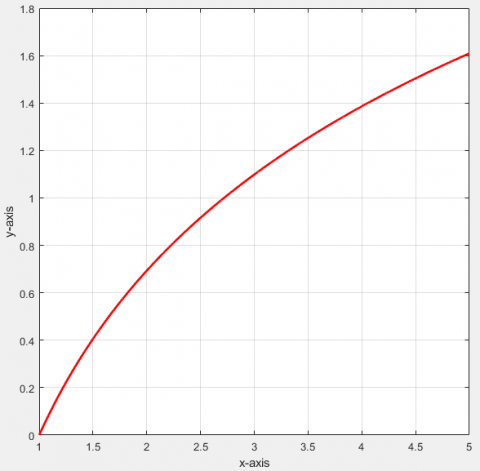
Example 3. Find the approximation value of $\int_1^5 \log x d x$ using Trapezoidal, Simpson 1⁄3, Simpson 3/8 rules in addition to the exact solu

With $h=0.5, y=f(x)=\int_1^5 \log x d x, x_0=1, y_0=0, x_1=1.5, y_1=0.4055, x_2=2, y_2=0.6931, x_3=2.5, y_3=0.9163, x_4=3, y_4=1.0986, x_5=3.5, y_5=1.2528, x_6=4, y_6=1.3863, x_7=4.5, y_7=1.5041, x_8=5, y_8=1.6094$.

Trapezoidal

$\int_1^5 \log x d x=\frac{h}{2}\left[y_0+y_8\right.$$\left.+2\left(y_1+y_2+y_3+y_4+y_5+y_6+y_7\right)\right]$$=\frac{0.5}{2}[0+1.6094$$+2(0.4055+06931+0.9163+1.0986$$+1.2528+1.3863+1.5041)]=4.0307$

Simpson 1⁄3

$\begin{array}{rl}\int_1^5 \log x & d x=\frac{h}{3}\left[y_0+y_8+2\left(y_2+y_4+y_6\right)\right. \\ & \left.+4\left(y_1+y_3+y_5+y_7\right)\right] \\ & =\frac{0.5}{3}[0+1.6094 \\ & +2(0.6931+1.0986+1.3863) \\ & +4(0.4055+0.9163+1.2528 \\ & +1.5041)]\end{array}$

Simpson 3⁄8

$\begin{array}{rl}\int_1^5 \log x & d x=\frac{h}{3}\left[y_0+y_8+2\left(y_2+y_4+y_6\right)\right. \\ & \left.+4\left(y_1+y_3+y_5+y_7\right)\right] \\ & =\frac{0.5}{3}[0+1.6094 \\ & +2(0.6931+1.0986+1.3863) \\ & +4(0.4055+0.9163+1.2528 \\ & +1.5041)]\end{array}$

Exacting solution

$\int_1^5 \log x d x=[x \log x-x]_1^5=(5 \log 5-5)-(1 \log 1-1)=4.0471$

MATLAB scrip results

clc

Clear

Closeall

Fun=@(x) \log (x)

q=integral(fun, 1,5)

q=4.0472

Table 3. The results from logarithmic function with numerical solutions, exact and MATLAB

Examine the logarithmic arrangement that we note from numerical outcomes, just Simpson 3/8 being adjusted away from numerical arrangements but other estimation techniques are great have about 0.160 decimal mistake, MATLAB in every case superior to anything and numerical errors has only 0.1 as apparently in Table 3.

Now, using MATLAB to explain the values through Figure 3.

x=0: 0.001: 5;

y=log(x);

Plot (x, y, 'r', 'linewidth', 2);

Grid on

xlabel ('x-axis')

ylabel ('y-axis')

3.png

Figure 3. Answer of the function with x-axes and y-axes by MATLAB

4.png

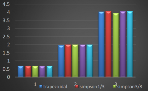
Figure 4. Comparing between Trapezoidal, Simpson 1/3, Simpson3/8, Exacting and MATLAB

Discussions of numerical methods it's come near mtalab solutions in exact order, we see that each of the formulas is settled through the different methods as shown in the models. The different outlines start from dark blue trapezoid to the light blue MATLAB, arrangement in three stages with five solutions. In the first step when h=0.25 the main model on all methods have a small error ratio less than one, in the second step of second formula with Simpson at h=0.52 We estimate the best numerical arrangements near specified order, in stage 3 of the model third h=0.5 trapezoid and Simpson 1/3 move towards a small number of errors but less than accurate in solutions as Simpson 3/8, column shows the green color is less accurate number, MATLAB recorded the best digital union where it contains an error very simple with the ability of the algorithmic equation a single decimal error number.