Muhammad Ridwan Andi Purnomo* | Dzuraidah Abdul Wahab | Ade Rizqy Anugerah
© 2022 IIETA. This article is published by IIETA and is licensed under the CC BY 4.0 license (http://creativecommons.org/licenses/by/4.0/).
OPEN ACCESS
This research aims to model and optimise the most applicable supply chain system, which is a single-vendor single-buyer system with fuzzy buyer demand. An optimisation model of the supply chain system under consideration is built by formulating the objective function, which is minimising the joint total cost between a buyer and a vendor. The model is developed on the basis of a simulation system, and optimisation is carried out by utilising a Genetic Algorithm that has been embedded in the simulation system. This technique is called optimisation–simulation closed loop. The vendor actual condition, which deals with uncertain demands from the main buyer and other small buyers, is considered. To analyse timely supply chain events, a simulation system is developed. A new optimisation model for the single-vendor single-buyer supply chain system with fuzzy demand is developed on the basis of the simulation system. The use of optimisation–simulation closed loop is also a new finding. In this study, the optimisation model of the supply chain under consideration is developed by taking into account a specific condition in which the vendor receives demands from the main buyer and other small buyers. Naturally, buyer demand is uncertain and has been modelled using a fuzzy set. The use of optimisation–simulation closed loop enables the supply chain to make the optimum decision when at the steady state condition.
single-vendor single-buyer, supply chain optimisation, fuzzy demand, optimisation–simulation closed loop, joint total cost
To ensure the efficiency and effectiveness of supply chain systems, attempts have been made to compile key performance indicators focusing on areas such as optimum supply chain configuration, inventory control, production quantity and flexibility increase. All of these objectives lead to the ultimate goal of the supply chain, that is, ensuring products are always available when needed at the lowest possible cost.
Due to their simplicity, most supply chain systems are beginning to lead to the single-vendor single-buyer supply chain system. The simpler the configuration, the simpler the cost structure and the lower the distribution cost. Furthermore, it allows a buyer to have a long-term relationship with a supplier, and the supplier gains experience to become more flexible than before. As in other supply chain systems, coordination between supply chain and uncertainty are the factors to consider in supply chain optimization [1].
Fu and Chien [2] investigated accurate forecasting to support supply chain resilience. To forecast demand, they developed a data-driven analytic framework that integrates machine learning technologies and a temporal aggregation mechanism. Belle et al. [3] studied the role of information sharing in accurate forecasting to support supply chain agility. According to Abolghasemi et al. [4], promotion can cause forecasting volatility, and the demand by promotion should be separated from the normal demand to accurately forecast it. They used statistics combined with machine learning technique for the demand forecasting.
Fuzzy logic (FL) is another technique that is widely used to model customer demand uncertainty. In FL, ambiguity is represented by a fuzzy curve. FL does not use clear or crisp logic to represent data domain membership. Data membership in a domain is determined strictly in crisp logic, which is false (0) or true (1). Crisp logic is not always appropriate for representing a condition in some systems. In a demand system, for example, if a clear rule says that ‘IF the demand quantity is >= 80, THEN the demand status is HIGH,’ then the status of a demand value of 80 units is HIGH. The status of a demand value at 79 units, by contrast, must not be HIGH. It is an unfair status because the effort to fulfil 80 or 79 units of demand is the same, and both demands can be classified to the same class. FL employs a membership value ranging from 0 to 1, rather than 0 or 1. As a result, the status of a demand at 80 units is HIGH with a degree of correctness of 100%, and that at 79 units is also HIGH with a degree of correctness of less than 100%. This outcome is logical.
Fuzzy curves have been used by several researchers to model and predict dynamic demand in supply chain systems. Sadeghi et al. [5] used a trapezoidal fuzzy set to represent fuzzy demand in a vendor managed inventory (VMI) system to optimise inventory. They used the centroid defuzzification method to predict the demand value. Malik and Kim [6] used a different fuzzy set, a triangular fuzzy number, to model fuzzy demand in a supply chain.
Coordination between the vendor and buyer is one of the factors for successful supply chain management in the single-vendor, single-buyer supply chain system [7]. A traditional management approach in such a system typically employs a push backward or reactive approach, in which the buyer optimises its decision and the result is pushed backward to the vendor. The vendor reacts to optimise its decision by referring to the optimum buyer decision. Such partial optimisation prevents the supply chain system from reaching its global optimum. When conducting optimisation, procurement from the buyer and production quantity in the vendor must be considered together to achieve global optimum conditions [8]. The integrated procurement and production quantity is known as joint economic lot size in supply chain optimisation, and it must be optimised concurrently to minimise joint total cost (JTC) between the vendor and buyer.
JTC is typically calculated by adding the total costs of the vendor and buyer. Several studies have looked into the JTC of the single-vendor single-buyer supply chain under various conditions. Wee and Widyadana [9] developed JTC by considering discrete delivery orders, random machine availability time that causes production delays and stock outs as lost sales. The optimum solution was obtained by deriving JTC. Lee and Kim [10] looked into JTC that resulted in total profit. They investigated deteriorating items and defective products during the manufacturing process. Braglia et al. [11] discussed safety stock management within the VMI context with consignment agreement. In addition to JTC, they also considered service level, which is usually just the logical result of JTC minimisation, in the optimisation.
Uncertainty has now become a common factor in supply chains, and supply chain researchers are paying close attention to it. Castellano et al. [12] investigated a study that considered uncertainty in demand and supply when optimising JTC. They found that an intermediate warehouse exists between the vendor and buyer, and queuing theory was used to model the system. Another technique that is usually used to model uncertainty is statistical distribution, which has been implemented in single-vendor multi-buyer supply chain coordination [13].
Most studies on supply chain JTC optimisation use a classical derivation approach. When JTC cannot be optimised through JTC derivation, the optimisation is performed in an iterative step known as an algorithm. In addition to the algorithm, intelligent optimisation techniques are used. Sue-Ann et al. [14] used an evolutionary algorithm to optimise common parameter values in a two-tier supply chain system. Nia et al. [15] used a hybridised Genetic Algorithm (GA) with an imperialist competitive algorithm to optimise a green VMI system under shortage conditions. Tarhini et al. [16] discussed the use of GA to optimise a supply chain system with buyer-to-buyer transshipments. The use of intelligent optimisation techniques in supply chain optimisation has received major attention from researchers, as the complexity of supply chain systems continues to rise.
Our study focuses on the optimisation of the single-vendor single-buyer supply chain system. Batik, a popular product in Indonesia, is the product of the investigated system. To deliver the product from the vendor to the buyer, the supply chain system employs a third-party logistic (TPL) system. In the supply chain system under consideration, several small buyers and one main buyer exist, and the vendor has a contract with the main buyer to supply the product as needed. Uncertainty demand from customers is modelled using FL in the main buyer, and unfulfilled demand is considered lost sales. Buyer decision variables are the reorder point and order quantity, which are vendor demands. To obtain a realistic product flow from time to time and because optimisation must be performed simultaneously in the vendor and buyer, an optimisation–simulation closed loop is used as the optimisation tool.
Previous studies on the single-vendor single-buyer supply chain system are reviewed in this section to distinguish this study from others. The review focuses on the supply chain system characteristics and the optimisation methods used. Ben-Daya and Hariga [17] investigated JTC minimisation with deterministic demand and lead time varying linearly with lot size. Following JTC formulation, a heuristic algorithm is proposed to determine the optimum lot size for the vendor and buyer, including the reorder point for the buyer. Three scenarios are presented to demonstrate that the proposed heuristic algorithm outperforms local optimisation for the vendor and buyer.
Benkherouf and Omar [18] presented a method for minimising JTC by determining the best buyer replenishment and vendor production schedule. Time-varying demand was modelled linearly subject to time, and JTC was minimised by substituting several equations into the objective function. Jaggi and Arneja [19] created a model for unstable lead time and setup cost with different vendor and buyer objectives. The vendor goal was to reduce setup costs, whereas the buyer goal was to reduce lead time. To validate the developed model, stochastic demand during lead time was modelled using a statistical approach, and case studies with complete and partial demands during lead-time information were presented.
Taleizadeh et al. [20] investigated JTC minimisation with stochastic demand and fuzzy lead time. Stochastic demand was represented by a statistical distribution, whereas fuzzy lead time was represented by membership value-based fuzzy simulation. They performed optimisation by using a continuous review inventory model with order quantity and reorder point as decision variables. Rad et al. [21] discussed the topic of joint profit maximisation. They pointed out that buyer demand is sensitive to selling price; therefore, selling price is one of the decision variables considered, along with order quantity and number of shipments. The optimisation tool was a simple iterative procedure. Vijayashree and Uthayakumar [22] conducted research on ordering cost reduction based on lead time. They considered two types of ordering cost: linear and logarithmic. To reduce the JTC of the supply chain system, solution procedures or algorithms were also proposed.
Jauhari [23] studied about JTC minimisation by considering safety factor, delivery lot size, delivery frequency, production rate and process quality. Imperfect production system, which affects vendor production quantity, was also considered by incorporated quality improvement factor in the analysis. Stochastic demand was considered, but only mean demand value was used in the proposed model. Trial and error simulation were implemented for seeking the decision variable value. Sekar and Uthayakumar [24] explored the imperfect production process. They considered multiple production runs with production setup, number of deliveries and lot size as decision variables. A classical derivation was performed to optimise the proposed JTC.
In this study, a single-vendor single-buyer supply chain system, which uses a TPL system to deliver products, is considered. Given that such a system calculates shipping cost on the basis of shipment weight, the buyer ordering cost is subject to its order quantity. The buyer uncertainty demand is modelled using a trapezoidal fuzzy number. The vendor responds to the buyer demand in several production batches, and given that the vendor has a consignment with the buyer, stock out results in a penalty cost. An optimisation–simulation closed loop system is implemented to optimise the supply chain system under consideration. In this loop system, a GA is used as the optimisation algorithm. The significant differences between this study and similar works are shown in Table 1.
Table 1. Differences between the current study and similar works
|
Author(s) |
Stochastic Demand Model |
Intelligent Optimisation |
Simulation Feedback |
Multiple Production Lot |
Continuous Review Inventory |
Variable Ordering Cost |
|
[17] |
|
|
|
|
√ |
|
|
[18] |
√ |
|
|
|
|
|
|
[19] |
√ |
|
|
|
√ |
|
|
[20] |
√ |
|
|
|
√ |
|
|
[21] |
√ |
|
|
√ |
|
|
|
[22] |
√ |
|
|
|
√ |
|
|
[23] |
|
|
|
|
√ |
|
|
[24] |
√ |
|
|
√ |
|
|
|
[16] |
√ |
√ |
|
|
√ |
|
|
This study |
√ |
√ |
√ |
√ |
√ |
√ |
This section explains the notations that represent the parameters and decision variables of the investigated supply chain system. It also defines fuzzy modelling for buyer demand, JTC modelling and the mechanism of the proposed optimisation–simulation closed loop.
3.1 Notations
General notations:
b: index for buyer
v: index for vendor
t: time index
h: inventory holding cost per unit per year (IDR/year)
H: total holding cost per unit per year (IDR/year)
$\bar{I}$: average inventory (units)
L: total lost sales cost (IDR)
I: inventory level (units)
Buyer notations:
ir: inventory level when receiving an order (units)
Ir: inventory level after receiving an order (units)
O: total ordering cost (IDR/order)
lt: ordering lead time (days)
Q: order quantity (units)
CT: inventory cycle time (days)
r: reorder point (units)
w: weight of shipped product per unit (kg)
S: shipment cost per kilogram charged by TPL (IDR/kg)
D: annual demand (units)
d: demand (units)
Dl: demand during lead time (units)
$\widetilde{f d}$: fuzzy demand (units)
$d_1$: the lowest demand that has ever occurred (units)
$d_2$: lower limit of demand interval that frequently occurs (units)
$d_3$: upper limit of demand interval that frequently occurs (units)
$d_4$: the highest demand that has ever occurred (units)
$\mu$: fuzzy membership value of a demand
$\pi$: lost sales cost per unit (IDR/unit)
Vendor notations:
TS: total setup cost (IDR)
St: setup cost per production batch (IDR/setup)
m: number of production lots
PCT: production cycle
$\widetilde{f D}$: fuzzy demand from other buyers (units)
$\pi_1$: lost sales cost (IDR/unit)
$\pi_2$: penalty cost for unfulfilled order (IDR/unit)
LS: production batch size (units)
Ir: total production lot size (Ir = LS x m)
ip: inventory level after fulfilling an order from a buyer (units)
TC: total cost (IDR)
l: lost sales cost in a production cycle (IDR/unit)
y: penalty cost in a production cycle (IDR/unit)
LP: total lost sales and penalty cost (IDR)
GA notations:
p_size: GA population size
G: GA’s number of generations
pc: GA crossover probability
pm: GA mutation probability
sp: number of super chromosomes in a population
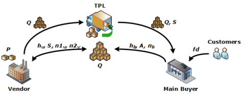
Figure 1 illustrates the supply chain system under consideration.
Based on Figure 1, after receiving the order quantity from the main buyer, the vendor uses it as a reference in determining optimum production quantity. Once the products are finished, they are delivered to the buyer via a TPL system. The TPL system determines the shipment cost on the basis of the shipment weight, and the shipment cost is considered the buyer ordering cost.
Figure 1. Diagram of supply chain system under consideration
In traditional supply chain management, one of the decision making is inventory optimisation [25, 26], therefore, the buyer optimises the reorder point and order quantity by considering demand during lead time, inventory holding cost, ordering cost and lost sales cost. The order quantity is the vendor demand, and the vendor optimises the number of production batches by considering inventory holding cost, setup cost, lost sales cost and penalty cost due to consignment. In this study, the reorder point, order quantity and number of production batches are optimised at a time whilst considering all of the supply chain system parameters.
3.2 Buyer fuzzy demand model
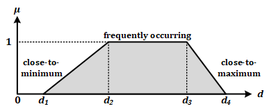
Naturally, customer demand received by the main buyer is uncertain, and it follows one of the following three patterns: frequently occurring, close-to-minimum and close-to-maximum. Such patterns are vague; therefore, the demand is modelled with trapezoidal fuzzy values to account for this vagueness. Figure 2 depicts the use of a trapezoidal fuzzy set to model the buyer demand. The trapezoidal fuzzy set is proposed because it represents a typical demand behaviour with frequent, minimum and maximum value. Company marketing managers can assist in determining d1, d2, d3 and d4 values on the basis of historical demand data. Since the managers already have demand management experiences, even though d1, d2, d3 and d4 values are subjectively determined, the managers’ common sense will reduce the variation of the d1, d2, d3 and d4 values.
Figure 2. Trapezoidal fuzzy set to represent the buyer fuzzy demand
The historical demand data is technically organised into intervals. In this study, frequently occurring intervals are defined as those containing more than sixty percent of the data whereas close-to-minimum and close-to-maximum intervals each cover twenty percent of the data. The demand value can be estimated using the defuzzification method. One of the defuzzification methods that is commonly used by researchers is centroid method, as formulated in Eq. (1) [27]. See the general notation section to find the definition of each variable.
$\widetilde{f d_b}=\frac{\int_{d_1}^{d_4} \mu_b \times d_b}{\int_{d_1}^{d_4} \mu_b}$ (1)
The centroid method is able to produce fair result since it estimates the result based on the centre point of the used fuzzy sets. The output of the fuzzy demand model, as a result of the defuzzification method, is used as a reference to simulate demand during lead time.
3.3 Main buyer total cost model
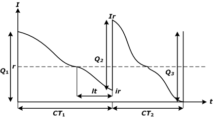
The main buyer total cost is calculated annually, assuming a year equals 360 days. Generally, the main buyer total cost consists of ordering cost, inventory holding cost and lost sales cost. Each of the total cost component will be explained based on the inventory graph that illustrated in Figure 3. The x-axis represents the inventory level (I) while the y-axis represents the time (t).
Figure 3. Inventory graph of the main buyer
Figure 3 shows that CT1 is shorter than CT2, implying that the demand rate in CT1 is lower than that in CT2. When I reaches r, the main buyer places a fixed-quantity order (Q) with the vendor. Stock outs are regarded as lost sales in the investigated supply chain system, and the lost sales formula is expressed by Eq. (4). As a result, in the inventory graph, the ir value when the main buyer receives the order will never be less than 0 units because stock in a period does not have to endure shortages in the past.
3.3.1 Total ordering cost
The total ordering cost is determined by the total shipment cost charged by the TPL. In this study, the shipment cost is per kg of shipment weight. The cost per shipment can be calculated by rounding up the total shipment weight and multiplying it by the cost per kg. The total shipment cost can then be calculated by multiplying the total cost per shipment by the shipment frequency, as presented in Eq. (2).
$O=\frac{\widetilde{f d}_b}{Q} \times(S \times\lceil Q \times w\rceil)$ (2)
3.3.2 Total inventory holding cost
Total inventory holding cost can be formulated as follows:
$H_b=\bar{I} \times h_b$$\bar{I}=i r+\frac{1}{2}(Q)$$\bar{I}=i r+\frac{1}{2}(E(I r)-E(i r))$$i r=\max (0 ; r-D l)$$\bar{I}=\left\{\begin{array}{c}\frac{Q}{2}, r \leq D l \\ \frac{Q}{2}+r-D l, r>D l\end{array}\right.$ (3)
3.3.3 Total lost sales cost
Given that lost sales can occur in any CT, the total lost sales cost is calculated by multiplying the lost sales cost per unit by the estimated lost sales quantity multiplied by the number of CTs. Eq. (4) depicts the formula.
$L_b=\pi \times \frac{\widetilde{f d}_b}{Q} \times \max (0 ; D l-r)$ (4)
3.3.4 Main buyer total cost
The main buyer total cost is the sum of total ordering cost, total inventory holding cost and total lost sales cost, as shown in Eq. (5).
$T C_b=O+H_b+L_b$$=\frac{\widetilde{f d_b}}{Q} \times(S \times[Q \times w\rceil)+\bar{I} \times h_b$$+\pi \times \frac{\widetilde{f d}_b}{Q} \times \max (0 ; D l-r)$ (5)
3.4 Vendor total cost model
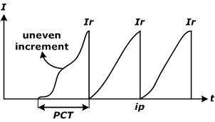
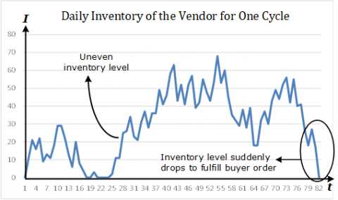
The vendor total cost is calculated annually. The initial inventory is assumed to be zero, and production can begin immediately. The vendor also deals with uncertain demands from other small buyers during the production process. This condition distinguishes the proposed model from the theoretical economic production quantity (EPQ), which assumes constant demand from the same buyer throughout production. As a result, inventory levels are uneven during the manufacturing process. Uncertain demands from small buyers are also modelled using fuzzy trapezoidal fuzzy numbers.
Figure 4. Vendor inventory graph
In this model, if the vendor production quantity is insufficient to fulfil the order from the main buyer, then it is considered a lost sale, and the vendor is penalised by the main buyer. When the main buyer demand is received and the production activity to meet that demand is completed, the product is shipped to the main buyer immediately, and the inventory level is drastically reduced. This condition also distinguishes the proposed model from the theoretical EPQ model, which assumes that inventory levels after production decrease linearly due to constant demand from the same buyers. In this study, production in a period does not have to endure the shortage in the past. As a result, the ip level in the vendor will never be lower than 0. The vendor inventory graph is illustrated in Figure 4.
3.4.1 Total setup cost
Total setup cost is the cost per production setup multiplied by the number of production batches and multiplied by the number of days per year, as shown in Eq. (6).
$T S=S t \times m \times 360$ (6)
3.4.2 Total inventory holding cost
The incorporation of the annual buyer demand in the vendor inventory holding cost model is one of the integration points between the vendor and buyer. The average inventory during PCT can be calculated using the inventory geometry displayed in Figure 4. The inventory holding cost is calculated by multiplying the inventory holding cost per unit per period by the average inventory during PCT, as presented in Eq. (7).
$P C T=\frac{Q}{D} \times 360$$H_v=h_v \times\left(i p+\frac{1}{P C T}\left(\sum_{t=1}^{P C T}((m \times L S)-\widetilde{f D})_t\right)\right)$$i p=\max \left(0 ; I r-d_v\right)$ (7)
3.4.3 Total lost sales and penalty cost
Sales are lost and penalties are incurred when the vendor production quantity is insufficient to meet the buyer demand. In this study, lost sales and penalty costs are per unit; thus, both costs can be added together and multiplied by the lost sales unit to calculate the total lost sales and penalty costs. Eq. (8) depicts a formula for calculating total lost sales and penalty costs.
$L_v=(l+y) \times \frac{d_v}{I r} \times \max \left(0 ; d_v-(m \times I r)\right)$. (8)
3.4.4 Vendor total cost
The vendor total cost is the sum of total setup cost, total inventory holding cost, total lost sales and penalty cost, as presented in Eq. (9).
$T C_v=T S+H_v+L_v=S t \times m \times 360+h_v \times$$\left(i p+\frac{1}{P C T}\left(\sum_{t=1}^{P C T}((m \times L S)-\widetilde{f D})_t\right)\right)+(l+y) \times$$\frac{d_v}{I r} \times \max \left(0 ; d_v-(m \times I r)\right)$. (9)
3.5 JTC
The supply chain system will not be able to achieve the global optimum solution if the total cost of the buyer and vendor is minimised separately. As a result, the total cost must be joined and used as the objective function in the optimisation process. Eq. (10) depicts the buyer and vendor JTC.
$J T C=T C_b+T C_v=O+H_b+L_b+T S+H_v+$$L_v==\frac{\widetilde{f d_b}}{Q} \times(S \times\lceil Q \times w\rceil)+\bar{I} \times h_b+\pi \times \frac{\widetilde{f d_b}}{Q} \times$$\max (0 ; D l-r)+S t \times m \times 360+h_v \times(i p+\left.\frac{1}{P C T}\left(\sum_{t=1}^{P C T}((m \times L S)-\widetilde{f D})_t\right)\right)+(l+y) \times \frac{d_v}{I r} \times\max \left(0 ; d_v-(m \times I r)\right)$. (10)
The optimisation objective function for JTC is minimisation with three decision variables, namely, Q, r and Ir (which is the function of LS and m). In JTC, r is affected by Q and Dl. Given that Q is a function of r, a circular reference exists between Q and r. Previous researchers typically solved this problem by using an initial Q value or developing a heuristic approach. No proof shows that the solution discovered is the best in either technique. In this study, JTC is optimised using an optimisation–simulation closed loop. A GA is proposed in the optimisation part, and the simulation is performed to obtain time series inventory analysis between the vendor and buyer.
The simulation initially generates $\widetilde{f d_b}, D L$ data by considering Q, m and r generated by GA. It then analyses the resulted $I_b$ and $S x_b$. Figure 5 shows the mechanism of the optimisation–simulation closed loop.
Figure 5. Optimisation–simulation closed loop mechanism to optimise the investigated supply chain system
The simulation system generates the parameter values (Fd and DL) to be fed into the GA. Then, GA optimises the decision variables (Q, r, m), which are fed back to the simulation system to calculate JTC on the basis of yearly simulation. The optimised variables change the parameter values for the next iteration. Such a process is iterated for a number of generations. This optimisation–simulation closed loop optimises the decision variables and validates the result simultaneously through a simulation process. This optimisation procedure causes the used GA to work with a fitness function whose values for dynamic variables are determined by simulation. It distinguishes the used GA from conventional GA that operate with a static fitness function.
This section discusses how the chromosome is formed in GA, including the compatible crossover and mutation operations on the chromosome.
4.1 Chromosome encoding and decoding
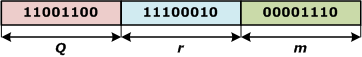
In GA, solutions to be found must be encoded in the form of chromosomes to enable GA to explore the solution domain by manipulating the chromosomes. The expected values for the decision variables in this study are integers, so binary encoding is used. For each decision variable, eight bits are provided to obtain precise values. Figure 6 depicts the binary-encoded chromosome, and Eq. (11) shows the formula for decoding the chromosome.
Figure 6. Binary-encoded chromosome to represent the solution
$Q=\operatorname{Min} V_Q+\operatorname{Int}\left(\frac{D V_Q}{255} \times\left(\operatorname{Max} V_Q-M i n V_Q\right)\right)$$r=M i n V_r+\operatorname{Int}\left(\frac{D V_r}{255} \times\left(\operatorname{Max} V_r-M i n V_r\right)\right)$$m=\operatorname{Min} V_m+\operatorname{Int}\left(\frac{D V_m}{255} \times\left(\operatorname{Max} V_m-M i n V_m\right)\right)$ (11)
4.2 Chromosome operation
Crossover is a binary operation that requires an even number of chromosomes. The number of chromosomes for crossover is controlled using crossover probability with random selection via random number generation. For a detailed description of the chromosome selection process for the crossover operation, see [28]. In our study, two crossover cut-points are used, as illustrated in Figure 7.
Figure 7. Two cut-point crossover mechanism
4.3 Mutation operation
One of the major issues discussed in GA is the local optimum trap caused by low chromosome diversity in a generation. When the chromosome diversity is low, the crossover operation is no longer effective in exploring the solution domain. The mutation operation, which is a unary operation, plays a major role in exploring the solution domain.
The main cause of low chromosome diversity is super chromosome dominance. When the gap between the super chromosome and the other chromosomes is large, the super chromosome is likely duplicated in the next generation, and the chromosome diversity decreases from generation to generation. To avoid this condition, the mutation rate in our study is determined dynamically on the basis of chromosome diversity. The formula for calculating the mutation rate is presented in Eq. (12).
$p_m=\frac{s p}{p_{-} \operatorname{size}}$ (12)
According to Eq. (12), when the population size is 30 and 3 super chromosomes are selected, the mutation rate is set to 0.1, which is relatively low. In another case, if 15 super chromosomes are chosen, then the mutation rate is set to 0.50, which is relatively high. The mutation process is carried out by generating a random number for every bit in every chromosome and if the generated random number is less than the pm, then the related but will be mutated. Given the high mutation rate, GA can have various chromosomes. Figure 8 shows how flip mutation is used in this study. For a detailed description of the chromosome selection process for the mutation operation, see Gen and Cheng (1998) [28].
Figure 8. Flip mutation mechanism
The case study took place at a batik retailer in Yogyakarta, Indonesia, as the buyer and the vendor are located in another city. The parameter values in the buyer were d1=105, d2=112, d3=115, d4=120, hb=25000, π=25000, lt=5 (days), Dl=0 to 7 units following a uniform distribution and S=50000. The parameter values in the vendor were St=100000, hv=10000, π1=10000, π2=15000 and LS= 5.
To ensure that the steady state condition was achieved, the simulation was run for 10 years (3,600 days) with the following GA parameter values: p_size=50; G=1000, pc=0.5; pm is dynamic as previously explained. The optimum supply chain condition after optimisation was Q=106 units, r=23 units and m = 3 with TCb=IDR 2.793.347,00, TCv=IDR 181.485.000,00 and JTC=IDR 184.278.347,00. Table 2 compares the results of push backward optimisation and the proposed joint optimisation.
Table 2. Comparison of push backward optimisation and the proposed joint optimisation
|
Opt. type |
Q |
r |
m |
TCb |
TCv |
JTC |
|
Push back |
315 |
18 |
4 |
4.456.111 |
145.882.500 |
150.338.611 |
|
Joint |
316 |
20 |
3 |
4.545.208 |
141.650.000 |
146.195.208 |
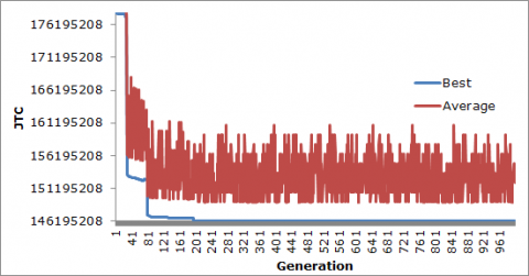
The quality of the GA searching process can be assessed on the basis of the GA ability to maintain chromosome diversity in each generation. It can be tracked using the GA searching process graph, as illustrated in Figure 9. According to the graph, the average fitness value is never the same as the best fitness value of the chromosome. That is, GA can maintain chromosome diversity in each generation. Moreover, the proposed GA is not trapped in a local optimum solution and can provide a global optimum solution.
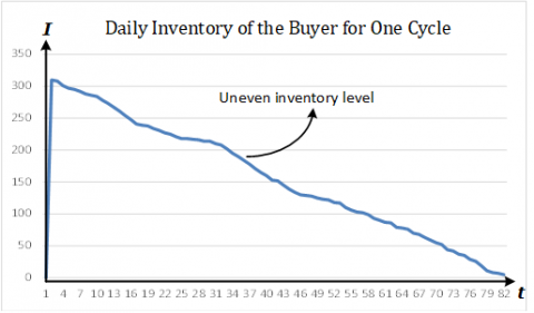
To validate the proposed model, it can be evaluated from the inventory movement patterns of the vendor and buyer and compared with the theoretical inventory pattern. Figures 10 and 11 present the inventory movement pattern of the vendor and buyer, respectively. As illustrated, the pattern is similar to the theoretical pattern.
Figure 9. GA searching process graph
Figure 10. Inventory movement pattern of the vendor for one cycle
Figure 11. Inventory movement pattern of the buyer for one cycle
Our study proposes the use of a continuous inventory review model for the buyer. According to the literature review, the majority of previous researchers used the same model, which monitors the inventory level on a regular basis. With this model, the supply chain system can achieve the lowest possible JTC.
This research has four major contributions: (1) the situation in which the vendor receives uncertain demands from other buyers during the production time, (2) the condition of the buyer inventory that drops immediately after shipping the products to the main buyer, (3) shipping cost that is a function of shipment weight and (4) the use of optimisation–simulation closed loop as the optimisation tool. Previous similar studies typically used estimated parameter values that did not accurately represent timely supply chain events.
A JTC model for the single-vendor single-buyer supply chain system has been developed by considering fuzzy demand from the main buyer and other small buyers, including the specific condition of the vendor inventory, which is drastically reduced after product delivery to the main buyer. Furthermore, the investigated supply chain system employs the TPL service for product delivery, with the shipment cost determined by shipment weight. All of these conditions distinguish the proposed JTC model from other similar models. Furthermore, the GA in the proposed optimisation–simulation closed loop performs well and can provide a global optimum solution.
According to the real supply chain system, which can have multiple product types, the model must be expanded by considering multiple product types and uncertainties in production lead time. The optimisation algorithm can also be changed to other intelligent optimisation algorithms, such as Bayesian optimisation, as it works on the basis of several data sampling and pattern result evaluation. Doing so can make the optimisation process faster than other evolution algorithms.
The authors would like to express their highest gratitude to the Department of Industrial Engineering, Universitas Islam Indonesia for funding the publication of this article.
[1] Gonçalves, J.N.C., Cortez, P., Carvalho, M.S., Frazao, N.M. (2021). A multivariate approach for multi-step demand forecasting in assembly industries: Empirical evidence from an automotive supply chain. Decision Support Systems, 142: 1-14. https://doi.org/10.1016/j.dss.2020.113452
[2] Fu, W., Chien, C.F. (2019). UNISON data-driven intermittent demand forecast framework to empower supply chain resilience and an empirical study in electronics distribution. Computers & Industrial Engineering, 135: 940-949. https://doi.org/10.1016/j.cie.2019.07.002
[3] Belle, J.V., Guns, T., Verbeke, W. (2021). Using shared sell-through data to forecast wholesaler demand in multi-echelon supply chains. European Journal of Operational Research, 288: 466-479. https://doi.org/10.1016/j.ejor.2020.05.059
[4] Abolghasemi, M., Beh, E., Tarr, G., Gerlach, R. (2020). Demand forecasting in supply chain: The impact of demand volatility in the presence of promotion. Computers & Industrial Engineering, 142: 1-12. https://doi.org/10.1016/j.cie.2020.106380
[5] Sadeghi, J., Mousavi, S.M., Niaki, S.T.A. (2016). Optimizing an inventory model with fuzzy demand, backordering, and discount using a hybrid imperialist competitive algorithm. Applied Mathematical Modelling, 40: 7318-7335. https://doi.org/10.1016/j.apm.2016.03.013
[6] Malik, A.I., Kim, B.S. (2020). A multi-constrained supply chain model with optimal production rate in relation to quality of products under stochastic fuzzy demand. Computers & Industrial Engineering, 149: 1-14. https://doi.org/10.1016/j.cie.2020.106814
[7] Liu, Y., Li, Q., Yang, Z. (2019). A new production and shipment policy for a coordinated single-vendor single-buyer system with deteriorating items. Computers & Industrial Engineering, 128: 492-501. https://doi.org/10.1016/j.cie.2018.12.059
[8] Ribas, I., Lusa, A., Corominas, A. (2021). Multi-step process for selecting strategic sourcing options when designing supply chains. Journal of Industrial Engineering and Management, 14(3): 477-495. https://doi.org/10.3926/jiem.3391
[9] Wee, H.M., Widyadana, G.A. (2013). Single-vendor single-buyer inventory model with discrete delivery order, random machine unavailability time and lost sales. International Journal of Production Economics, 143: 574-579. https://doi.org/10.1016/j.ijpe.2011.11.019
[10] Lee, S., Kim, D. (2014). An optimal policy for a single-vendor single-buyer integrated production–distribution model with both deteriorating and defective items. International Journal of Production Economics, 147: 161-170. https://doi.org/10.1016/j.ijpe.2013.09.011
[11] Braglia, M., Castellano, D., Frosolini, M. (2014). Safety stock management in single vendor–single buyer problem under VMI with consignment stock agreement. International Journal of Production Economics, 154: 16-31. https://doi.org/10.1016/j.ijpe.2014.04.007
[12] Castellano, D., Gebennini, E., Grassi, A., Murino, T., Rimini, B. (2018). Stochastic modeling of a single-vendor single-buyer supply chain with (s, S)-inventory policy. IFAC PapersOnLine, 51-11: 974-979. https://doi.org/10.1016/j.ifacol.2018.08.481
[13] Chan, C.K., Fang, F., Langevin, A. (2018). Single-vendor multi-buyer supply chain coordination with stochastic demand. International Journal of Production Economics, 206: 110–133. https://doi.org/10.1016/j.ijpe.2018.09.024
[14] Sue-Ann, G., Ponnambalam, S.G., Jawahar, N. (2012). Evolutionary algorithms for optimal operating parameters of vendor managed inventory systems in a two-echelon supply chain. Advances in Engineering Software, 52: 47-54. https://doi.org/10.1016/j.advengsoft.2012.06.003
[15] Nia, A.R., Far, M.H., Niaki, S.T.A. (2015). A hybrid genetic and imperialist competitive algorithm for green vendor managed inventory of multi-item multi-constraint EOQ model under shortage. Applied Soft Computing, 30: 353-364. https://doi.org/10.1016/j.asoc.2015.02.004
[16] Tarhini, H., Karam, M., Jaber, M.Y. (2020). An integrated single-vendor multi-buyer production inventory model with transshipments between buyers. International Journal of Production Economics, 225: 1-16. https://doi.org/10.1016/j.ijpe.2019.107568
[17] Ben-Daya, M., Hariga, M. (2004). Integrated single vendor single buyer model International Journal of Production Economics, 92: 75-80. https://doi.org/10.1016/j.ijpe.2003.09.012
[18] Benkherouf, L., Omar, M. (2010). Optimal integrated policies for a single-vendor single-buyer time-varying demand model. Computers and Mathematics with Applications, 60: 2066-2077. https://doi.org/10.1016/j.camwa.2010.07.047
[19] Jaggi, C.K., Arneja, N. (2011). Stochastic integrated vendor–buyer model with unstable lead time and setup cost. International Journal of Industrial Engineering Computations, 2: 123-140. https://doi.org/10.5267/j.ijiec.2010.06.001
[20] Taleizadeh, A.A., Niaki, S.T.A., Wee, H.M. (2013). Joint single vendor–single buyer supply chain problem with stochastic demand and fuzzy lead-time. Knowledge-Based Systems, 48: 1-9. https://doi.org/10.1016/j.knosys.2013.03.011
[21] Rad, M. A., Khoshalhan, F., Setak, M. (2014). Supply chain single vendor – single buyer inventory model with price - dependent demand. Journal of Industrial Engineering and Management, 7(4): 733-748. https://doi.org/10.3926/jiem.577
[22] Vijayashree, M., Uthayakumar, R. (2017). A single-vendor and a single-buyer integrated inventory model with ordering cost reduction dependent on lead time. Journal of Industrial Engineering International, 13(3): 393-416. https://doi.org/10.1007/s40092-017-0193-y
[23] Jauhari, W.A. (2017). A single-vendor single-buyer integrated production-inventory model with quality improvement and controllable production rate. Jurnal Teknologi, 80(1): 43-52. https://doi.org/10.11113/jt.v80.10494
[24] Sekar, T., Uthayakumar, R. (2018). A production inventory model for single vendor single buyer integrated demand with multiple production setups and rework. Uncertain Supply Chain Management, 6: 75-90. https://doi.org/10.5267/j.uscm.2017.6.001
[25] Mishra, N.K., Ranu. (2022). A supply chain inventory model for deteriorating products with carbon emission-dependent demand, advanced payment, carbon tax and cap policy. Mathematical Modelling of Engineering Problems, 9(3): 615-627. https://doi.org/10.18280/mmep.090308
[26] Setiawan, R., Salmah, Endrayanto, I., Indarsih. (2022). Analysis of a single manufacturer multi-retailer inventory competition using supermodular multi-objective games. Mathematical Modelling of Engineering Problems, 9(3): 559-567. https://doi.org/10.18280/mmep.090301
[27] Cox, E. (1999). The Fuzzy Systems Handbook A Practitioner’s Guide to Building, Using, and Maintaining Fuzzy Systems. Academic Press Inc, USA.
[28] Gen, M., Cheng, R. (1998). Genetic Algorithms and Engineering Optimisation. John Wiley and Sons, New York.