Funmilayo H. Oyelami* | Ebenezer O. Ige | Bidemi O. Falodun | Olaide Y. Saka-Balogun | Oluwaseyi A. Adeyemo
© 2022 IIETA. This article is published by IIETA and is licensed under the CC BY 4.0 license (http://creativecommons.org/licenses/by/4.0/).
OPEN ACCESS
In order to increase the drug potency and cancer treatment effectiveness, hyperthermia therapy is an adjuvant procedure in which perfused bodily tissues are heated to extreme temperatures. While certain types of hyperthermia treatments rely on thermal radiations from single-sourced electro-radiation measures, conjugating dual radiation field sources is being discussed in an effort to enhance the delivery of therapy. The thermal efficiency of a combined infrared hyperemia with nanoparticle recirculation near an applied magnetic field on subcutaneous strata of a model lesion as an ablation technique is investigated computationally in this research. To tackle the equation of linked momentum and thermal equilibrium in the blood-perfused tissue domain of a spongy fibrous tissue, an intricate Spectral relaxation method (SRM) was developed. The well-known Roseland diffusion approximation was used to define thermal diffusion regimes in the presence of external magnetic field imposition and to outline the effects of radiative flux inside the computational domain. Utilizing pore-scale porosity mechanics, the contribution of tissue sponginess was studied in a number of clinically relevant circumstances. Our findings demonstrated that magnetic field architecture could govern hemodynamic regimes at the blood-tissue interface across a significant depth of spongy lesion while permitting thermal transport across the depth of the model lesion. This parameter-indicator could be used to regulate how much hyperthermia therapy is administered to intravenously perfused tissue.
magneto-hemodynamic, infrared hyperthermia, spectra relaxation scheme, radiative flux
The development of thermal and non-thermal therapies for the diagnosis and treatment of tumor-related illnesses, however, is thought to have the potential to lessen the mortality load brought on by patients who are hampered by malignant infections. The potential of numerous techniques, including hyperthermic perfusion, conductive hyperthermia, electromagnetic and ultrasonic hyperthermia, and electrothermic operations, has led to the current optimism in the fight against cancer. This treatment is referred to as high temperature inducement of malignant region. For instance, according to experts in the field of oncology in Africa, Nigeria had the highest mortality rate in a study that was age-standardized [1].
Over the years, hyperthermia (HT) has played a significant role in the management of cancer-related illnesses. There have been documented innovations in the use of thermal biology to treat tumors at various anatomical places on the body. High temperature field exposure on areas of tumor growth is supplied to produce a curative effect on the tissue [2-4]. Application of thermal ablation is observed to precede and improve the potency of clinical interventions with far-reaching therapeutics effects such as chemotherapy, and radiotherapy [5, 6]. Time-based sustained thermal management of tumor growth around tissues with magnitude between 40℃ and 45℃ is a precursor for improved reperfusion within vasculature during radio and chemo based cancer treatment [7]. HT interventions are being achieved using selected avenues such as microwaves HT, radio HT, waves HT, ultrasound HT [2]. Whole body HT entails direct exposure on the entire body structure especially in cases of neoplasia which entails confiding the entire body heat loss while direct thermal inducement is made on skin and tissue to effect extracorporeal HT into the body core [8, 9]. The advancement around nanotechnology, introduction of nanoparticle in thermal inducement for therapeutics features in recent literatures. The presence of metallic nanoparticles around biological tissue is intended to generate hysteric heating around target tissue in the region of tumor. Embolizing ferromagnetic HT in external imposed magnetic field effect could be directed to minimize damage of healthy cells during cancer treatment [10].
Early reports have shown that externally imposed electromagnetic radiation frequency within the microwave range have the potential to induce localized heat effect on tumor growth either in the cutaneous and subcutaneous region of living organisms. Ali and Faramarz [11] described microwave HT device that could penetrate into subcutaneous tissue at elevate temperature. The study achieved microwave HT therapy on the abdominal wall of an anesthetized rat through multi-beam arrangements for explicit and precision heating around the region of malignancies. Nguyen et al. [12] reported a non-invasive HT strategy for mammalian cancer using microwave HT in a three-dimensional antenna-beam approach to describe electromagnetic wave penetration in breast cancer model. Nguyen et al. [13] experimentally showed that 65-W microwave HT penetration for breast cancer treatment by focusing 3D-antenna in the vicinity of tumor embedded in glands at elevated temperature 42℃ while keeping healthy tissue safe at 36℃ without any hot spots. During hyperthermia-type treatment in cancer issues, perfusion of blood across the vasculature of the diseased region is regarded because of its impact for circulation and removal of thermal energy in the vicinity of neighboring tissue. Numerical procedures have the capacity to predict and provide guidance to clinicians during administration of hyperthermia therapy in cancer patients.
In this investigation, a Chebyshev and pseudo-Spectral relaxation technique is used to investigate the effects of magnetic field-mediated radiative flux on infrared-type hyperthermia on a model of spongy tissue under perfusion. Our work reveals how biogenic fluid is transported through the perfused lesion's microvasculature. We present the first instance of a magnetic field being used to boost infrared-mediated hyperthermia on a field-based basis. While considering the perfusion in a near-native vascular spongy tissue with a predicted degree of porosity, researchers looked at the effects of regulated infrared radiation on a predetermined level of substrate lesion permeability.
Take into account the use of a magnetic field during hyperthermia therapy. In the study, the heat source is taken into account in order to act as an external device to raise the blood tissue's presumptive uniform temperature of 37℃. Convection, blood perfusion, thermal conduction, and metabolic heat creation are all combined in this heat transfer mechanism. The blood tissue motion was ignored in the earlier work [14]. As a result, the current work clarifies the momentum and thermal equilibrium between blood and tissue. This study makes the supposition that the local tissue's temperature and the blood's temperature throughout the tissue are comparable. Thus, the following are the one-dimensional momentum and energy equations:
$\frac{\partial u^*}{\partial t^*}=v \frac{\partial^2 u^*}{\partial y^{* 2}}-\frac{v}{K} u^*-\frac{\sigma B_O^2}{\rho} u^*$ (1)
$\rho_b C_{p b} \frac{\partial T^*}{\partial t^*}=K_b \frac{\partial^2 T^*}{\partial y^{* 2}} \omega_b \rho C_b\left(T_b-T\right)+Q_m\left(T^*-\right.$$\left.T_o\right)+\frac{\partial q_r}{\partial y^*}$ (2)
The boundary conditions are also:
$u^*\left(y^*, 0\right)=37^{\circ} \mathrm{C}$$u^*\left(0, t^*\right)=37^{\circ} \mathrm{C}$,
$u^*\left(a, t^*\right)=45^{\circ} \mathrm{C}$ (3)
$T^*\left(y^*, 0\right)=37^{\circ} \mathrm{C}$$T^*\left(0, t^*\right)=37^{\circ} \mathrm{C}$,
$T^*\left(a, t^*\right)=45^{\circ} \mathrm{C}$ (4)
The radiative heat flux is used to calculate the Rosseland diffusion approximation, which is defined as:
$q_r=\frac{-4 \sigma_s}{3 K_e} \frac{\partial T^{* 4}}{\partial y^*}$ (5)
where, Ke stands for mean absorption coefficient and σ is the Stefan-Boltzman constant. It is assumed that temperature changes inside the blood motion are sufficiently low when the Taylor series is used to expand T*4 and higher orders are neglected. As a result, T*4 which is the quartic temperature function may be represented as a linear function as shown below:
$T^{* 4} \cong 4 T_b^3 T^*-3 T_b^{* 4}$ (6)
Applying Eq. (6) to Eq. (2) to get:
$\frac{\partial q_r}{\partial y^*}=\frac{-16 \sigma_s T_b^{* 3}}{3 K_e} \frac{\partial^2 T^*}{\partial y^{* 2}}$ (7)
There are established non-dimensional functions given below:
$u=\frac{u^*}{v}, y=\frac{y^*}{v}, t=\frac{t^*}{v^2}, \theta=\frac{T^*-T_o}{T_b-T_o}$ (8)
Eqns. (1) and (2) in their dimensionless version become (1) and (2) by employing Eq. (8).
$\frac{\partial u}{\partial t}=\frac{\partial^2 u}{\partial y^2}-\frac{1}{K \rho} u-m u$ (9)
$\frac{\partial \theta}{\partial t}=\alpha\left(1+\frac{4}{3} R\right) \frac{\partial^2 \theta}{\partial y^2}+(r+\beta)-(r-\lambda) \theta$ (10)
where, $\zeta=a^2 \omega_b, \eta=\frac{Q m a^2}{\rho_b C_{p b}}, \alpha=\frac{K_b}{\rho_b C_{p b}}, \beta=\frac{\varepsilon a^2}{K \rho_b C_{p b}\left(T_b-T_0\right)}$.
The modified non-dimensional Eqns. (9) and (10) are answered using the SRM (10). By using the Gauss-Siedel relaxation strategy, this iterative method linearizes and decouples sets of nonlinear differential equations. After that, the Chebyshev pseudo-spectral method developed [15-17] is used to discretize the linear system of equations. The non-linear functions are presummated to exist at the previous step (r) whereas the linear functions are calculated at the most recent iteration step (r+1).
This approach (SRM) is special since it can resolve both ordinary and partial differential equations. Eqns. (11) and (12) are obtained by applying the SRM to the modified momentum and energy Eqns. (9) and (10).
$\frac{\partial u_{r+1}}{\partial t}=\frac{\partial^2 u_{r+1}}{\partial y^2}-\frac{1}{K_p} u_{r+1}-m u_{r+1}$ (11)
$\frac{\partial \theta_{r+1}}{\partial t}=\alpha\left(1+\frac{4}{3} R\right) \frac{\partial^2 \theta_{r+1}}{\partial y^2}+(\zeta+\beta)-(\zeta$$-\eta) \theta_{r+1}$ (12)
Depending on:
$u_{r+1}(y, 0)=37^{\circ} \mathrm{C}, u_{r+1}(0, t)=37^{\circ} \mathrm{C}$ (13)
$\theta_{r+1}(y, 0)=37^{\circ} \mathrm{C}, \theta_{r+1}(0, t)=37^{\circ} \mathrm{C}$ (14)
Setting: Setting: $\quad a_{0, r}=\frac{1}{K_p}, a_{1, r}=-m, b_{0, r}=\alpha\left(1+\frac{4}{3} R\right), b_{1, r}=$ $-(\zeta-\eta) ; b_{2, r}=(\beta+\zeta)$.
Substituting the above coefficient parameters into Eq. (11) and Eq. (12) to obtain:
$\frac{\partial u_{r+1}}{\partial t}=\frac{\partial^2 u_{r+1}}{\partial y^2}+a_{0, r} u_{r+1}+a_{1, r} u_{r+1}$ (15)
$\frac{\partial \theta_{r+1}}{\partial t}=b_{0, r} \frac{\partial^2 \theta_{r+1}}{\partial y^2}+b_{1, r} \theta_{r+1}+b_{2, r}$ (16)
Subject to Eq. (13) and Eq. (14).
We now define Gauss-Lobatto points according to [15-17] as:
$\Sigma_j=\cos \frac{\pi j}{N}, j=0,1,2, \ldots, N ; 1 \leq \xi \leq-1$ (17)
The physical neighborhood's realm is transformed from [0,1] to [-1,1], where N denotes the number of collocation points.
An early hunch on the boundary conditions is made as follows:
$u_0(y, t)=\theta_0(y, t)=37^{\circ} \mathrm{C}+e^{-\eta}-1$ (18)
As a result, the dimensionless Eqns. (9) and (10) were repeatedly solved for the unknown functions starting with the initial approximation defined in Eqns. (8) and (18). Whenever r=0, 1, 2, the iterative schemes (15) and (16) are solved iteratively for $u_{r+1}$(y, t) and $\theta_{r+1}$(y, t) respectively. The y-path equations will be discretized using the Chebyshev spectral collocation method, and the implicit difference method will be utilized to center the mid-point between tn+1 and tn.
The middle point is indicated by:
$t^{n+\frac{1}{2}}=\frac{t^{n+1}+t^n}{2}$ (19)
Thus, using the centering point about $t^{n+\frac{1}{2}}$ to the unidentified functions, say $u(y, t)$ and $\theta(y, t)$ with its associated derivative as noted [15] and defined in this study as:
$u\left(y_j, t^{n+\frac{1}{2}}\right)=u_j^{n+\frac{1}{2}}=\frac{u_j^{n+1}}{2},\left(\frac{\partial u}{\partial t}\right)^{n+\frac{1}{2}}=\frac{u_j^{n+1}-u_j^n}{\Delta t}$ (20)
$\theta\left(y_j, t^{n+\frac{1}{2}}\right)=\theta_j^{n+\frac{1}{2}}=\frac{\theta_j^{n+1}}{2},\left(\frac{\partial \theta}{\partial t}\right)^{n+\frac{1}{2}}=\frac{\theta_j^{n+1}-\theta_j^n}{\Delta t}$ (21)
We then use differential matrix D to apply the idea of the spectral collocation approach to estimate derivatives of unidentified variables given in Eqns. (22) and (23):
$\frac{d^r u}{d y^r}=\sum_{K=0}^N D_{i K}^r u\left(\varepsilon_K\right)=D^r u, i=0,1, \ldots, N$ (22)
$\frac{d^r \theta}{d y^r}=\sum_{K=0}^N D_{i K}^r \theta\left(\varepsilon_K\right)=D^r \theta, i=0,1, \ldots, N$ (23)
Applying Eqns. (22) and (23) on (15) and (16) before applying the finite difference scheme to obtain:
$\frac{d u_{r+1}}{d t}=u_{r+1} D^2+a_{0, r} u_{r+1}+a_{1, r} u_{r+1}$ (24)
$\frac{d \theta_{r+1}}{d t}=b_{0, r} D^2 \theta_{r+1}+b_{1, r} \theta_{r+1}+b_{2, r}+b_{3, r}$ (25)
Subject to:
$u_{r+1}\left(x_0, t\right)=37^{\circ} \mathrm{C}, u_{r+1}\left(x N_x, t\right)=37^{\circ} \mathrm{C}$ (26)
$\theta_{r+1}\left(x_0, t\right)=37^{\circ} \mathrm{C}, \theta_{r+1}\left(x N_x, t\right)=37^{\circ} \mathrm{C}$ (27)
Simplifying Eqns. (24) and (24) to obtain:
$\frac{d u_{r+1}}{d t}=\left(D^2+a_{0, r}+a_{1, r}\right) u_{r+1}$ (28)
$\frac{d \theta_{r+1}}{d t}=\left(b_{0, r} D^2+b_{1, r}\right) \theta_{r+1}+b_{2, r}$ (29)
We proceed to apply the finite difference scheme to obtain:
$\left(\frac{u_{r+1}^{n+1}-u_{r+1}^n}{\Delta t}\right)=\left(D^2+a_{o, r}+a_{1, r}\right)\left(\frac{u_{r+1}^{n+1}+u_{r+1}^n}{2}\right)$ (30)
$\left(\frac{\theta_{r+1}^{n+1}-\theta_{r+1}^n}{\Delta t}\right)=\left(b_{o, r} D^2+b_{1, r}\right)\left(\frac{\theta_{r+1}^{n+1}+\theta_{r+1}^n}{2}\right)+b_{2, r}$ (31)
Simplifying further to obtain:
$\left(\frac{1}{\Delta t}\right) u_{r+1}^{n+1}-\left(\frac{1}{\Delta t}\right) u_{r+1}^n=\left(\frac{D^2+a_{o, r}+a_{1, r}}{2}\right) u_{r+1}^{n+1}+$$\left(\frac{D^2+a_{o, r}+a_{1, r}}{2}\right) u_{r+1}^n$ (32)
$\left(\frac{1}{\Delta t}\right) \theta_{r+1}^{n+1}-\left(\frac{1}{\Delta t}\right) \theta_{r+1}^n=\left(\frac{b_{o, r} D^2+b_{1, r}}{2}\right) \theta_{r+1}^{n+1}+$$\left(\frac{b_{o, r} D^2+b_{1, r}}{2}\right) \theta_{r+1}^n+b_{2, r}$ (33)
Upon further simplification,
$\left(\frac{1}{\Delta t}\right) u_{r+1}^{n+1}-\left(\frac{D^2+a_{o, r}+a_{1, r}}{2}\right) u_{r+1}^{n+1}=\left(\frac{1}{\Delta t}\right) u_{r+1}^n+$$\left(\frac{D^2+a_{o, r}+a_{1, r}}{2}\right) u_{r+1}^n$ (34)
$\left(\frac{1}{\Delta t}\right) \theta_{r+1}^{n+1}-\left(\frac{b_{o, r} D^2+b_{1, r}}{2}\right) \theta_{r+1}^{n+1}=\left(\frac{1}{\Delta t}\right) \theta_{r+1}^n+$$\left(\frac{b_{o, r} D^2+b_{1, r}}{2}\right) \theta_{r+1}^n+b_{2, r}$ (35)
Simplifying further to obtain:
$\left[\left(\frac{1}{\Delta t}\right)-\left(\frac{D^2+a_{o, r}+a_{1, r}}{2}\right)\right] u_{r+1}^{n+1}=\left[\left(\frac{1}{\Delta t}\right)+\right.$$\left.\left(\frac{D^2+a_{o, r}+a_{1, r}}{2}\right)\right] u_{r+1}^n+K_1$ (36)
$\left[\left(\frac{1}{\Delta t}\right)-\left(\frac{b_{o, r} D^2+b_{1, r}}{2}\right)\right] \theta_{r+1}^{n+1}=\left[\left(\frac{1}{\Delta t}\right)+\right.$$\left.\left(\frac{b_{o, r} D^2+b_{1, r}}{2}\right)\right] \theta_{r+1}^n+K_2$ (38)
Hence, the iterative scheme becomes:
$P_1 u_{r+1}^{n+1}=Q_1 u_{r+1}^n+K_1$ (38)
$P_2 \theta_{r+1}^{n+1}=Q_2 \theta_{r+1}^n+K_2$ (39)
where,
$\begin{aligned} P_{1=} & {\left[\left(\frac{1}{\Delta t}\right)-\left(\frac{D^2+a_{o, r}+a_{1, r}}{2}\right)\right], Q_1 } \\ & =\left[\left(\frac{1}{\Delta t}\right)+\left(\frac{D^2+a_{o, r}+a_{1, r}}{2}\right)\right], K_1=0\end{aligned}$$\begin{aligned} P_2= & {\left[\left(\frac{1}{\Delta t}\right)-\left(\frac{b_{o, r} D^2+b_{1, r}}{2}\right)\right], Q_2 } \\ & =\left[\left(\frac{1}{\Delta t}\right)+\left(\frac{b_{o, r} D^2+b_{1, r}}{2}\right)\right], K_2=b_{2, r}\end{aligned}$
This study examined the effects of magnetic field strength on hyperthermia therapy using the SRM. The impacts of pertinent flow parameters were graphically depicted in order to study the model's physics. The Gauss Seidel methodology is used in this work's iterative numerical method to decouple the system's equations.
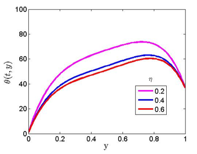
Figure 1 illustrates the impact of changing heat source characteristics on the temperature field. Membrane pumps cause the tissue to heat up, providing both the energy needed for chemical processes and for active transport. Convective heat diffusion throughout the blood and the tissue of the forearm is the crucial area where heat source in tissue plays a significant role. The blood works as a heat sink in a heated steady state of biased immersion in water at 38℃, transporting heat away from the limb; the quantity of heat gained from the area is minimal. When a result, the fluid temperature decreases as the heat source parameter is increased.
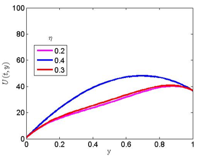
The effect of the heat source on velocity is seen in Figure 2. As the heat source parameter is increased, it is seen that the velocity plot expands.
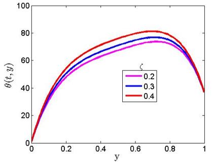
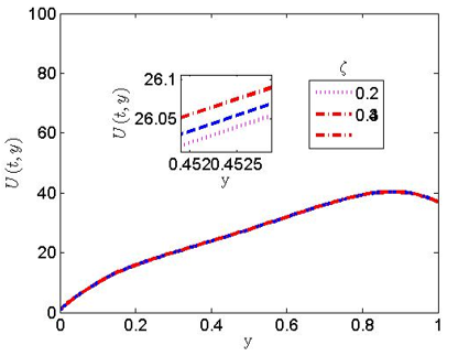
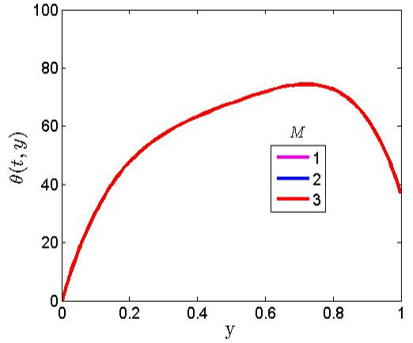
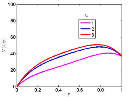
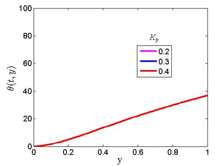
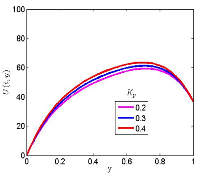
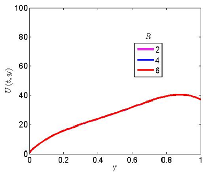
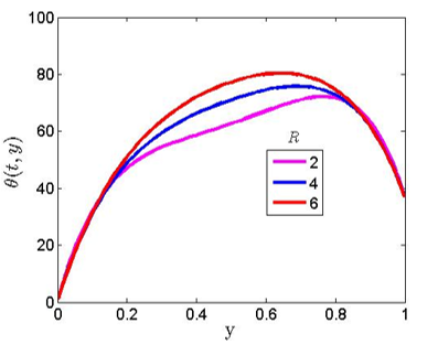
Figure 3 shows that the temperature distribution increases along with the blood perfusion parameter. It suggests that fluid velocity approaches its maximum as blood perfusion rises. This indicates that biological tissues rise and become linear at ζ=0.3, whereas they fall and become linear at ζ=0.1. Figure 4 demonstrates that raising the blood perfusion rate causes an increase in the fluid temperature of natural tissue for ζ=0.1, 0.2, and 0.3. By blocking the iliac artery, a pressure cuff is utilized to manage perfusion pressure. Direct measurement of blood flow temperature and velocity profile is the most common method for determining blood flow. It is important to understand that blood viscosity reduces at high temperatures, which causes the temperature plot to rise. The effect of a magnetic field on a temperature plot is seen in Figure 5. The increase in magnetic field does not seem to have any impact on the temperature profile. The impact of the magnetic field on the velocity plot is seen in Figure 6. It is demonstrated that as the magnetic parameter is raised, the velocity profile increases. This only shows that the Lorentz force, which causes the fluid velocity to decrease, is zero at the maximum magnetic value. This indicates that the velocity plot is strongly affected by the existence and application of the magnetic field parameter. The temperature field in Figure 7 is unaffected by the reaction of raising the permeability term. Figure 8 depicts how the porosity term responds to the velocity plot. As the porosity parameter rises, the velocity profile quickens. This is brought on by the increased movement of blood cells through the porous tissue. Figure 9 depicts the relationship between the radiation and the velocity plot. Raising the radiation term is shown to have no impact on the velocity plot. Figure 10 depicts how radiation affected the temperature plot. The temperature plot increases in response to increased radiation. The radiation parameter becomes more relevant at higher temperatures. Figure 11 illustrates how heat conductivity affects the velocity profile. It has been observed that the velocity profile increases along with the increase in heat conductivity.
Figure 1. The impact of the heat source on the temperature graph
Figure 2. The impact of heat source on velocity graph
Figure 3. The impact of blood perfusion on temperature graph
Figure 4. The impact of blood perfusion parameter on velocity graph
Figure 5. The impact of magnetic field on temperature graph
Figure 6. The impact of magnetic field on velocity graph
Figure 7. The impact of the porosity parameter on temperature graph
Figure 8. The impact of porosity parameter on velocity graph
Figure 9. The impact of radiation parameter on velocity graph
Figure 10. The impact of radiation parameter on temperature graph
Figure 11. The impact of thermal conductivity on velocity graph
Under the influence of the porosity term, a numerical investigation of the impact of radiative flux caused by magnetic and infrared hyperthermia has been conducted. While studying a heat source to use as an external device to intensify the temperature, we considered the blood tissue at a temperature of 37℃.
The following are the main conclusions reached following a thorough analysis of the issue. The temperature degrades as the heat source's value increases. When the temperature is high, the blood viscosity decreases, indicating an increase in the temperature plot. It was discovered that a greater magnetic value degenerated the velocity plot but had no bearing on the temperature profile while the blood cell's travel is accelerated by the permeable tissue.
It was discovered that increased thermal radiation increased the fluid temperature profile but had no impact on the velocity profile.
The authors are grateful to management of Afe Babalola University Ado-Ekiti Nigeria for providing facilities to conduct this research.
|
ζ |
Blood Perfusion |
|
ρb |
Ensity of Blood |
|
Cpd |
Specific Heat of Blood at Constant Temperature |
|
T |
Fluid Temperature |
|
Kb |
Thermal Conductivity of Blood |
|
ɷb |
Blood Volumetric Perfusion Rate |
|
υ |
Blood Perfusion Rate terms |
|
σ |
Stefan-Boltzmann Constant |
|
B0 |
Magnetic field constant |
|
t |
Time |
|
y |
Dimensionless Radial Coordinate |
|
K |
Thermal Conductivity |
|
ρ |
Fluid Density |
|
Cp |
Specific Heat at Constant Temperature |
|
Tb |
Temperature of Blood |
|
Qm |
Heat Source due to Metabolic Heat Generation in the Tissue |
|
To |
Reference Temperature (Tb>To) |
|
qr |
Radioactive Heat Flux |
|
µ |
Coefficient of Viscosity |
|
a |
Antenna Constant |
|
σs |
Macroscopic Scattering Cross-section |
|
ke |
Mean Absorpion Coefficient |
|
Cb |
Specific Heat of Blood |
|
R |
Radiation Parameters |
|
θ |
Dimensionless Temperature |
|
ε |
Porosity of the Tissue |
|
α |
Blood Thermal Conductivity Terms |
|
β |
Porosity Parameters |
|
r |
Spatial Coordinate |
|
η |
Heat Source Term |
|
Q |
Heat Source Term |
|
m |
Mass of Tissue |
|
Ec |
Eckert Number |
|
N |
Number of Collocation Points |
|
D |
Differential Matrix |
[1] Azubuike, S.O., Muirhead, C., Hayes, L., McNally, R. (2018). Rising global burden of breast cancer: The case of sub-Saharan Africa (with emphasis on Nigeria) and implications for regional development: A review. World Journal of Surgical Oncology, 16(1): 1-13. https://doi.org/10.1186/s12957-018-1345-2
[2] Behrouzkia, Z., Joveini, Z., Keshavarzi, B., Eyvazzadeh, N., Aghdam, R.Z. (2016). Hyperthermia: How can it be used? Oman Medical Journal, 31(2): 89-97. https://doi.org/10.5001/omj.2016.19
[3] Ankita, D., Vasu B., Anwar Bég, O., Gorla, R.S.R. (2021). Finite element computation of magneto-hemodynamic flow and heat transfer in a bifurcated artery with saccular aneurysm using the Carreau-Yasuda biorheological model. Microvascular Research, 138: 104221. https://doi.org/10.1016/j.mvr.2021.104221
[4] Ige, E.O., Oyelami, F.H., Adedipe, E.S., Tlili, I., Khan, M.I., Khan, S.U., Malik, M.Y., Xia, W.F. (2021). Analytical simulation of nanoparticle-embedded blood flow control with magnetic field influence through spectra homotopy analysis method. International Journal of Modern Physics B, 35(22): 2150226. https://doi.org/10.1142/S021797922150226X
[5] Al-Zu’bi, M., Mohan, A. (2020). Modelling of combination therapy using implantable anticancer drug delivery with thermal ablation in solid tumor. Scientific Reports, 10(1): 1-16. https://doi.org/10.1038/s41598-020-76123-0
[6] Shorif, A., Bablu, L., Manashjit, G., Haladhar, D. (2020). Magnetic nanoparticles mediated cancer hyperthermia. Smart Healthcare for Disease Diagnosis and Prevention, 153-173. https://doi.org/10.1016/B978-0-12-817913-0.00016-X
[7] Prasad, B., Kim, J.K., Kim, S. (2019). Role of simulations in the treatment planning of radiofrequency hyperthermia therapy in clinics. Journal of Oncology, 2019: 9685476. https://doi.org/10.1155/2019/9685476
[8] Ash, S.R. (1997). Extracorporeal whole body hyperthermia treatments for HIV infection and AIDS. ASAIO Journal, 43: M830-M838. https://doi.org/10.1097/00002480-199709000-00101
[9] Vertrees, R.A., Leeth, A., Girouard, M., Roach, J.D., Zwischenberger, J.B. (2002). Whole-body hyperthermia: A review of theory, design and application. Perfusion, 17(4): 279-290. https://doi.org/10.1191/0267659102pf588oa
[10] Moroz, P., Jones, S.K., Winter, J., Gray, B.N. (2001). Targeting liver tumors with hyperthermia: Ferromagnetic embolization in a rabbit liver tumor model. Journal of Surgical Oncology, 78(1): 22-29. https://doi.org/10.1002/jso.1118
[11] Ali, A.T., Faramarz, T. (2019). Numerical study of induction heating by micro / nano magnetic particles in hyperthermia Ali Asghar Journal of Computational and Applied Research in Mechanical Engineering, 9(2): 259-273.
https://doi.org/10.22061/JCARME.2019.3961.1465
[12] Nguyen, P.T., Abbosh, A., Crozier, S. (2016). Three-dimensional microwave hyperthermia for breast cancer treatment in a realistic environment using particle swarm optimization. IEEE Transactions on Biomedical Engineering, 64(6): 1335-1344. https://doi.org/10.1109/TBME.2016.2602233
[13] Nguyen, P.T., Abbosh, A., Crozier, S. (2017). 3-D focused microwave hyperthermia for breast cancer treatment with experimental validation. IEEE Transactions on Biomedical Engineering, 65(7): 3489-3500. https://doi.org/10.1109/TAP.2017.2700164
[14] Oke, S.I., Salawu, S.O., Matadi, M.B., Animasaun, I.L. (2018). Radiative microwave heating of hyperthermia therapy on breast cancer in a porous medium. Preprints, 2018100313. http://dx.doi.org/10.20944/preprints201810.0313.v1
[15] Idowu, A.S., Falodun, B.O. (2018). Soret-Dufour effects on MHD heat and mass transfer of walter’s-B viscoelastic fluid over a semi-infinite vertical plate: Spectral relaxation analysis. Journal of Taibah University, 13(1): 49-62. https://doi.org/10.1080/16583655.2018.1523527
[16] Alao, F.I., Fagbade, A.I., Falodun, B.O. (2016). Effect of thermal radiation, Soret and Dufor on an unsteady heat and mass transfer flow of a chemically reacting fluid past a semi-infinite vertical plate with viscous dissipation. Journal of the Nigerian Mathematical Society, 35(1): 142-158. https://doi.org/10.1016/j.jnnms.2016.01.002
[17] Oyelami, F.H., Ige, E.O., Saka-Balogun, O.Y., Adeyemo, O.A. (2021). Study of heat and mass transfer to magnetohydrodynamic (MHD) pulsatile couple stress fluid between two parallel porous plates. Instrumentation, Mesures, Métrologies, 20(4): 179-185. https://doi.org/10.18280/i2m.200401