Ezzeddin M. Elarbi* | Saad B. Issa
© 2022 IIETA. This article is published by IIETA and is licensed under the CC BY 4.0 license (http://creativecommons.org/licenses/by/4.0/).
OPEN ACCESS
The H-infinity method is used to augment the lateral stability of Boeing 747-100 flight at Mach numbers and altitudes of (0.2, sea-level), (0.5, 6096 m), and (0.9, 12192 m). The aim is to attenuate the lateral-directional states’ perturbations coupling with the aileron and rudder. The method is synthesized with the artificial bee colony algorithm to ensure a robust quadratic performance under moderate sideslip and bankroll disturbances based on the mixed H-infinity sensitivity criteria. Such an optimizer effectively weighs the design gain matrices for at least a degree of freedom higher than without it. Stable eigenvalues and steady-state responses are reached for the step states. The controller appropriately tracks reference side velocity, roll rate and yaw rate and effectively compensates for sideslip and bankroll disturbances. Despite the transient peaks for the roll and yaw rates, level convergences are obtained for the other states. Dutch roll mode meets flying qualities of airworthiness requirements, whereas roll and spiral modes slightly diverge nearby the landing conditions. The H-infinity and artificial bee colony synthesis were well performed for bankroll and sideslip references of small to moderate perturbations. A high-fidelity optimizer may be considered for a severe level of disturbance and transitory behaviour.
artificial bee colony, Boeing 747-100 lateral movement, H-infinity, sideslip and bankroll disturbances
Axial, directional and upright forces, along with pitch, yaw, and roll moments coupled with structural elastic forces, perform the overall dynamics of aircraft motions. The small perturbed equilibrium widely simplifies such dynamic complexities to decouple longitudinal and lateral motions. However, lateral-directional motion exposes rotations that happen about the x-axis and-z-axis. Their moments express coupled roll rate and yaw rate. The pilot workload may be neutralized in the existing reliable control mechanism. Stability augmentation systems in the inner loop control structure provide adequate damping characteristics and stability margins. The pioneer Sperry autopilots have become vital to the airline industry to hold an attitude using several high-speed processors [1]. They are also valuable for extremely long endurances to avoid pilot fatigue. The classical control approach was designed for ancient autopilot models [2, 3]. However, they provide the limited capability of disturbance rejections.
Robust control methods are widely approached in high-tech autopilot planes [4]. The position of the Qball-X4 quadrotor was controlled using the linear quadratic regulator (LQR) for desired attitudes [5]. The integral LQR showed firm robustness and highly interference elimination for six degrees of freedom control of a small-scale quadcopter [6]. The linear quadratic Gaussian (LQG) method had an excellent disturbance rejection of up to 3.5% plant noise and 1% measurement noise for the pitch angle in the longitudinal cruise aircraft [7]. The effectiveness of the integral LQR was approved in stabilizing the attitude and altitude of a star-shaped vehicle under 20% uncertainties [8]. Attitude microsatellite stabilization showed the efficiency of LQR and LQG controllers for large angles in terms of more accuracy compared with feedback quaternion and proportional-integral-derivative (PID) controllers [9]. The effectiveness of the controller gains found by the LQR method was also investigated under disturbances using the Kalman filter for a small un-crewed aerial vehicle in longitudinal flight where the reference speed was reached quickly without affecting altitude and pitch angle [10]. Darwish et al. [11] designed a compact aircraft autopilot system using an energy control approach based on the genetic algorithm (GA) for PID tuning. Their simulations exposed an exceptional solution compared with the predictive control law in the form of energy instead of altitude and velocity inputs. An LQR controller was successfully implemented in the real-time pitch axis helicopter stabilization. A good performance was found in a stable system and reference tracking as high as 55 degrees [12]. Satisfactory LQR performance was also found during all the yaw angles for a quadrotor tilt-wing uncrewed aerial vehicle [13]. The LQR method presented stable response effectiveness to poles assignment and fuzzy control approaches in investigating infrastructure collapse force due to earthquake disasters [14]. Aktas and Esen [15] suggested the LQR control design for the dynamic damping position of a competent, flexible cantilever. The LQR controller predicted optimal performance at the fixed-end actuation of the beam.
The H-infinity (H∞) approach has been a challenging research area for two decades and is renowned as an efficient, robust design method [4]. The developed H∞ may guarantee asymptotic stability, system performance, and tracking properties compared to LQR. H2 control used a systematic optimization design for optimal autopilot pitch attitude control under icing conditions [16]. The dynamic inversion of H∞ control simulation robustly met Category III Federal Aviation Association under wind shears and sensor errors for the Boeing 747 landing longitudinal plane [17]. The distributed H∞ framework showed successful distance tracking performance and robust and string stabilities by a comparative simulation with no robust controllers for the rigid geometry of grouped autos [18]. A recursive H∞ control solution was introduced to track all reference paths well and execute parallel parking for the mobile robot system [19]. A new H∞ output dynamic feedback synthesis was offered based on linear matrix inequality and equality parameterizing [20].
The main design parameters in the optimal H∞control algorithm are the selection of weighting matrices. However, traditional approaches are time-consuming and require a high experience to achieve a robust design in both the time and frequency domains. Genetic and particle swarm algorithms have been recently proposed in many artificial intelligent optimization procedures [21]. The handling qualities with zero steady-state error and 1.5% overshoot were obtained using linear matrix inequalities and multi-objective GA to weigh the sensitivities under a 5.72° step-change in aileron command for B747-200 lateral dynamics [17]. The bee swarms or artificial bee colony (ABC) procedure was first offered to optimize numeric benchmark functions [21]. A combined ABC and LQR optimal control was used for a nonlinear inverted pendulum and showed a reasonable optimizing efficiency in weighting matrices compared to the traditional methods [22]. Karaboga and Akay [23] extended the ABC procedure to be more robust, fast converged and higher flexible than element swarm optimization, GA and differential evolution scheme. The enhanced ABC method without random exploration showed a superb performance in the study of industrial discharge optimization when benchmarked with other metaheuristic methods [24]. Authors in [25] offered the new element swarm optimizer framework, which was well tested for several margin limits of the manufacturing discharge application. Al-awad [26] showed that the weighted GA optimization of the PID parameters controller for the rotational mechanical platform is more promising than the LQR and PID control methods.
Belletti et al. [27] used programmed synthesis of H∞ and GA for the atmospheric flight of attitude launch vehicle control. A gain scheduling control system was realized over widespread conditions reducing the interferences and loads with achieved performance and stability. Hamza et al. [28] deployed mu-synthesis feedback linearization-based controller for low-frequency disturbance rejection problems in quadrotor flight. The proposed controller performed better than full-state feedback and mu-synthesis in providing robust performance, eliminating non-linearity and tracking trajectory under parametric uncertainty. Rachyd et al. [29] used the Monte Carlo algorithm to evaluate aircraft lateral downwind approaches based on the turn and flap scheduler of the pilot support system. The results indicated the possibility of stretching the approach path, and no constraints on the turn could be lagged or led towards the final as far as the scheduling timing and flow separation as concerned. The flap optimizer could handle the disturbance for various conditions. No wind conditions changed the aircraft performance was included in the model and simulation. Klyde et al. [30] evaluated a high-pitched bank turn flight at constant altitude case for 12 airlines Boing company. It is shown that the steep turn caused pilot spatial disorientation and control loss due to upset altitude variation. Authors in [31] used Kalman filters to estimate relative aircraft movements, particularly sideslip angle under a broad spatial environment. Their results showed there might be about two degrees of root square errors of sideslip estimations under aggressive flight conditions. Silva et al. [32] captured some effects of propeller slipstream problem on the Piper PA-30 aircraft vertical stabilization during the severe scenario of cross-wind or one engine failure.
A deep examination of the past literature [5-32] indicates that few researchers used optimizer algorithms for design gain matrices of their controller methods. Those authors [11, 26, 27] used GA to tune those matrices, and they all agreed that their results beat those who had missed out on optimization schemes [5-9]. Other authors [10, 31] preferred using the Kalman filter technique to estimate parameter uncertainty in their applications, giving good performance under various levels of disturbances. Rachyd et al. [29] employed the Monte Carlo algorithm to schedule the timing setting for disturbance handling. No obvious advantages are seen among those optimizers for specific applications. However, many of them used a glance of trial and error rules (TER) to weigh those matrices [5-9, 11-15, 18-20] even though stable systems and good reference tracking performance were claimed such tiresome procedure affects the controller robustness in many cases. Motivated by the ABC unique performance shown in [21-23], the ABC algorithm seems a much more suitable optimizer to the H∞ control method in terms of robustly quadratic stable performance and fewer sensitivity influences on the controller parameters. No attention was paid to model the influence of the external environment, as lateral flights are less susceptible than longitudinal motion [1]. Such H∞ and ABC combination was reasonably approached in the study of electric grid stability [33]. The lateral flight problem imposed multivariate states with cross-coupling between aileron and rudder channels which is more relevant to problem-solving with the synthesis of H∞ control theory than PID, LQR, LQG, and predictive variable control implementations. Thus, the H∞ and ABC platform is preferred to conduct the lateral flight control to dampen bankroll and sideslip perturbations due to the lateral coupling stick and rudder pedal inputs.
This paper investigates the lateral flight perturbations due to aileron (δa) and rudder (δr) coupling actuators of Boeing 747-100 (B747-100) Mach and altitude conditions covering CI [M =0.2, h=sea level]; CII [M=0.5, h=6096 m]; and CIII [M=0.9, h=12192 m]. The aircraft’s multivariable dynamics are linearized and modelled using a state-space system. The H∞ stability augmentation design (H∞SAD) is applied to manage moderate sideslip (β) and bankroll (ϕ) disturbances and to control the lateral states of lateral velocity (v), rolling rate (p) and yawing rate (r). The ABC scheme is synchronized to penalize the weight system matrices, which are expected to be large-scale coupling influences due to five states of (v, p, r, β and ϕ) and two commands of (δa and δr). Steady-state responses are realized for adequately accepted flying qualities in negligible overshoot and fast transient convergences based on one-degree step actuation of aileron and rudder coupling. In conclusion, the fine-tuning responses are attained based on the reference input full-state feedback autopilot implementation [34]. Those responses meet objectives for lateral velocity and bank attitude in those cases. Roll, spiral and Dutch roll modes have also been identified in those three cases. In particular, Dutch roll modes well meet good flying quality merits. Finally, 3D response surfaces of the flying qualities based on Dutch roll modes against flight cases (CI, CII and CIII) and free-disturbance bankroll or sideslip responses have met the minimum flying qualities merits (damping ratio × damped natural frequency=0.1 rad.sec-1) [35, 36]. The minimum bankroll and sideslip flying qualities of 0.265 rad/sec and 0.137 rad/sec are found, respectively.
2.1 Lateral-directional model
B747-100 lateral-directional side-slipping, rolling, yawing, and banking coupling with aileron and rudder are modelled as in [1, 35]. Based on a small perturbation state-space model [1], the linearized lateral-directional motions can be shown below:
$\begin{align} & \left[ \begin{matrix} \dot{\beta }\cong {{\dot{v}}}/{V}\; \\ {\dot{p}} \\ {\dot{r}} \\ {\dot{\phi }} \\\end{matrix} \right]= \\ & \left[ \begin{matrix} \tfrac{{{Y}_{v}}}{mV} & \tfrac{{{Y}_{p}}}{mV} & \left( \tfrac{{{Y}_{r}}}{mV}-\frac{{{u}_{0}}}{V} \right) & \frac{g}{V} \\ \left( \tfrac{{{L}_{v}}}{{{{{I}'}}_{x}}}+{{{{I}'}}_{zx}}{{N}_{v}} \right) & \left( \tfrac{{{L}_{p}}}{{{{{I}'}}_{x}}}+{{{{I}'}}_{zx}}{{N}_{p}} \right) & \left( \tfrac{{{L}_{r}}}{{{{{I}'}}_{x}}}+{{{{I}'}}_{zx}}{{N}_{r}} \right) & 0 \\ \left( \tfrac{{{N}_{v}}}{{{{{I}'}}_{z}}}+{{{{I}'}}_{zx}}{{L}_{v}} \right) & \left( \tfrac{{{N}_{p}}}{{{{{I}'}}_{z}}}+{{{{I}'}}_{zx}}{{L}_{p}} \right) & \left( \tfrac{{{N}_{r}}}{{{{{I}'}}_{z}}}+{{{{I}'}}_{zx}}{{L}_{r}} \right) & 0 \\ 0 & 1 & 0 & 0 \\\end{matrix} \right]\left[ \begin{matrix} \beta \\ p \\ r \\ \phi \\\end{matrix} \right]+ \\ & \left[ \begin{matrix} \tfrac{\Delta {{Y}_{c}}}{m} \\ \tfrac{\Delta {{L}_{c}}}{{{{{I}'}}_{x}}}+{{{{I}'}}_{zx}}\Delta {{N}_{c}} \\ \tfrac{\Delta {{N}_{c}}}{{{{{I}'}}_{z}}}+{{{{I}'}}_{zx}}\Delta {{L}_{c}} \\ 0 \\\end{matrix} \right] \\\end{align}$ (1)
where, Yv, Yp and Yr are derivatives of vertical forces concerning side velocity, roll rate and yaw rate, respectively. The subscript “c” designates derivatives concerning δa and δr. Yv, Yp and Yr are derivatives of roll moment concerning side velocity, roll rate and yaw rate, respectively. Nv, Np and Nr are derivatives of yaw moment concerning side velocity, roll rate and yaw rate, respectively. $I_x^{\prime}, I_z^{\prime}$ and $I_{z x}^{\prime}$ are the reformed moments and moment inertia products when the x-z is a plane of symmetry. u0 is a steady-state velocity, m is aircraft mass ranging from 288, 660-255, 740 kg and g is gravity acceleration (9.81 m/sec). V is the aircraft velocity {67.4 m/sec (CI), 157.9 m/sec (CII) and 265.5 m/sec (CIII)}.
The lateral-directional states and response equations can also be shown as follows:
$\left[ \begin{matrix} {\dot{v}} \\ {\dot{p}} \\ {\dot{r}} \\ {\dot{\phi }} \\\end{matrix} \right]=A\left[ \begin{matrix} v \\ p \\ r \\ \phi \\\end{matrix} \right]+B\left[ \begin{matrix} {{\delta }_{a}} \\ {{\delta }_{r}} \\\end{matrix} \right]$ (2)
$\left[ \begin{matrix} v \\ p \\ r \\ \phi \\\end{matrix} \right]=C\left[ \begin{matrix} v \\ p \\ r \\ \phi \\\end{matrix} \right]+D\left[ \begin{matrix} {{\delta }_{a}} \\ {{\delta }_{r}} \\\end{matrix} \right]$ (3)
where, A and B are system and control matrices of the size of 4×4 and 4×2, respectively. C and D are the output observation matrix and the state transition matrix, respectively. Since the states were taken as system outputs, the C and D would be 4×4 unity and 4×2 nullity matrices, respectively.
$\begin{align} & A= \\ & \left[ \begin{matrix} \tfrac{{{Y}_{v}}}{m} & \tfrac{{{Y}_{p}}}{m} & \left( \tfrac{{{Y}_{r}}}{m}-{{u}_{0}} \right) & g\cos {{\theta }_{0}} \\ \left( \tfrac{{{L}_{v}}}{{{{{I}'}}_{x}}}+{{{{I}'}}_{zx}}{{N}_{v}} \right) & \left( \tfrac{{{L}_{p}}}{{{{{I}'}}_{x}}}+{{{{I}'}}_{zx}}{{N}_{p}} \right) & \left( \tfrac{{{L}_{r}}}{{{{{I}'}}_{x}}}+{{{{I}'}}_{zx}}{{N}_{r}} \right) & 0 \\ \left( \tfrac{{{N}_{v}}}{{{{{I}'}}_{z}}}+{{{{I}'}}_{zx}}{{L}_{v}} \right) & \left( \tfrac{{{N}_{p}}}{{{{{I}'}}_{z}}}+{{{{I}'}}_{zx}}{{L}_{p}} \right) & \left( \tfrac{{{N}_{r}}}{{{{{I}'}}_{z}}}+{{{{I}'}}_{zx}}{{L}_{r}} \right) & 0 \\ 0 & 1 & \tan {{\theta }_{0}} & 0 \\\end{matrix} \right] \\\end{align}$ (4)
$B=\left[ \begin{matrix} \begin{matrix} \tfrac{\Delta {{Y}_{{{\delta }_{a}}}}}{m} \\ \tfrac{\Delta {{L}_{{{\delta }_{a}}}}}{{{{{I}'}}_{x}}}+{{{{I}'}}_{zx}}\Delta {{N}_{{{\delta }_{a}}}} \\ \tfrac{\Delta {{N}_{{{\delta }_{a}}}}}{{{{{I}'}}_{z}}}+{{{{I}'}}_{zx}}\Delta {{L}_{{{\delta }_{a}}}} \\ 0 \\\end{matrix} & \begin{matrix} \tfrac{\Delta {{Y}_{{{\delta }_{r}}}}}{m} \\ \tfrac{\Delta {{L}_{{{\delta }_{r}}}}}{{{{{I}'}}_{x}}}+{{{{I}'}}_{zx}}\Delta {{N}_{{{\delta }_{r}}}} \\ \tfrac{\Delta {{N}_{\delta r}}}{{{{{I}'}}_{z}}}+{{{{I}'}}_{zx}}\Delta {{L}_{{{\delta }_{r}}}} \\ 0 \\\end{matrix} \\\end{matrix} \right]$ (5)
where, θ0 is the reference trim angle. The lateral-directional flight behaviour has to be obtained by dynamic analysis and extensive simulations. Time-domain step response is most important to fine-tune the design and evaluate whether design criteria met targets. The swiftness and tracking accuracy can be found in terms of the step response of a system. Also, the cross-coupled aileron and rudder control significantly produce yawing and rolling moments. Such lateral controls may not be individually helpful in managing the steady-state conditions [1]. The sideslip response, the rectilinear flight path and the turn response, which is the vertical angular velocity vector, represent a lateral steady-state joint application of the aileron and rudder. The H∞ tunings of entire state feedback controller gains are implemented to obtain the optimum responses of cross-coupling lateral-directional variables and to reject such unwanted banking and side slipping disturbances.
The transfer functions (TF) of side velocity, roll rate, yaw rate, bank and sideslip angles to aileron and rudder control inputs were derived as,
$\frac{v|p|r|\phi |\beta }{\Delta {{\delta }_{a}}|\Delta {{\delta }_{r}}}=\frac{{{a}_{3}}{{s}^{3}}+{{a}_{2}}{{s}^{2}}+{{a}_{1}}s+{{a}_{0}}}{{{b}_{4}}{{s}^{4}}+{{b}_{3}}{{s}^{3}}+{{b}_{2}}{{s}^{2}}+{{b}_{1}}s+{{b}_{0}}}$ (6)
The polynomial characteristic equation of lateral motion can usually be factorized into the following formula:
$\begin{align} & {{b}_{4}}{{s}^{4}}+{{b}_{3}}{{s}^{3}}+{{b}_{2}}{{s}^{2}}+{{b}_{1}}s+{{b}_{0}}= \\ & \lambda \left( \lambda +e \right)\left( \lambda +f \right)\left( \lambda +2\xi {{\omega }_{d}}\lambda +{{\omega }_{d}}^{2} \right) \\\end{align}$ (7)
(a) The term (λ+e) represents spiral convergence mode (SC) with a very sluggish motion during the wings level or ‘roll off’ in a divergent spiral.
(b) The term (λ+f) represents rolling subsidence mode (RS) for proper quicker than the SC mode.
(c) The term $\left(\lambda+2 \xi \omega_d \lambda+\omega_d^2\right)$ represents Dutch roll oscillatory mode (DR) with a small damping ratio.
Also, the simple directional mode at λ=0 represents an aircraft’s heading that has been changed without restoring to an equilibrium. An aircraft may use corrective control to bypass perturbed heading and obtain neutral stability.
2.2 H∞ control algorithm
The H∞ sufficient condition considers linear matrix inequality and equality for robust disturbance attenuation. H∞ defines the space of all stable linear systems of the ultimate energy gain. The response matrix is searched for singularity over the entire frequency domain [37]. The time-invariant dynamic output control effort is shown below.
$\left[ \begin{matrix} {{{\dot{q}}}_{1}} \\ {{{\dot{q}}}_{2}} \\ {{{\dot{q}}}_{3}} \\ {{{\dot{q}}}_{4}} \\\end{matrix} \right]=J\left[ \begin{matrix} {{q}_{1}} \\ {{q}_{2}} \\ {{q}_{3}} \\ {{q}_{4}} \\\end{matrix} \right]+L\left[ \begin{matrix} v \\ p \\ r \\ \phi \\\end{matrix} \right]$ (8)
$u(t)=M\left[ \begin{matrix} {{q}_{1}} \\ {{q}_{2}} \\ {{q}_{3}} \\ {{q}_{4}} \\\end{matrix} \right]+N\left[ \begin{matrix} v \\ p \\ r \\ \phi \\\end{matrix} \right]$ (9)
where, $q=\left[\begin{array}{llll}q_1 & q_2 & q_3 & q_4\end{array}\right]^T \in \Re^4$ indicates the controller variable vector. Because A/C control systems are strictly proper, i.e., D = 0, the commands are decoupled from the responses, then the weighting design matrix may be written as:
$K=\left[ \begin{matrix} {\overset{\scriptscriptstyle\smile}{J}} & {\overset{\scriptscriptstyle\smile}{L}} \\ {\overset{\scriptscriptstyle\smile}{M}} & {\overset{\scriptscriptstyle\smile}{N}} \\\end{matrix} \right]$ (10)
where, $K\in {{\Re }^{6\times 8}}$ has the prescribed dynamic wrt the real matrices $\overset{\scriptscriptstyle\smile}{J}\in {{\Re }^{4\times 4}}$, $\overset{\scriptscriptstyle\smile}{L}\in {{\Re }^{4\times 4}}$, $\overset{\scriptscriptstyle\smile}{M}\in {{\Re }^{2\times 4}}$, and $\overset{\scriptscriptstyle\smile}{N}\in {{\Re }^{2\times 4}}$ to be designed where the objective was to design the control law matrix parameters not exceeding a specified limit defined as the guaranteed quadratic performance and optimized in the sense of the TF matrix H∞ norm concerning the unknown disturbance. By considering in control only the measured variable output vector y(t) and the impact of the disturbance on y(t) expressed in terms of the quad H∞ norm of the transfer function matrix. Accordingly, the control law design was based on the mixed sensitivity approach and mutually enough to produce quadratic performance [37]. Thus, it has to attenuate dynamic disturbances ε→0 and reduce control energy $\sigma \simeq 1$.
$\left\|\left(I+\left[\begin{array}{ll}A & B \\ C & 0\end{array}\right] K\right)^{-1}\right\|_{\infty} \rightarrow \varepsilon$ (11a)
$\left\|K\left(I+\left[\begin{array}{ll}A & B \\ C & 0\end{array}\right] K\right)^{-1}\right\|_{\infty} \rightarrow \sigma$ (11b)
Using Schurz’s complement property then, the inequality matrix implies [37]:
$\left[ \begin{matrix} AQ+Q{{A}^{T}}+BYC+{{C}^{T}}{{Y}^{T}}{{B}^{T}} & {{S}^{T}} & CQ \\ {{S}^{T}} & -\gamma {{I}_{S}} & 0 \\ CQ & 0 & -{{I}_{CQ}} \\\end{matrix} \right]<0$ (12)
where, $K \in \Re^{2 \times 4}$ signifies an unknown real matrix, Q=QT>0 and γ>0. Analyzing the matrix element in the upper left corner of Eq. (12) when CQ=HC. Thus, the following expression is reached:
$BKCQ=BKH{{H}^{-1}}CQ$ (13)
The control gain matrix may then be written as:
$K=Y{{H}^{-1}}$ (14)
The controlled system matrix AC is noted as:
${{A}_{C}}=\left( A+BKC \right)$ (15)
The static output controller is stable with the quadratic performance for a positive scalar $\gamma \in \Re$ if there may be a positive definite symmetric matrix $Q \in \Re^{4 \times 4}$, a systematic matrix $H \in \Re^{4 \times 4}$ and an output matrix $Y \in \Re^{2 \times 4}$. The control policy gives the output action:
$u(t)=\left[ \begin{matrix} {{\delta }_{a}} \\ {{\delta }_{r}} \\\end{matrix} \right]=K\left[ \begin{matrix} v \\ p \\ r \\ \phi \\\end{matrix} \right]+Ww\left( t \right)$ (16)
where, $w(t) \in \Re^4$ is the preferred response signal vector and $W \in \mathfrak{\Re}^{4 \times 4}$ is the signal gain matrix. The static decoupling matrix $W$ is then considered below:
$W=-{{\left( C{{A}_{C}}^{-1}B \right)}^{-1}}$ (17)
The W matrix is the inverse of the closed-loop gain matrix. Such a former procedure can reasonably track the command value w(t) for slowly enough variations, i.e. y(t), to follow w(t).
2.3 Artificial bee colony
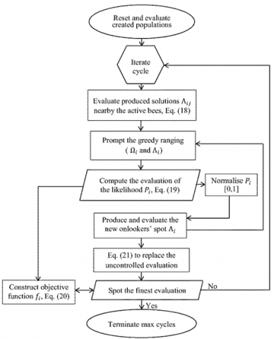
The ABC swarm intelligent optimizer procedure is broadly approached to penalize the design matrices in many large-scale applications nowadays. The ABC stages comprise initializing, employing bees, arranging onlooker bees and scouting bees. The quasi-ABC flowchart is shown in Figure 1. The attained populations are first reset and evaluated; the algorithm is then iterated for the first cycle and follows the diagram, and uses the provided equations to achieve the calculations. The algorithm will be terminated when the design objective is met. Furthermore, the iterations will be kept till the maximum cycles are reached or no adequate evaluation is found.
The produced solutions Λij nearby the employed bees can be evaluated by:
${{\Omega }_{ij}}{{\Lambda }_{ij}}={{\Omega }_{ij}}+{{\mu }_{ij}}\left( {{\Omega }_{ij}}-{{\Omega }_{kj}} \right)$ (18)
where, i, j and k are i, j and k-areas evaluating parameters, and μ is an arbitrary array around minus or plus one.
An evaluation of the likelihood Pi can be computed by:
${{P}_{i}}=\frac{{1}/{\left( 1+{{f}_{0}} \right)}\;}{\sum\nolimits_{i=1}^{N}{{1}/{\left( 1+{{f}_{i}} \right)}\;}}\,\,\,\,:\,\,\,{{f}_{i}}\ge 0$ (19)
where, N is several feasible solutions.
Figure 1. ABC algorithm illustration
The unique objective function fi maybe constructed by multi-objective optimization for certain objective functions [21].
${{f}_{i}}=\sum\nolimits_{i=1}^{n}{{{F}_{i}}{{O}_{i}}}$ (20)
where, Oi is the design objective requirements holding desired overshoot, settling criteria, and steady-state errors. Fi is the control limit residual.
The accessible abandoned evaluation has to be replaced with fresh ones Ωi for the lookout horizon.
${{\Omega }_{ij}}=\min {{\Omega }_{j}}+rand(0,1)\left( \max {{\Omega }_{j}}-\min {{\Omega }_{j}} \right)$ (21)
3.1 Uncontrolled lateral-directional characteristics
B747-100 lateral-directional uncontrolled flight was initially simulated at CI, CII, and CIII. This scenario mimics no pilot interference with the control mechanisms during stick-fixed flying. The plane was excited for unit step states, including 1° roll and yaw angles (the significant influence of altitude) and one m/sec resultant flight velocity (the primary influence of thrust). The linearized lateral-directional dynamics were modelled at those three trimmed flight conditions based on the A/C and stability derivatives [35] using Eq. (2). They can be summarized in Table 1. The B747-100 models of lateral-directional coupling variables were obtained with no aileron and rudder controls. Such itemizations gave ten TFs using Eq. (6) for lateral-directional variables at each Mach number and altitude case concerning the aileron and rudder inputs. The stability of lateral-directional motion can be evaluated by the eigenvalues of the A matrix or the characteristic equations given in Eq. (4). All those TFs had the same dominators. The coefficients of numerator TF aileron control off at three lateral-directional B747-100 flight cases are shown in Table 2.
Table 1. Uncontrolled B747-100 lateral characteristics
|
FCs |
A |
B |
|
CI |
$\left[\begin{array}{cccc}-0.09 & 0 & -67.36 & 9.81 \\ -0.02 & -0.97 & 0.331 & 0 \\ 0.003 & -0.16 & -0.219 & 0 \\ 0 & 1 & 0 & 0\end{array}\right]$ |
$\left[\begin{array}{cc}0 & 0.99 \\ -0.227 & -0.07 \\ -0.025 & -0.15 \\ 0 & 0\end{array}\right]$ |
|
CII |
$\left[\begin{array}{cccc}-0.08 & 0 & -157.9 & 9.81 \\ -0.001-0.65 & 0.378 & 0 \\ 0.003 & -0.07 & -0.142 & 0 \\ 0 & 1 & 0 & 0\end{array}\right]$ |
$\left[\begin{array}{cc}0 & 2.068 \\ -0.128 & 0.154 \\ -0.017 & -0.39 \\ 0 & 0\end{array}\right]$ |
|
CIII |
$\left[\begin{array}{cccc}-0.061 & 0 & -265.5 & 9.81 \\ -0.005 & -0.46 & 0.282 & 0 \\ 0.004 & -0.02 & -0.142 & 0 \\ 0 & 1 & 0 & 0\end{array}\right]$ |
$\left[\begin{array}{cc}0 & 1.233 \\ -0.19 & 0.106 \\ 0.01 & -0.44 \\ 0 & 0\end{array}\right]$ |
1. FCs (flight cases), 2. CI (M = 0.2, h = 0 m), 3. CII (M =0.5, h = 6096 m), 4. CIII (M = 0.9 and h = 12192 m)
Table 2. Numerator T.F. of aileron control off
|
FCs |
LSs |
a0 |
a1 |
a2 |
a3 |
|
CI |
v |
0.568 |
-3.027 |
-1.701 |
0 |
|
p |
0 |
-0.084 |
-0.078 |
-0.227 |
|
|
r |
-0.0107 |
0.001 |
0.01 |
-0.025 |
|
|
ϕ |
-0.079 |
-3.026 |
-0.227 |
0 |
|
|
β |
0.568 |
-3.026 |
-1.701 |
0 |
|
|
CII |
v |
-0.241 |
-0.847 |
2.69 |
0 |
|
p |
0 |
-0.062 |
-0.035 |
-0.128 |
|
|
r |
-0.004 |
0 |
-0.004 |
-0.017 |
|
|
ϕ |
-0.062 |
-0.035 |
-0.128 |
0 |
|
|
β |
-0.241 |
-0.847 |
2.69 |
0 |
|
|
CIII |
v |
-0.24 |
-3.595 |
-1.872 |
0 |
|
p |
0 |
-0.174 |
-0.036 |
-0.186 |
|
|
r |
-0.007 |
0.001 |
0.007 |
0.008 |
|
|
ϕ |
-0.174 |
-0.036 |
-0.186 |
0 |
|
|
β |
-0.24 |
-3.595 |
-1.872 |
0 |
LSs (lateral states)
The coefficients of numerator TF rudder control off at three lateral-directional B747-100 flight cases are shown in Table 3. The coefficients of denominator TF aileron and rudder control off at three lateral-directional B747-100 flight states are shown in Table 4. The characteristic equations are of the fourth order in the s Laplace variable. However, pole-zero cancellations at the origin may sometimes make the order less than a fourth. The eigenvalues show that lateral-directional dynamic motion consists of several oscillatory modes. Negative conjugate eigenvalues indicate the static stability of the airplane. However, a pair of eigenvalues was very close to the imaginary axis. One of them at the origin indicates that the plane may not sufficiently be dynamically stable to perform safe manoeuvring flight under the three conditions. The aircraft lateral-directional motion exhibited poor responses with high overshoot, long settling time and high oscillations. Aileron and rudder commands have to be controlled to enhance those responses. Prominent peaks in the oscillatory responses were found owing to the system zeroes’ effects on the underlying dynamics.
Table 3. Numerator TF of rudder control off
|
FCs |
LSs |
a0 |
a1 |
a2 |
a3 |
|
CI |
v |
-0.349 |
11.53 |
11.38 |
0.997 |
|
p |
0 |
-0.197 |
-0.049 |
0.066 |
|
|
r |
-0.028 |
0.008 |
-0.169 |
-0.151 |
|
|
ϕ |
-0.197 |
-0.049 |
0.066 |
0 |
|
|
β |
-0.349 |
11.53 |
11.38 |
0.997 |
|
|
CII |
v |
-1.239 |
43.63 |
63.49 |
2.068 |
|
p |
0 |
-0.038 |
-0.115 |
0.154 |
|
|
r |
0.003 |
-0.0173 |
-0.291 |
-0.392 |
|
|
ϕ |
0.038 |
-0.115 |
0.153 |
0 |
|
|
β |
-1.24 |
43.63 |
63.49 |
2.068 |
|
|
CIII |
v |
-1.074 |
55.58 |
118 |
1.231 |
|
p |
0 |
-0.492 |
-0.109 |
0.106 |
|
|
r |
-0.018 |
-0.010 |
-0.227 |
-0.442 |
|
|
ϕ |
-0.492 |
-0.109 |
0.106 |
0 |
|
|
β |
-1.074 |
55.58 |
118 |
1.231 |
Table 4. Denominator TF of aileron/rudder control off
|
FCs |
LSs |
b0 |
b1 |
b2 |
b3 |
b4 |
|
CI |
v p r ϕ |
0.03 |
0.60 |
0.55 |
1.3 |
1 |
|
β |
2.29 |
40.6 |
36.8 |
86 |
68 |
|
|
CII |
v p r ϕ |
-0.01 |
0.32 |
0.64 |
0.9 |
1 |
|
β |
-1.6 |
49.9 |
101 |
138 |
158 |
|
|
CIII |
v p r ϕ |
0 |
0.53 |
1.08 |
0.66 |
1 |
|
β |
-0.8 |
139.9 |
288 |
176 |
266 |
3.2 Controlled lateral-directional responses
The Q and H optimal matrices were reached with the ABC satisfying control requirements and good performance. In order to avoid the effects of sensitivity on the system control performance, the best solutions according to fitness were verified among 150 iterations of weighting attempts. Section 3.5 gives further discussions. The state vector had been utterly remodelled from the independent continuous measurement of w(t). The K gains of the H∞ algorithm revised the controlled state matrix AC as shown in Table 5. The stability of lateral-directional motion was re-evaluated by the eigenvalues of AC using Eq. (14) and Eq. (15). The characteristic equations are of the fourth order in the “s” Laplace variable. The eigenvalues of the lateral-directional uncontrolled flight modes have now been moved farther away from the imaginary axis into the left s-plane. Negative real eigenvalues were found in CI compared with negative conjugates in CII and CIII. The plane tends to be dynamically stable to perform manoeuvring flights under those conditions. Convergent responses are obtained for the three cases with no harmful oscillations and overshoots. The resultant lateral-directional variables concerning the coupling control ($\Delta \delta=\Delta \delta_a \cup \Delta \delta_r$) were compared in the three cases.
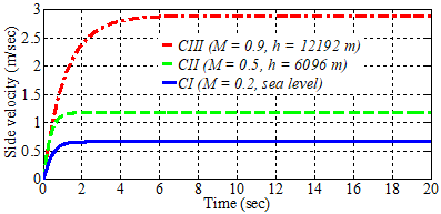
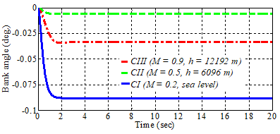
Figure 2 shows the side velocity responses $\left(\frac{v}{\Delta \delta}\right)$ of the three cases. The settling time is almost the same as two sec for both CI and CII. CIII took a more settling time of seven sec to reach the steady-state lateral flight. The side velocity got higher with increasing the forward velocity, which is the reason for the difference in the amplitudes. The H∞SAD produced well-converged flat responses with no overshoots. Figure 3 shows the bank “roll” angle responses ($\frac{\phi}{\Delta \delta}$) in the three cases. Both CI and CII almost had the same settling time of three secs. The steady-state is almost 4.3 sec for CIII. The steady-state amplitudes in CI, CII and CIII, are equal to -0.089°, -0.006° and -0.034°, respectively. The highest bankroll angle happened at a lower altitude and Mach number case, i.e., CI during the landing flight phase. However, the lowest bank angle occurred at M=0.5 and h=6096 m (CII). The roll subsidence convergence took a long time as the Mach number and altitude would get higher. Overall, the H∞SAD attenuated all visible forms of bank angle perturbations for the three cases.
Table 5. Controlled B747-100 lateral characteristics
|
FCs |
AC |
|
CI |
$\left[\begin{array}{cccc}-1.725 & -6.609 & -20.62 & -12.098 \\ -0.052 & -9.567 & 0.840 & -23.55 \\ 0.259 & -0.066 & -7.603 & 0.862 \\ 0 & 1 & 0 & 0\end{array}\right]$ |
|
CII |
$\left[\begin{array}{cccc}-3.562 & -9.909 & -54.952 & -41.815 \\ -0.225 & -7.485 & 5.722 & -21.52 \\ 0.667 & 0.996 & -19.94 & 7.419 \\ 0 & 1 & 0 & 0\end{array}\right]$ |
|
CIII |
$\left[\begin{array}{cccc}-0.417 & 0.145 & -141.599 & 8.323 \\ -0.035 & -3.460 & 10.532 & -6.025 \\ 0.131 & 0.043 & -44.567 & 0.765 \\ 0 & 1 & 0 & 0\end{array}\right]$ |
Figure 2. Side velocities of lateral controlled flight
Figure 3. Bank responses of lateral controlled flight
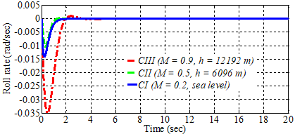
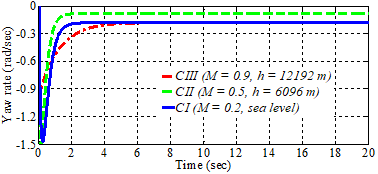
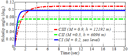
Figure 4 shows the roll rate responses ($\frac{p}{\Delta \delta}$) in the three cases. Large fluctuations found during the first seconds with a bit of overshoot, particularly in CIII. The overshot in CIII was a result of the roots of the spiral convergence mode, which are a little bit close to the imaginary axis. Quite similar roll rate responses are seen for CI and CII. The spiral model affects the time response of the three cases, which shows the lowest period of 0.281 sec in CI and the highest period in CIII of 1.176 sec. Overall the H∞SAD well excluded the roll disturbances in less than five secs within zero amplitude steady states. Figure 5 shows the responses to the yaw rate ($\frac{r}{\Delta \delta}$) in the three cases. The settling times were almost the same for CI and CII. CIII took a more settling time of 5.8 sec to reach the steady state. Both CI and CIII had almost the same yaw rate perturbations of -0.181 rad/sec. The Dutch roll mode spent more time on high Mach number and altitude cases than the low one. Figure 6 shows the responses of the sideslip angle ($\frac{\beta}{\Delta \delta}$) in the three cases. CI converged at the settling time of 2.2 sec with amplitude of 0.0974°. CII took a settling time of 1.85 sec with amplitude of 0.0742°, and CIII converged at the settling time of 6.05 sec with the highest amplitude of 0.109°. Overall, the H∞SAD attenuated perceptible sideslip perturbations for the three cases. Also, almost no opposite turn as the roll-yaw rotation rates incline toward being diminished due to the lateral coupling stick and rudder pedal rather than an un-modelled wind factor may typically hit the vertical tail.
Figure 4. Roll rates of lateral controlled flight
Figure 5. Yaw rates of lateral controlled flight
Figure 6. Sideslip responses of lateral controlled flight
3.3 Controlled lateral-directional modes
Once stably convergent lateral-directional flight was achieved under coupling unit step aileron-rudder of 1°, the reference input full-state feedback autopilot designs [34] were searched based on lateral velocity and bank angle for no roll and yaw. The side velocity was almost 30% of the total velocity. From Figure 2, the side velocities converged to sitting values based on a factor of 27.5 for the three cases. The numerator TF coefficients based on combined aileron and rudder control at three lateral-directional B747-100 flight cases are shown in Table 6.
Table 6. Numerator TF aileron and rudder control
|
FCs |
LSs |
a0 |
a1 |
a2 |
a3 |
|
CI |
v |
14,300 |
7,381 |
1,207 |
61.04 |
|
p |
0 |
35.67 |
24.63 |
3.842 |
|
|
r |
-7.129 |
-209.7 |
-88.16 |
-9.29 |
|
|
ϕ |
35.67 |
24.63 |
3.842 |
0 |
|
|
β |
14,300 |
7,381 |
1,207 |
61.04 |
|
|
CII |
v |
94,480 |
38,720 |
6,475 |
177 |
|
p |
0 |
309.2 |
131.2 |
15.82 |
|
|
r |
-20.96 |
-602.2 |
-225.1 |
-33.17 |
|
|
ϕ |
309.2 |
131.2 |
15.82 |
0 |
|
|
β |
94,480 |
38,720 |
6,475 |
177 |
|
|
CIII |
v |
29,560 |
17,320 |
5,090 |
51.32 |
|
p |
0 |
95.54 |
143.9 |
7.578 |
|
|
r |
-2.118 |
-109.2 |
-64.77 |
-18.53 |
|
|
ϕ |
95.54 |
143.9 |
7.578 |
0 |
|
|
β |
29,560 |
17,320 |
5,090 |
51.32 |
The denominator TF coefficients based on combined aileron and rudder control at three lateral-directional B747-100 flight states are shown in Table 7. The characteristic equations are of the fourth order in the s Laplace variable, where the eigenvalues show several lateral-directional flights of dynamic stability modes. The aircraft lateral-directional motion exhibited respectable responses with low overshoot, short settling time and minor oscillations. The flying quality is then checked for the three lateral-directional modes. Three well-known modes related to lateral-directional motion are already termed RS, SC and DR. These modes were recognized by the period and the damping ratio. Table 8 shows lateral-directional modes at the three flight conditions. The natural frequency, damping ratio and their product should generally exceed the minimum values of 0.4 rad/sec, 0.08 and 0.1 rad/sec, respectively, for the mode at the well-known Cooper-Harper scale [1, 35]. The DR modes are adequately damped for the three cases. However, the RS mode is relatively faster than the SC mode and is more pronounced at higher Mach number and altitude constraints.
Table 7. Denominator TF of aileron/rudder control
|
FCs |
LSs |
b0 |
b1 |
b2 |
b3 |
b4 |
|
CI |
v p r ϕ |
410.4 |
354.58 |
115.22 |
17.342 |
1 |
|
β |
27,646 |
23,884 |
7,761 |
1,168 |
67.36 |
|
|
CII |
v p r ϕ |
1,181 |
840.2 |
231.7 |
28.55 |
1 |
|
β |
186,500 |
132,700 |
36,580 |
4,507 |
157.9 |
|
|
CIII |
v p r ϕ |
219 |
391.9 |
198.5 |
48.45 |
1 |
|
β |
58,130 |
104,000 |
52,690 |
12,860 |
265.5 |
Table 8. B747-100 lateral-directional modes
|
FCs |
LMs |
λ |
ξ |
Frequency (rad/sec) |
Period (sec) |
|
CI |
RS |
-6.58 |
1.00 |
6.58 |
0.151 |
|
SC |
-2.86 |
1.00 |
2.86 |
0.349 |
|
|
DR |
-3.95±2.49i |
0.846 |
4.67 |
0.214 |
|
|
CII |
RS |
-18.1 |
1.00 |
18.1 |
0.055 |
|
SC |
-3.55 |
1.00 |
3.55 |
0.281 |
|
|
DR |
-3.44±2.56i |
0.802 |
4.29 |
0.233 |
|
|
CIII |
RS |
-44.14 |
1.00 |
44.1 |
0.022 |
|
SC |
-0.851 |
1.00 |
0.850 |
1.176 |
|
|
DR |
-1.72±1.69i |
0.714 |
2.42 |
0.413 |
LMs (lateral modes)
3.4 Flying quality assessments
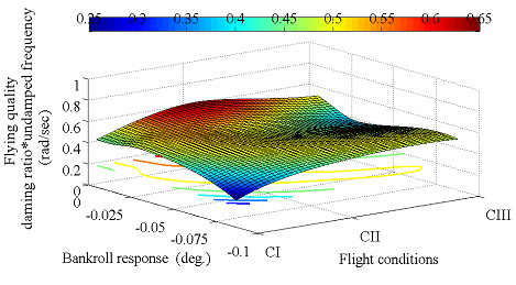
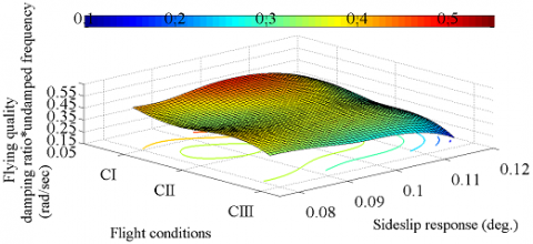
Figure 7. DR flying qualities of bankrolling control
Figure 8. DR flying qualities of sideslipping control
The flying quality properties for the DR mode of B747-100 lateral controlled flight based on bankroll and sideslip responses are assessed in Figures 3 and 6. The federal aviation (FARs) or military specifications (MILSPECs) regulate permissible flying stability requirements [36]. These flying qualities are evaluated based on the level I mission flight phase [1, 35] for the product of damping ratio and undamped natural frequency (ξωd) of the DR mode, namely, ξ×ωd≥0.1 rad/sec [1, 36]. Moreover, ξ≥0.08 and ωd≥0.4 rad/sec [35] were also widely verified. The DR lateral oscillation represents flat yaw and sideslip under no roll. The DR mode is similar to a short period of longitudinal flight [35]. Figure 7 shows DR flying qualities for B747-100 lateral-directional bank-rolling controlled flight. The 3D surface represents ξωd the vertical axis, the bankroll ϕ alongside the cross-horizontal axis and the flight cases alongside the horizontal axis. The minimum flying qualities are based on ξωd were overall met for the ϕ responses as high as 0.265 rad/sec. Figure 8 shows DR flying qualities for B747-100 lateral-directional sideslipping controlled flight. The 3D surface represents ξωd alongside the vertical axis, sideslip β alongside the cross-horizontal axis and the flight cases alongside the horizontal axis. The minimum flying qualities based on ξωd were overall met for the β responses as most values exceed 0.137 rad/sec.
The tolerable skidding turn has to fall within $1 \leq \frac{\left(\frac{\beta}{\phi}\right)}{\Delta \delta} \leq 15$ of the constricted turn radius in compliance with the airworthiness (authorities’) requirements [36]. Table 9 compare the B747-100 sideslip turn of three cases of steady-state responsiveness shown in Figures 3 and 6. All the lateral scenarios meet tolerable turn sideslip constraints, and the CI at sea level is more susceptible to sideslip turn effects due to the downward ground interaction. The sideslip response is also compared with flight testing from aircraft certification [36]. It shows satisfactory dampness in the sideslip incident by the tendency to raise the low wing with the aileron and rudder controls.
Table 9. B747-100 sideslip turn comparison
|
FCs |
β(º) |
ϕ (º) |
((β/ϕ))/Δδ |
|
CI |
0.0974 |
0.0862 |
1.1309 |
|
CII |
0.0737 |
0.0063 |
11.692 |
|
CIII |
0.1162 |
0.0326 |
3.565 |
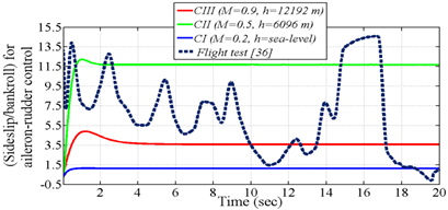
For benchmarking the sideslip dampening responsiveness, Figure 9 qualitatively compares the sideslip response obtained by the H∞-ABC synthesis and typical DR manoeuvre flight-time histories of sideslip control effectiveness [36]. It indicated that the DR mode of the test aircraft was achieved by first commanding the aileron stick, and then the rudder pedals were pushed. The response settled in 5-10 sec for the DR flight test lasted 15-20 sec [36]. A skidding turn was manageable by keeping a constant heading through the aileron stick followed by the rudder pedal to maintain the heading angle constant with low side speed deviation (shown in Figure 2). It did not indicate relative roll oscillations concerning the sideslip practice. The flying qualities airworthiness requirement stated that β≤3° for level I flight [36]. No disrupted skid is recognized as the flight test showed an almost minimal steady levelled responsiveness. It looks like the promising implementation of the H∞-ABC stability augmentation strategy to take place in the classical control system of tested aircraft. Flight tests based on steady heading sideslip manoeuvre [36] exhibited measured perturbations in sideslip-to-bankroll from 14.625 to 1.479 within the flight envelope ranging from CIII to CI cases studied here.
Figure 9. DR sideslip responsiveness validation
3.5 Sensitivity assessments
The steady-state step responsiveness fulfilling $O_3=\lim _{t \rightarrow \infty}\left[\begin{array}{lllll}v & p & r & \beta & \phi\end{array}\right]^T=-A_C^{-1} B_C \delta$ must die out for sideslip and bankroll perturbations of the coupling control inputs to assure the dynamic stability of the aircraft. Therefore, ABC factors were set between 0.1 and 150, the inhabitant dimension was taken at 15, and the total cycle did not exceed 200. Employed bee matrices were initially chosen diagonal. The ABC maximum generations were fixed to 2000, and the search space was imposed as 13×10×2000; 5×5×2000; 4×5×2000 which copes with the design spaces matrices. The coefficient settings, colony dimension and total cycles of the ABC optimization procedure were implemented between 0.12 and 60, 15 and 100, respectively. The algorithm was exacted for 25 runtimes on each benchmark case. Beginning with the most achievable criteria and then gradually adding one-by-one constraints until the most control merits were achieved with a low level of sensitivity to parameter variations associated with the weighting process of design matrices. The finest design matrices from the ABC optimizer only proceeded for trade-offs amongst the overshot, settling epoch, the steady-state errors, the convergence and the computation effort. The accuracy of the H∞ and ABC approach was qualitatively measured by root mean square error and absolute error metrics [21, 23]. The precision of the ABC optimizer in the estimations of the H∞ weighting matrices regresses as high as 88% for the most lateral manoeuvre responses achieved.
The ABC parameters used for the lateral states are shown in Table 10. Those were supportive of minimizing the cost function (fi, i=1:3) in Eq. (20) and thus obtaining the optimal weighting matrices. A demo is next given for the v state variable, which is relevant to all the other state variables in Table 10. A satisfactorily v response was reached using the ABC algorithm constraints (O1<2% for desired overshoot, O2<7% required settling time, and O3<±1.7% the desired steady-state error). They had to be away from s=0, avoiding the ABC failure and H∞ destabilization. Fitness residuals of F1=0.6, F2=0.4, and F3=0.8 had been deployed to achieve reasonably optimized H∞ design matrices to augment the v response of lateral flight. As shown in Figure 2, all constraints are satisfied for three flight conditions at CI, CII and CIII. The maximum settling time reached 6.45 sec for M=0.9 and h=12192 m (CIII), with negligible overshoot and steady-state error.
Table 11 quantitatively compares objective functions. The standard deviation, best, averaged and worst results are compared with TER [34]. The ABC algorithm converges much better than without systematic optimization of the TER. Moreover, the obtained flight responses had reasonable convergences based on the ABC limitations tabulated in Table 10.
Table 10. ABC sensitivity
|
LSs |
Constraints |
Fitness |
||||
|
O1 |
O2 |
O3 |
F1 |
F2 |
F3 |
|
|
v |
2 |
7 |
1.7 |
0.6 |
0.4 |
0.8 |
|
p |
1.8 |
5 |
1.4 |
0.5 |
0.7 |
0.6 |
|
r |
1.6 |
4 |
1.8 |
0.6 |
0.7 |
0.9 |
|
ϕ |
1.1 |
4 |
1.3 |
0.8 |
0.7 |
0.6 |
|
β |
1.1 |
6 |
1.5 |
0.7 |
0.6 |
0.7 |
Table 11. ABC cost functions’ accuracy
|
CF |
Optimizer |
WS |
BS |
AS |
SD |
|
f1 |
TER [33] |
1.18E-02 |
1.24E-3 |
1.73E-02 |
1.43E-02 |
|
ABC |
1.67E-03 |
1.35E-6 |
1.87E-05 |
1.31E-05 |
|
|
f2 |
TER [33] |
3.76E-02 |
4.47E-3 |
1.07E-2 |
2.48E-2 |
|
ABC |
4.48E-04 |
3.86E-7 |
3.60E-6 |
7.72E-5 |
|
|
f3 |
TER [33] |
1.93E-02 |
2.57E-3 |
4.62E-3 |
2.48E-2 |
|
ABC |
1.25E-04 |
8.97E-6 |
3.76E-5 |
3.91E-4 |
1. CF (cost function); 2. WS (worst solution); 3. BS (best solution); 4. AS (averaged solution); 4. SD (standard deviation); 5. TER (trial and error rules)
The lateral flight modes significantly vary as the stability derivatives do with Mach number and altitude. Those modes normally behave at lower altitudes and have asymmetrical dampness at higher altitudes and Mach number. When substantial aeroelasticity and compressibility effects are added, more irregular lateral modes could be experienced. Additional freedom is admitted in guaranteeing the output feedback control quadratic performance concerning roll and yaw disturbances during the lateral-directional B747-100 flight. The H∞SAD control design tasks, which are solvable numerical problems, sufficiently opt for the Lyapunov stability of the closed-loop aircraft design. It minimizes the closed-loop lateral flight responses of bankroll and sideslip perturbations. An ABC optimizer gives robust performance and stabilization of those lateral characteristics like the well-known loop-shaping approach [4, 37]. There is no guarantee that such synthesis behaves well for the proper plant encountered in practice as did here for the nominal plant design. Many other flight disruptions may encounter causing sideslip and bankroll perturbations such as wind, faulty stabilizer and engine inoperative not being included here. An adequate response may be essential as the H∞ and ABC synthesis is flexible enough to handle add-on flight conditions. The ABC algorithm collaborates well to ensure the H∞SAD robust performance and consequently augment the stability and robustness. The Dutch roll modes reasonably meet (damping ratio × damping ratio × undamped frequency) flying qualities for the flight cases studied. The effectiveness of the controllers is pronounced for a safe recovery to routine flight from perturbed lateral conditions, particularly sideslip and roll bank disturbance attenuations. However, the flying quality of roll convergence and spiral modes may be further enhanced. Overall, 3D response surfaces, which signify trade-off patterns of the DR-mode flying quality versus the bankroll or sideslip free-disturbance responses and the flight conditions, indicate the minimum merits of flying qualities (ξ×ωd ≥ 0.1 rad/sec) for wide flight missions met [35].
As might be noticed, peak transitional behaviours were produced for the yaw rate and roll rate responses, further identifications of whether the nature of the H∞ method or the ABC algorithm or even the complete synthesis is behind such biased responses. Fortunately, these temporary behaviours quickly died out, and nominal roll and yaw rates were produced for three flight cases. Furthermore, stable, robust performance could also be analyzed using the gain scheduling or μ-control approaches through the whole lateral flight envelope. The YK parametrization might also be used to meet add-on criteria of un-modelled aircraft dynamics.
Thanks to the Mobility and Transport Research Centre (MTRC), Coventry University, the UK, for valuable supportive consultations. The University of Tripoli supports this research.
|
a0 |
transfer function numerator coefficient of s0 term |
|
a1 |
transfer function numerator coefficient of s term |
|
a2 |
transfer function numerator coefficient of s2 term |
|
a3 |
transfer function numerator coefficient of s3 term |
|
A |
aircraft system matrix |
|
ABC |
Artificial bee colony |
|
AC |
controlled aircraft matrix |
|
A/C |
aircraft |
|
b0 |
transfer function denominator coefficient of s0 term |
|
b1 |
transfer function denominator coefficient of s term |
|
b2 |
transfer function denominator coefficient of s2 term |
|
b3 |
transfer function denominator coefficient of s3 term |
|
b4 |
transfer function denominator coefficient of s4 term |
|
B |
aircraft stability derivative matrix |
|
C |
output observation matrix |
|
D |
state transition matrix |
|
DR |
Dutch roll oscillatory mode |
|
e |
the eigenvalue of spiral convergence mode |
|
f |
eigenvalues of rolling subsidence mode |
|
f0 |
baseline objective function |
|
fi |
unique objective function |
|
Fi |
control limit residual for design variables |
|
g |
gravity acceleration, m.sec-2 |
|
GA |
genetic algorithm |
|
h |
altitude, m |
|
H |
systematic matrix |
|
H∞ |
H-infinity |
|
H∞SAD |
H-infinity stability augmentation design |
|
ICQ |
inequality matrix of CQ dimension |
|
IS |
inequality matrix of S dimension |
|
${{{I}'}_{x}}$ |
the reformed moment around the x-axis, kg.m2 |
|
${{{I}'}_{z}}$ |
the reformed moment around the z-axis, kg.m2 |
|
${{{I}'}_{zx}}$ |
x-z symmetry plane moment inertia product, kg.m2 |
|
$\overset{\scriptscriptstyle\smile}{J}$ |
first design matrix of 4 by 4 size |
|
$K$ |
real matrix dynamics |
|
$\overset{\scriptscriptstyle\smile}{L}$ |
second design matrix of 4 by 4 size |
|
${{L}_{p}}$ |
roll moment derivative with respect to roll rate, kg.m2/sec/rad |
|
${{L}_{r}}$ |
roll moment derivative with respect to yaw rate, kg.m2/sec/rad |
|
${{L}_{v}}$ |
roll moment derivative with respect to side velocity, kg.m2/sec/rad |
|
LQR |
linear quadratic regulator |
|
LQG |
linear quadratic Gaussian |
|
$m$ |
aircraft mass, kg |
|
M |
Mach number, dimensionless |
|
$\overset{\scriptscriptstyle\smile}{M}$ |
third design matrix of 2 by 4 size |
|
$n$ |
the upper limit of search space |
|
$\overset{\scriptscriptstyle\smile}{N}$ |
forth design matrix of 2 by 4 size |
|
N |
likely solutions number |
|
${{N}_{p}}$ |
yaw moment derivative with respect to roll rate, kg.m2/sec/rad |
|
${{N}_{r}}$ |
yaw moment derivative with respect to yaw rate, kg.m2/sec/rad |
|
${{N}_{v}}$ |
yaw moment derivative with respect to side velocity, kg.m2/sec/rad |
|
${{O}_{i}}$ |
design objectives |
|
$p$ |
rolling rate, rad.sec-1 |
|
${{P}_{i}}$ |
likelihood function |
|
PID |
proportional-integral-derivative |
|
$q$ |
controller variable vector |
|
${{q}_{1}}$ |
first controller variable |
|
${{q}_{2}}$ |
second controller variable |
|
${{q}_{3}}$ |
third controller variable |
|
${{q}_{4}}$ |
fourth controller variable |
|
$Q$ |
positive definite symmetric matrix |
|
$r$ |
yawing rate, rad.sec-1 |
|
RS |
rolling subsidence mode |
|
s |
Laplace variable |
|
SAD |
stability augmentation design |
|
SC |
spiral convergence mode |
|
TER |
trail and error rule |
|
TF |
transfer function |
|
${{u}_{0}}$ |
steady-state velocity, m.sec-1 |
|
$u\left( t \right)$ |
control law |
|
$v$ |
side velocity, m.sec-1 |
|
$V$ |
aircraft velocity, m.sec-1 |
|
$w\left( t \right)$ |
preferred response signal vector |
|
$W$ |
static decoupling signal gain matrix |
|
$Y$ |
output matrix |
|
${{Y}_{p}}$ |
normal force derivative with respect to roll rate, kg.m/sec/rad |
|
${{Y}_{r}}$ |
normal force derivative with respect to yaw rate, kg.m/sec/rad |
|
${{Y}_{v}}$ |
normal force derivative with respect to side velocity, kg.m/sec/rad |
|
Greek symbols |
|
|
$\beta $ |
sideslip angle, rad, deg. |
|
$\gamma $ |
positive scalar |
|
${{\delta }_{a}}$ |
aileron control action |
|
${{\delta }_{r}}$ |
rudder control action |
|
$\Delta $ |
perturbation |
|
$\varepsilon $ |
dynamic disturbance parameter |
|
${{\theta }_{0}}$ |
reference trim angle, rad, deg. |
|
$\lambda $ |
eigenvalue, dimensionless |
|
${{\Lambda }_{ij}}$ |
solutions nearby the employed bees |
|
$\mu $ |
arbitrary array |
|
$\xi $ |
damping coefficient, dimensionless |
|
$\sigma $ |
control energy parameter |
|
$\phi $ |
bankroll angle, rad, deg. |
|
${{\omega }_{d}}$ |
undamped natural frequency, rad.sec-1 |
|
${{\Omega }_{j}}$ |
fresh abandoned evaluation of j element |
|
${{\Omega }_{ij}}$ |
abandoned evaluation of $ij$ neighbour |
|
${{\Omega }_{kj}}$ |
abandoned evaluation of $kj$ neighbour |
|
Subscripts |
|
|
0 |
steady-state |
|
$i$ |
i-area evaluating parameter |
|
$j$ |
j-area evaluating parameter |
|
$k$ |
k-area evaluating parameter |
|
$c$ |
derivatives with respect to ${{\delta }_{a}}$ and ${{\delta }_{r}}$ |
|
$p$ |
rolling rate |
|
$r$ |
yawing rate |
|
$v$ |
side velocity |
[1] Mclean, D. (1990). Automatic Flight Control Systems, UK. The Prentice-Hall International. http://dx.doi.org/10.1177/002029400303600602
[2] Blight, J.D., Gangsaas, D., Richardson, T.M. (1986). Control law synthesis for an airplane with relaxed static stability. Journal of Guidance, Control, and Dynamics, 9(5): 546-554. http://dx.doi.org/10.2514/3.20145
[3] Shiau, J.K., Ma, DM (2009). An autopilot design for the longitudinal dynamics of a low-speed experimental UAV using two-time-scale cascade decomposition. Transactions of the Canadian Society for Mechanical Engineering, 33(3): 501-521. https://doi.org/10.1139/tcsme-2009-0034
[4] Shinners, S.M. (1998). Modern Control System Theory and Design, Wiley Inter-Science. http://dx.doi.org/10.1016/0005-1098(93)90034-q
[5] Tosun, D.C., Işık, Y., Korul, H. (2015). LQR control of a quadrotor helicopter. New Developments in Pure and Applied Mathematics, pp. 247-252. http://dx.doi.org/978-1-61804-287-3
[6] Joukhadar, A., Hasan, I., Alsabbagh, A., Kouzbary, M. (2015). Integral LQR-based 6DOF autonomous quadrocopter balancing system control. International Journal of Advanced Research in Artificial Intelligence, 4(5). http://dx.doi.org/10.14569/IJARAI.2015.040502
[7] Shaji, J., Aswin, RB (2015). Pitch control of aircraft using LQR & LQG control. International Journal of Advanced Research in Electrical, Electronics and Instrumentation Engineering, 4(8): 6981-6987. http://dx.doi.org/10.15662/ijareeie.2015.0408033
[8] Adîr, V.G., Stoica, A.M. (2012). Integral LQR control of a star-shaped octorotor. Incas Bulletin, 4(2): 3-18. http://dx.doi.org/10.13111/2066-8201.2012.4.2.1
[9] Tayebi, J., Nikkhah, A., Roshanian, J. (2017). LQR/LQG attitude stabilization of an agile microsatellite with CMG. Aircraft Engineering and Aerospace Technology, 89(2): 290-296. http://dx.doi.org/10.1108/AEAT-07-2014-0102
[10] Hajiye, C., Soken, H.E., Vural, S.Y. (2015). State estimation and control for low-cost unmanned aerial vehicles. Springer International Publishing. Switzerland, pp. 176-200. http://dx.doi.org/10.1007/978-3-319-16417-5
[11] Darwish, M.H., Elgohary, A.A. Gomaa, M.M. Kaoud, A.M. Ashry, A.M., Taha., HE (2022). A comparative assessment of the performance of PID and MPC controllers: A UAV altitude hold autopilot case study, AIAA SCITECH 2022 Forum. https://doi.org/10.2514/6.2022-1519
[12] Bharathi, M., Kumar, G. (2013). An LQR controller design approach for pitch axis stabilization of 3-DOF helicopter system. International Journal of Scientific & Engineering Research, 4(4).
[13] Oner, K.T., Cetinsoy, E., Sirimoglu, E., Hancer, C., Ayken, T., Unel, M. (2009). LQR and SMC stabilization of a new unmanned aerial vehicle. International Journal of Aerospace and Mechanical Engineering, 3(10): 1190-1195. https://publications.waset.org/pdf/2009.
[14] Sareban, M. (2017). Evaluation of three common algorithms for structure active control. Engineering, Technology & Applied Science Research, 7(3): 1638-1646. https://doi.org/10.5281/zenodo.1056268
[15] Aktas, K.G., Esen, I. (2020). State-space modeling and active vibration control of smart flexible cantilever beam with the use of finite element method. Engineering Technology & Applied Science Research, 10(6): 6549-6556. https://doi.org/10.48084/etasr.3949
[16] Sharma, V., Voulgaris, P.G., Frazzoli, E. (2004). Aircraft autopilot analysis and envelope protection for operation under icing condition. Journal of Guidance Navigation, and Control, 27(3): 454-465. https://arc.aiaa.org/doi/abs/10.2514/1.12144100
[17] Lungu, R., Lungu, M. (2014). Automatic landing control using H-inf control and dynamic inversion. Proceedings of the Institution of Mechanical Engineers. Part G: Journal of Aerospace Engineering, 228(14): 2612-2626. https://doi.org/10.1177/0954410014523576
[18] Li, S.E., Gao, F., Li, K., Wang, L., You K., Cao, K. (2018). Robust longitudinal control of multi-vehicle systems-A distributed H-infinity method. IEEE Transactions on Intelligent Transportation Systems, 19(9): 2779-2788. http://dx.doi.org/10.1109/TITS.2017.2760910
[19] Rigatos, G., Siano, P.A. (2015). New nonlinear H-infinity feedback control approach to the problem of autonomous robot navigation. Intelligent Industrial Systems, 1, pp. 179-186. http://dx.doi.org/10.1007/s40903-015-0021-x
[20] Giacomán-Zarzar, M., Ramirez-Mendoza, R., Fleming, P.J., Griffin, I., Molina-Cristóbal, A. (2008). Robust H∞ controller design for aircraft lateral dynamics using multi-objective optimization and genetic algorithms. Proceedings of the 17th World Congress the International Federation of Automatic Control, Seoul. Korea. http://dx.doi.org/10.3182/20080706-5-kr-1001.01493
[21] Karaboga, D., Basturk, B. (2008). On the performance of artificial bee colony algorithm. Applied Soft Computing, 8(1): 687-697. https://doi.org/10.1016/j.asoc.2007.05.007
[22] Ata, B., Coban, R. (2014). Artificial bee colony algorithm based linear-quadratic optimal controller design for a nonlinear inverted pendulum. International Journal of Intelligent Systems and Applications in Engineering, 3(1): 1-6. http://dx.doi.org/10.18201/ijisae.87020
[23] Karaboga, D., Akay, B. (2009). A comparative study of artificial bee colony algorithm. Applied Mathematics and Computation, 214(1): 108-132. https://doi.org/10.1016/j.amc.2009.03.09
[24] Marouani, Ι., Boudjemline, A., Guesmi, T., Abdallah, H.H. (2018). A modified artificial bee colony for the non-smooth dynamic economic/environmental dispatch. Engineering, Technology & Applied Science Research, 8(5): 3321-3328. https://doi.org/10.48084/etasr.2098
[25] Alshammari, G.A., Alshammari, F.A., Guesmi, T., Alshammari, B.M., Alshammari, A.S., Alshammari, N.A. (2021). A new particle swarm optimization based strategy for the economic emission dispatch problem including wind energy sources. Engineering, Technology & Applied Science Research, 11(5): 7585-7590. https://doi.org/10.48084/etasr.4279
[26] Al-awad, N.A. (2020). Optimal controller design for reduced-order model of rotational mechanical system. Mathematical Modelling of Engineering Problems, 7(3): 395-402. https://doi.org/10.18280/mmep.070309
[27] Belletti, J.P.A., Zavoli, A. Trotta, D., Matteis. GD (2021). Advanced H-infinity synthesis for launch vehicle attitude control in atmospheric flight. AIAA SciTech 2021. https://doi.org/10.2514/6.2021-1217
[28] Hamza, A., Mohamed A.H., El-Badawy, A. (2022). Robust H-infinity control for a quadrotor UAV. AIAA SCITECH 2022 Forum. https://doi.org/10.2514/6.2022-2033
[29] Rachyd, H., Mulder, M., Veld A., Paassen, R. (2006). Design and evaluation of a pilot support system for lateral three-degree decelerating approaches. AIAA Guidance, Navigation, and Control Conference and Exhibit. Keystone, Colorado. https://doi.org/10.2514/6.2006-6063
[30] Klyde, D.H., Lampton A.K., Schulze. PC (2017). Evaluation of a steep turn spatial disorientation demonstration scenario for commercial pilot training. AIAA Modeling and Simulation Technologies Conference. Grapevine, Texas, https://doi.org/10.2514/6.2017-1079
[31] Tian, P., Chao, H. (2018). Model aided estimation of angle of attack, sideslip angle, and 3d wind without flow angle measurements. AIAA Guidance, Navigation, and Control Conference. https://doi.org/10.2514/6.2018-1844
[32] Silva, O.R., Nunes, C.D., Hayashi, M.T., Neves., GF (2022). Investigation of propeller slipstream effects on the lateral directional stability and control sizing of a light twin engine aircraft. AIAA SCITECH 2022 Forum. https://doi.org/10.2514/6.2022-0689
[33] Jouda MS, Kahraman N. (2022). Improved optimal control of transient power sharing in microgrid using H-infinity controller with artificial bee colony algorithm. Energies, 15(3): 1043. http://dx.doi.org/10.3390/en15031043
[34] Elarbi, E.M., Laila, D.S., Ghmmam, A.A., Horri, N.M. (2017). LQR reference tracking control of Boeing 747-100 longitudinal dynamics with CG shifts. 6th International Conference on Advanced Technology and Sciences 17, Riga. Latvia. SN Bilgi Teknolojileri. http://dx.doi.org/10.12080/icat2017-358019
[35] Etkins, B. (1994). Dynamics of flight: Stability and control. Physics Today, 12(9): 54. http://doi.org/10.1063/1.3060977
[36] Jitendra, R., Jatinder, S. (2009). Flight Mechanics Modeling and Analysis. Taylor & Francis Group, LLC. http://doi.org/10.1201/b15919
[37] Gu, D.W, Petkov, P.H., Konstantinov, M.M. (2005). Robust Control Design with Matlab, Springer-Verlag London Limited. http://doi.org/10.1007/978-1-4471-4682-7