Juan Gabriel Rueda-Bayona* | Natalia Paez | Juan José Cabello Eras | Alexis Sagastume Gutiérrez
© 2022 IIETA. This article is published by IIETA and is licensed under the CC BY 4.0 license (http://creativecommons.org/licenses/by/4.0/).
OPEN ACCESS
The need of reducing the dependence of fossil fuels and CO2 emissions have motivated the diversification of energy matrix. Among the Renewables, the hydropower shows better characteristics compared to solar, wind, biomass and geothermal, because its low CO2 emissions, higher density and others technical factors. Within the Hydropower, the Hydrokinetic turbines (HT) are considered as a promising technology because can provide electricity during low flow velocity conditions (< 2 m/s) and is able to operate in shallow waters < 8 m and in secluded areas without access to the energy network. In this sense, the present study incentivizes the research in Hydropower and proposes and new application of DOE-ANOVA combined with Computational Fluid Dynamics (CFD) modelling for the HT design and optimization. Accordingly, this work evaluated the performance of a HT with 1.9 m of rotor diameter operating in a water flow of 1.5 m/s through a 23 factorial design with 9 modelling cases (MC). The results showed that the increment of outlet diameters increased the downstream velocity and the hydrodynamic pressure over the HT, and the reduction of the blade tip edge distance generated an increment of the response of the HT hydraulic and mechanical properties.
CFD, DOE-ANOVA, hydrokinetic microturbine, multiple regression, optimization
The rapid increase in human population, industries and the modernization of lifestyles, has increased the demand for fossil fuels to support the generation of electricity. Climate Change, the main global environmental concern, is closely related with the emissions of greenhouse gases (GHG), which have motivated international agreements to mitigate GHG emissions. Initiatives like the United Nations sustainable development goals (SDGs), aims to promote the access to clean and sustainable energy (Renewables) motivating strategies to mitigate the impacts of climate change. Currently, countries like China, the United States and the European Union are leading the transition to Renewables [1, 2]. The global electricity demand increased 75% between 2000 and 2018, from 13,152 TWh to 23,031 TWh, and it is estimated increase by 58% in the next 20 years [3].
That growing demand for electricity could be supported with Renewable energies (RE), with hydropower systems rising as an attractive choice because of its low emissions of GHGs (41 gCO2eq./KWh) contrasted to wind (80 gCO2eq./KWh) and solar (90 gCO2eq./KWh) technologies [4]. Hydropower systems can be exploited with traditional large scale plants with large dams [5], or using hydrokinetic turbines at a smaller scale alongside natural stream flows to take advantage of the kinetic energy from the current for power generation [6]. Hydrokinetic turbines, have been applied on river, tidal and ocean currents [7]. As compared to other renewable sources like Onshore and Offshore wind, Solar, Biomass, and Geothermal, Hydropower has advantages on the energy density, predictability of power production, capacity factor, GHG emissions, visual impact and generation costs [8]. The use of non-conventional renewable technologies, including solar, wind, biomass and small hydropower can help to address the need to provide clean energy to remote locations [9,10], and to communities with access to a low-quality and expensive electricity [11].
The HT are classified according the angle between the inflow vector and the plane of swept area (i.e axial flow, cross flow) [12] and the type of hydrokinetics (i.e river, tidal, oceanic) [13]. Nago et al. [13] performed a literature review and listed several inlet diameters (D) and operation velocities of HT, and we group them in micro (0.15 m < D < 0.7 m), mid (0.7 m < D <2 m) and large (D > 2 m), which may operate during low (< 1.5 m/s) or rapid velocity conditions (> 1.5 m/s).
Particularly, hydrokinetic turbines can be instrumental because they can operate at low flow velocity conditions (i.e. 0.3 to 0.7 m/s) requiring small infrastructure and low energy concentration [14]. Hydrokinetic turbines (HT) with swept diameters lower than 1 m are limited to shallow waters constraining power generation to few hundred watts under these conditions [15]. Therefore, HT must be grouped and configured in arrays to generate sufficient electricity for commercial developments [14], hence, optimizing this technology is cornerstone to make it feasible and accessible.
The research and development of HT have shown some progress recently with pilot projects and research studies using physical models and numerical modelling [16, 17]. Studies of HT for low velocity conditions have been performed for different applications like hydropower systems in irrigation channels [18], waterwheels and transverse horizontal axis turbines for moderate sized rivers [19] with ultra-low head turbines [15]. The interest in HT for tidal energy has materialized initiatives such as the Roosevelt Island Tidal Energy (RITE) project in the United States (New York) which utilized 30 HT in an array to produce 35 kW [20, 21]. In Canada the Maine project used 15 HT of 500 kW to provide electricity for the urban area of east Maine [22]. Other countries are identifying potential areas for tidal HT [11] and evaluating factors for the building and installation of new HT plants [23].
The design of HT starts with the shape definition, sizing and preliminary characterization of the model [24], and the concept evaluation through physical and numerical approaches such as the Computational Fluid Dynamics (CFD) simulations [25, 26]. Authors like Saini and Saini [27] performed physical and numerical simulations (CFD) using a model of a HT developed in ANSYS (www.ansys.com) to evaluate its performance under several experimental conditions; ANSYS is a multiphysics model capable of solving complex fluid-structure interactions [28]. The results show that hybrid rotor experienced smooth flow and low pressure over the structure. Ramadan et al. [29] assessed two Savonious rotor profiles within an irrigation channel through CFD modelling (ANSYS) and physical models. The research concluded that the FLUENT module of ANSYS model depicted an acceptable accuracy due to the numerical-experimental results.
The scour around submerged structures such as HT is considered critical for their stability. In this sense, Khaled et al. [30] implemented a CFD model in OpenFOAM (www.openfoam.com), to analyze the sediment transport around a hydrokinetic turbine. The study pointed that the energy extracted by the turbine altered the hydrodynamic field, which triggered scour phenomena and sediment deposition zones nearby the structure. Lee et al. [31] analyzed the axial flow of a 3D printed HT at several tip speed ratios and recommended new research for validating the experimental results through numerical modelling and a future optimization of the model through parameterized equations.
The optimization processes of HT for low velocity conditions have been carried out through the combination of CFD modelling and experimental data, analyzing the performance of the model at different scenarios considering the expertise of the researchers [32, 33]. Madav [34] performed CFD modelling (ANSYS) and experimental test to optimize a V-shaped hydrokinetic turbine for operating under a low velocity regime (i.e. 0.513 m/s), and pointed the effect of changing the aspect ratio increased the energy conversion. Espina-Valdés et al. [35] used experimental data and CFD modelling (ANSYS) to evaluate the effect of water pressure and velocity over a HT, and pointed as future work the improvement of CFD results when increasing the number of rotor blades. Tovar et al. [36] evaluated a HT through CFD modeling (ANSYS), and recommended specific materials for manufacturing the turbine, such as T84 aluminum because of its good mechanical properties against abrasive environments seen in the ocean environment.
The use of heuristics and artificial intelligence for optimizing turbines is evidenced in several studies, such as the application of Differential Evolution Algorithm (DEA) to improve the performance of blade sections [37]. Cavalari Labigalini et al. [38] configured a hybrid metaheuristic multi-objective optimization method to improve the performance of a hydrokinetic turbine; the study combined the methods Artificial Bee Colony (ABC), Simulated Annealing (SA), Particle Swarm Optimization (PSO) and the Flower Pollination Algorithm (FPA). As future research the study recommended CFD simulations and prototyping to validate the numerical results of the developed hybrid model. Other studies such as the performed by Bouvant et al. [39] have considered the Design of Experiment theory [40], and have used central composite design of experiments (CCD-DOE) and the surface response method to analyze the turbine model and to construct parameterized equations through second-order regression models for the optimization process.
Hydrokinetic turbines, considered a non-conventional technology, is costly and have low availability in the market. Additionally, the output power of HT must be improved to make this technology a sustainable and low-cost energy generation system, while more flexible designs are need to operate in shallow waters and remote areas. The reviewed literature evidenced that the designing of HT is commonly developed based on CFD modelling, validated with experimental data, with an optimization process to evaluate different experimental conditions and reach a suitable design through heuristics and statistical methods. So far, the DOE-ANOVA (Design of Experiments -Analysis of Variance) have been neither applied widely to optimize HTs nor used to assess the standardized effects and analyze the effect of independent variables (factors) over dependent variables (responses).
Considering the need to strengthen hydropower technology through new methodologies, this research proposes the implementation of the DOE-ANOVA method to optimize HTs. To this end, the present study evaluates the performance of a HT model at low flow velocity (i.e., 1.9 m/s) with CFD modelling and DOE-ANOVA. The results were analyzed using pareto graphs and the standardized effects to understand the impact of independent variables over the response variables. Furthermore, from the DOE-ANOVA results were generated a ANOVA standardized effect model and a Multiple linear regression model to set parameterized equations to simulate the response of hydrodynamic and shape parameters of the HT under new experimental conditions. These new parameterized equations and the DOE-ANOVA results will reduce the number of MC required in the CFD modelling, providing efficiency and economy to the design-optimization processes of new HT.
To evaluate the performance of HTs model through numerical modelling, this study designed a methodology process. The methodology starts defining hydraulic and water properties of the area where the HT will operate. Afterwards, the parameterized equations are derived from statistical methods during the optimization process. The pseudocode of the methodology may be seen next:
1. START
2. DEFINE hydraulic parameters and water properties of the study area.
3. CONSTRUCT turbine (3D CAD model).
4. SET-UP CFD model.
5. DESIGN experimental conditions of Design of Experiments (DOE)-ANOVA.
6. PERFORM numerical simulations of CFD model according to the MC of DOE ANOVA factorial design.
7. ANALIZE DOE-ANOVA results through Standardized pareto diagrams and Main Effect plots.
8. SET ANOVA standardized effect models and Multiple regression models.
9. COMPARE CFD results against ANOVA and Multiple regression model results.
10. ESTABLISH parameterized equations according to statistical results (r-coefficient, RMSE).
11. END
The ANSYS software (www.ansys.com) was utilized to perform the CFD (Computational Fluid Dynamics) simulations. ANSYS is a Multiphysics model able to simulate complex fluid-structure interactions and other physical problems. In Table 1 are listed the used boundary conditions, as well as the fluid control volume properties and the applied numerical methods recommended in Rueda-Bayona et al. [41].
Table 1. Fluid properties, boundary conditions, and numerical approach of the CFD model (ANSYS-Fluent)
|
Parameter |
Value |
|
Water density (kg/m3) |
1000 |
|
Viscosity (m2/s) |
8.37*10-07 |
|
Solver |
Pressure based |
|
Velocity formulation |
Absolute |
|
Time |
Steady |
|
Z gravity (m/s2) |
-9.81 |
|
Boundary conditions |
Upstream |
|
Velocity specification method |
Magnitude, normal to the boundary |
|
Reference frame |
absolute |
|
Turbulence - method |
Intensity and viscosity ratio |
|
Turbulent intensity (%) |
5 |
|
Turbulent viscosity ratio |
10 |
|
Solution methods |
|
|
Pressure-velocity coupling |
Yes |
|
Scheme |
Coupled |
|
Spatial discretization |
|
|
Gradient |
Least Squares Cell-based |
|
Pressure |
Second-order |
|
Momentum |
Second-order Upwind |
|
Turbulent Kinetic Energy |
1st order upwind |
|
Specific dissipation rate |
1st order upwind |
|
Pseudo transient |
Yes |
|
Pressure |
0.5 |
|
Momentum |
0.5 |
|
Density |
1 |
|
Body forces |
1 |
|
Turbulent Kinetic Energy |
0.75 |
|
Specific dissipation rate |
0.75 |
|
Turbulent viscosity |
1 |
The used spatial discretization, solution methods and turbelence parameters for the CFD modelling (Table 1) were tuned considering the convergence of the numerical solution and the expected behavior of a perturbed hydrodynamic field [42, 43]. To guarantee a numerical stability during the MC was used the pressure-based solver and the stationary mode because it showed better numerical stability than transient mode. The hydraulic parameters and water properties to evaluate the design were taken from in situ measurements of the Magdalena River [44, 45] such as a water density of 996.31 kg/m3 and water depth of 6.5 m. The Reynolds number (Re) is necessary for the initial boundary conditions of the CFD model (ANSYS), then, it was calculated through equation (1), with kinematic viscosity (v) at 28℃ equals to 8.37*10-07 m2/s, inlet diameter of 1.9 m (D) and river velocity of 1.5 m/s (V), as seen in Eq. (1).
$R e=\frac{v * D}{V}$ (1)
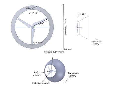
The construction of 3D CAD model of the turbine was performed through the Space Claim module of ANSYS model, and detailed information may be seen in Figure 1.
Figure 1. Geometry specifications and main features of the turbine’s 3D CAD model: A) inlet diameter, B) outlet diameter, C) blade length, D) Blade tip edge distance, E) base length
The rotational velocity (ω) of the turbine’s blades was retrieved from the equation of Tip speed radio (TSR)$=\frac{R^{* \omega}}{V}$, where ω is in rad/s, V is the inlet velocity (m/s) and R the turbine radius (m). The TSR was calculated from the equation for optimal conditions [46]:
$T S R_{\text {optimal }}=\frac{4 * \pi}{n}$ (2)
The calculated TSRoptimal is 4.19, which was adjusted to 3.6 as Hossam et al. recommended [47]. In this sense, the blades rotational velocity (ω) of turbine was 2.51 rad/s.
The Design of Experiments (DOE) considered the ANOVA factorial analysis method to generate statistical information for the further evaluation of the turbine. The design of experiments (DOE) is a planned strategy of measurements and observations integrated by MC, that evaluate independent variables to obtain a response from dependent variables. The factorial ANOVA considers that independent variables affect a dependent variable. The selected factors comprise two or three levels (low, mid and high), which are the minimum, mean and maximum values of the independent variable. The ANOVA uses the results of each MC to determine the main effect and the interaction effects of the factors (independent variables) over the responses (dependent variables). Considering the analyzed design parameters of HT in the literature, this study configured a 23 factorial design with 9 MC, being outlet diameter and blade tip edge distance the factors, and the responses are the shaft pressure, blade tip pressure, pressure over diffuser and downstream velocity the responses; detailed specifications of the design are shown in the results of Table 2.
Table 2. DOE ANOVA factorial design with the operational conditions of the optimization experiment
|
Factors (Independent variables) |
Responses (Dependent variables) |
|||||
|
Modelling case (MC) |
Outlet diameter (m) |
Blade tip edge distance (m) |
Blade tip pressure (Pascal) |
Shaft pressure (Pascal) |
Pressure over diffuser (Pascal) |
Downstream velocity (m/s) |
|
1 |
3.20 |
0.13 |
55,630.60 |
4,665.25 |
487.45 |
1.47 |
|
2 |
3.20 |
0.09 |
35,125.40 |
4,881.59 |
523.08 |
1.51 |
|
3 |
3.20 |
0.04 |
40,703.70 |
5,552.45 |
548.62 |
1.42 |
|
4 |
2.50 |
0.13 |
43,483.40 |
4,806.94 |
302.58 |
1.02 |
|
5 |
2.50 |
0.04 |
38,950.60 |
4,215.52 |
390.53 |
1.14 |
|
6 |
2.50 |
0.09 |
33159.20 |
4356.53 |
329.91 |
1.12 |
|
7 |
2.20 |
0.13 |
36991.80 |
4458.54 |
124.40 |
0.87 |
|
8 |
2.20 |
0.09 |
23922.30 |
5154.08 |
226.84 |
0.77 |
|
9 |
2.20 |
0.04 |
38502.20 |
4137.18 |
226.67 |
0.94 |
The DOE-ANOVA provides the standardized effects of factor over the responses. In this sense, the Eq. (3) is utilized to forecast variables through an ANOVA standardized effect model:
$y=\mu+\frac{\alpha_i}{2} \cdot \hat{X}_i+\frac{\beta_j}{2} \cdot \hat{X}_i+\frac{\delta_{i j}}{2} \cdot \hat{X}_i$ (3)
where, y=dependent variable, μ=Mean of dependent variable, αi=first order effects, βi=second order effects, δi=interactions among effects and $\widehat{X}_i$=normalized factor. The $\hat{X}_i$ is calculated through Eq. (4), where the x is the independent variable (factor) and a, b are the normalized limits -1 and 1 respectively.
$\widehat{X}_i=a+\frac{[x-\min (x)] \cdot(b-a)}{\max (x)-\min (x)}$ (4)
The results of the 9 MC of the DOE-ANOVA (Table 2) showed the minimum and maximum values of the hydrodynamics and mechanics parameters retrieved from the simulation of the turbine through the CFD model. The highest downstream velocity, which could erode the bottom floor of the structure foundation, was 1.51 m/s reported in the MC 2.
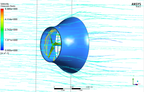
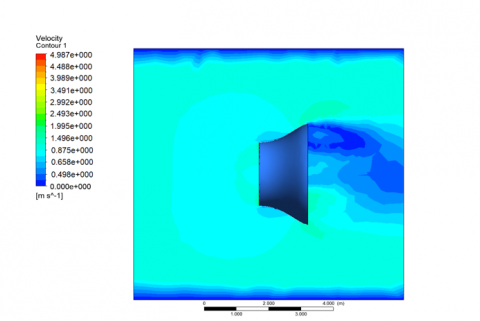
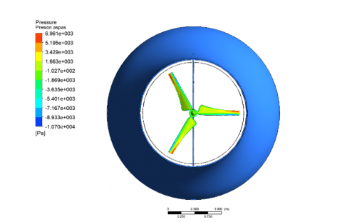
In Figure 2 the numerical results of MC 3 of are shown, pointing the fluid hydrodynamics, rotation field of blades and the maximum hydrodynamic pressure over the structure seen in Table 2. The velocity vectors (Figure 2a) showed magnitudes between 1 m/s (leeward area) to 5.48 m/s (rotational field). The lateral view of the CFD result (Figure 2 b, c) depicted the increment of flow velocity (3.5 m/s) in the lower zone of the downstream area, nearby the exit diameter of the turbine, and a flow velocity of 1.42 m/s close to the bottom (downstream velocity). The maximum Blade tip pressure was reported by the MC 1, however, the MC 3 showed the highest shaft pressure and the pressure over diffuser of 5,552.45 Pa and 548.62 Pa respectively (Figure 2d), which are considered critical for the stability of the turbines support structure. Accordingly, the MC 7 of the DOE-ANOVA (Table 2) may be considered as a proper design for the further optimization, because it reported the lowest pressure and a second lowest downstream velocity.
(a) Velocity vectors
(b) Velocity contour
(c) Flow direction
(d) Blade pressure
Figure 2. CFD results of MC 3 according to the DOE-ANOVA design
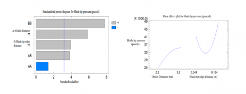
To identify the effects of factors over the responses of all 9 operational conditions, the DOE results were assessed through standardized pareto charts and main effects plot derived from the ANOVA analysis (Figures 3-6). The Blade tip pressure response showed a statistical significance (p-value<0.005), evidencing that outlet diameter (factor) increases the pressure at the tip of the blade (response). The blade tip edge distance factor showed a concave effect over blade tip pressure, then, the inflexion point of concave curve was selected as the most optimal distance from the tip to the edge of the turbine (0.09 m) (Figure 3).
Figure 3. Blade tip pressure experiment analysis
The DOE-ANOVA results seen in the standardized pareto diagram of Shaft pressure showed that vertical blue line did not cut any factor nor combination (A, BB, AA, BB, AB), then, there is not a statistical evidenced (p-value > 0.005) that the factor (Outlet diameter, Blade tip edge distance) affected the Shaft pressure (response). As a result, this response will be omitted for the further optimization process.
Figure 4. Analysis of the Shaft pressure response
The Pressure over diffuser pointed a statistical significance of p-value < 0.005, because vertical blue line cut the factors Outlet diameter (A) and Blade tip edge distance (B), evidencing that these 2 factors influenced the Pressure over diffuser response (Figure 5). The main effect plot noticed that the larger the outlet diameter, the higher the pressure over the diffuser. Also, the increment of blade tip edge distance (factor) reduces the pressure over diffuser (response), then, a 0.134 m value for this factor is considered optimal because the lowest pressure of the response.
Figure 5. Analysis of the pressure over diffuser response
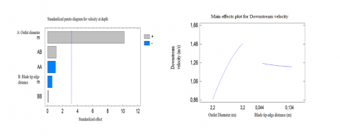
The Figure 6 suggested with statistical significance that the outlet diameter (factor) affects the downstream velocity (response) because the vertical blue line of the standardized pareto diagram only cut this parameter (A). The main effect plots showed a direct effect of the factor, where the bigger is the outlet diameter, the higher is the downstream velocity. Despite of the factor Blade tip edge distance did not show statistical significance, it affected negatively to downstream velocity, what means that the increment of this parameter could reduce the downstream velocity.
Figure 6. Analysis of the downstream velocity response
After the DOE-ANOVA analysis, the results of all MC were selected for calculating parameterized equations to optimize the turbine through the ANOVA standardized effect method. As a result, the Table 3 gathers the estimated effects of the 2 factors (Outlet diameter, Blade tip edge distance) that influenced the 3 main responses (Blade tip pressure, for pressure over diffuser, Downstream velocity).
Table 3. Estimated effects from the DOE ANOVA factorial design
|
Estimated effects for Blade tip pressure (Pa) |
Estimate |
Standard Error |
V.I.F. |
|
Average $(\mu)$ |
32821.2 |
1876.69 |
|
|
A: Outlet diameter |
10384.0 |
1772.27 |
1.05538 |
|
B: Blade tip Edge distance (m) |
7052.7 |
1792.73 |
1.02943 |
|
AA |
-5209.43 |
3746.89 |
1.05333 |
|
AB |
8022.0 |
2108.52 |
1.02737 |
|
BB |
24247.0 |
3111.39 |
1.00412 |
|
Estimated effects for pressure over diffuser (Pa) |
Estimate |
Standard Error |
V.I.F. |
|
Average $(\mu)$ |
429.65 |
20.3508 |
|
|
A: Outlet diameter |
326.37 |
19.2184 |
1.05538 |
|
B: Blade tip Edge distance (m) |
-81.26 |
19.4403 |
1.02943 |
|
AA |
-119.64 |
40.6312 |
1.05333 |
|
AB |
19.01 |
22.8648 |
1.02737 |
|
BB |
-36.22 |
33.7399 |
1.00412 |
|
Estimated effects for Downstream velocity (m/s) |
Estimate |
Standard Error |
V.I.F. |
|
Average $(\mu)$ |
1.23 |
0.0624161 |
|
|
A: Outlet diameter |
0.60 |
0.058943 |
1.05538 |
|
B: Blade tip Edge distance (m) |
-0.04 |
0.0596235 |
1.02943 |
|
AA |
-0.13 |
0.124616 |
1.05333 |
|
AB |
0.08 |
0.0701264 |
1.02737 |
|
BB |
0.01 |
0.10348 |
1.00412 |
Standard errors are based on total error with 3 d.f.
From the DOE-ANOVA results, 3 ANOVA standardized effect models where build using the effects of Table 3:
Blade tip pressure $(P a)=32821.2$$+\frac{10384.0}{2} \cdot \hat{X}_A+\frac{7052.7}{2} \cdot \hat{X}_B$$+\frac{-5209.43}{2} \cdot \widehat{X}_A^2+\frac{8022.0}{2} \cdot \hat{X}_A \hat{X}_B \frac{24247.0}{2} \cdot \hat{X}_B{ }^2$ (5)
pressure over diffuser $(P a)=429.65+\frac{326.37}{2}$$\hat{X}_A+\frac{-81.26}{2} \cdot \widehat{X}_B+\frac{-119.64}{2} \cdot \widehat{X}_A^2+\frac{19.01}{2} \cdot \widehat{X}_A \widehat{X}_B \frac{-36.22}{2}\cdot$$\hat{X}_B^2$ (6)
Downstream velocity $\left(\frac{m}{s}\right)=1.23+\frac{0.60}{2} \cdot \hat{X}_A+$ $\frac{-0.04}{2} \cdot \hat{X}_B+\frac{-0.13}{2} \cdot \hat{X}_A^2+\frac{0.08}{2} \cdot \hat{X}_A \hat{X}_B \frac{0.01}{2} \cdot \hat{X}_B^2$ (7)
The linear regression analysis eased the formulation of 3 models for the HT optimization, where Btp means Blade tip pressure, Pdf is the Pressure over diffuser, Dv is Downstream velocity, Øout means Outlet diameter and Bdis means Blade tip edge distance:
Btp $=6690.67+10127.2 \cdot \emptyset$ out $+56664.3 \cdot$Bdis (8)
$P d f=-393.596+314.357 \cdot \emptyset o u t-916.411\cdot$Bdis (9)
$D v=-0.361672+0.590534 \cdot \emptyset o u t-0.529294 \cdot$Bdis (10)
In this sense, from the CFD results the multiple regression, considering a p-value < 0.005, identified a suitable equation for the turbine optimization. Then, the independent variables of both parameterized equations (ANOVA, Multiple regression) were evaluated using the experimental conditions of the DOE. To identify which equation fit better to the experimental results, the RMSE and the R2 parameters were calculated, where RMSE present the capability of each equation to simulate the CFD results, and the R2 verifies is CFD results is correlated with the results of the Multiple Regression or ANOVA equations, The statistical results of the estimated effects from the DOE ANOVA factorial design are shown (Table 3).
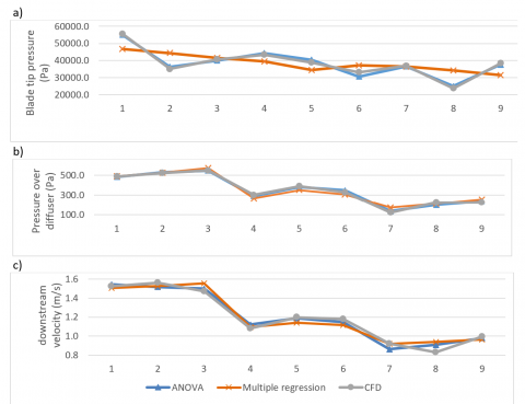
To compare the performance of the ANOVA and Multiple regression methods against the CFD results, the 6 statistical equations E.C (5-10) where evaluated, which consider the experimental conditions of the 9 MC s of the experiment (Table 2). In Figure 7 are shown the results of the 3 main responses modelled through statistical equations and their comparison against the CFD results. The Blade tip pressure results showed a high similarity between ANOVA and CFD models, where the lowest pressure of 23922 Pa occurred in the MC 8. The numerical results of Pressure over diffuser were similar among the three models, being the MC 7 the experimental condition with the lowest pressure 124.41 Pa. The modelled downstream velocity pointed similarity in the numerical results of ANOVA, linear regression and CFD models, being the MC 7 the case with the lowest fluid velocity nearby the bottom. According to the numerical results, the MC 7 is considered an optimal experimental condition because of the lowest pressure over the turbine and the lowest downstream velocity.
The performance of ANOVA and Multiple regression equations (MR) simulating the CFD numerical results was quantitative evaluated thorough linear correlations (R2) and root mean squared errors (RMSE) listed in Table 4. The statistical results of Blade tip pressure showed that R2 validated a high positive linear correlation (0.9756) between ANOVA and CFD, and the limitation of Multiple regression (MR) equations due to their low correlation of 0.3481 when comparing their results against the CFD results. Also, the ANOVA’s RMSE of each MC where significant lower compared to the MR results, where the ANOVA’s MC 9 pointed the lowest value of 289.87 Pa.
Figure 7. Comparison of CFD results against ANOVA and Multiple regression modelled results
The Pressure over diffuser results showed a high correlation (R2 > 0.95) of ANOVA and MR results when compared against the CFD data (Table 4). The ANOVA’s RMSE of this response where lower than MR, being the MC 9 the case with the lowest value (4 Pa).
The statistical results for downstream velocity evidenced that ANOVA and MR simulated properly the CFD data because their R2 > 0.95 and the low RMSE. Hence, the ANOVA equation for downstream velocity E.C (7) outperformed the MR Eq. (10). The low quality of numerical results derived from MR equation in Figure 7(a) could have been due to the restrictions that MR methods face when the order of magnitude increase within the experimental results. However, that assumption could be validated in further experiments testing the capability of MR methods and DOE-ANOVA standardized effect models to simulate the expected results with several ranges and order of magnitude of the response variables.
According to the results mentioned above, the graphs and tables evidenced that ANOVA equations simulated successfully the CFD data. In this sense, was overserved that ANOVA method outperformed the MR method due to the statistical results, where the MR equation of blade tip pressure E.C (8) could not simulate (R2 < 0.3481) the CFD results.
Bouvant et al. [39] performed a DOE-ANOVA to optimize an Archimedes screw turbine using Multiple Regression models (MR) fitting CFD results till finding the best operational conditions. Despite the authors used the advantages of applying ANOVA, they did not formulate optimization equations from the standardized effects, hence they constructed a large second-order regression model with 15 terms, equation that could have been simpler if using ANOVA standardized effect models as we did.
The use of DOE-ANOVA for similar applications is documented in other areas as Oceanography, Ocean Engineering [48-51] and engineering materials [52]. Derschum et al. [53] configured a DOE to examine the effect debris impact over a marine vertical structure under extreme hydrodynamic conditions, and the one-way analysis of variance (ANOVA) determined that there was a significant difference in the mean impact obliqueness between experimental conditions. The studies reviewed in the introduction section about CFD analysis of HT, showed similar hydrodynamic results to this study, which pointed fluid velocities between 0.5 m/s to 2 m/s.
Authors like Fragasso et al. [54] used the DOE-ANOVA method (23 factorial design) to provide a methodology for predicting the reduction of vibration levels generated by a marine Diesel engine and transferred to the ship structure. That study normalized the independent variables and used the standardized effects provided by the DOE-ANOVA to construct a standardized effect model similar to this study. The difference between that study to this research is that Fragasso et al. [54] used experimental data to validate the ANOVA model through a residual analysis, and our study used CFD results to compare the performance of ANOVA standardized effect and Multiple regression models for optimization. In addition, this study goes further than Fragasso et al. [54] study because we analyze the effect of factors over the responses through pareto diagrams and main effect plots, which is fundamental for understanding the non-linear behavior of model design parameters.
According to the DOE-ANOVA results of this study, the outlet diameter of the HT has a positive standardized effect over the design parameters, hence, as the outlet diameters increases, the hydrodynamic pressure over the HT and the downstream velocity rises, Also, the reduction of the blade tip edge distance of HT provokes and increment over the HT responses (Figure 3 to Figure 6). The performance assessment of the ANOVA and Multiple regression models, through their comparison against the CFD results (Figure 7), revealed that ANOVA model outperformed the Multiple regression model during each MC of the experimental conditions set by the DOE (Table 2). In this sense, the DOE-ANOVA method not only provided information about how the factors (Outlet diameter, Blade tip edge distance) affected the responses (Blade tip pressure, Shaft pressure, Pressure over diffuser, Downstream velocity), but also allowed the construction of standardized effect models for future optimization process of the HT.
Table 4. Performance of ANOVA and Multiple regression models for simulating the CFD numerical results
|
|
Blade tip pressure |
Pressure over diffuser |
Downstream velocity |
|||||||||
|
|
ANOVA |
Multiple regression |
ANOVA |
Multiple regression |
ANOVA |
Multiple regression |
||||||
|
MC |
RMSE (Pa) |
R2 |
RMSE (Pa) |
R2 |
RMSE (Pa) |
R2 |
RMSE (Pa) |
R2 |
RMSE (m/s) |
R2 |
RMSE (m/s) |
R2 |
|
1 |
1251.96 |
6470.70 |
13.58 |
28.81 |
0.04 |
0.06 |
||||||
|
2 |
1237.91 |
5743.67 |
13.52 |
28.82 |
0.04 |
0.05 |
||||||
|
3 |
1163.24 |
4835.53 |
13.36 |
28.79 |
0.04 |
0.05 |
||||||
|
4 |
1138.98 |
4826.47 |
13.33 |
27.71 |
0.04 |
0.05 |
||||||
|
5 |
1099.69 |
0.9756 |
4649.80 |
0.3481 |
12.88 |
0.9905 |
25.42 |
0.957 |
0.03 |
0.9732 |
0.05 |
0.9514 |
|
6 |
965.63 |
4407.00 |
12.49 |
21.93 |
0.03 |
0.05 |
||||||
|
7 |
505.44 |
4181.40 |
10.62 |
20.45 |
0.03 |
0.06 |
||||||
|
8 |
493.44 |
4178.96 |
9.54 |
11.48 |
0.03 |
0.06 |
||||||
|
9 |
289.87 |
2346.15 |
4.00 |
10.33 |
0.01 |
0.06 |
||||||
This research configured a Design of Experiment (DOE) - ANOVA combined with Computational Fluid Dynamics (CFD) modelling for the optimization of a HT. The CFD results reported velocities up to 5.48 m/s in the rotational field nearby the rotor blades, and velocities about 3.5 m/s in the lower zone of the downstream area (outlet diameter). The HT Blade tip revealed hydrodynamic pressures in the range of 23,922.30 Pa and 55,630.60 Pa, and the maximum Shaft pressure and Pressure over diffuser were 5,552.45 Pa and 548.62 Pa respectively. The MC 7 of the DOE with an outlet diameter of 2.20 m and Blade tip edge distance of 0.13 m meet the requirements for optimal design of the HT, that considers the lowest hydrodynamic pressures and downstream velocity. In this sense, MC 7 can be selected for the initial shape of the HT model for future optimization processes.
The standardized pareto diagrams evidenced that there was not statistical evidence that Shaft pressure (response) was affected by varying the outlet diameter and blade tip edge distance (factors). As a result, the shaft pressure was not included for the construction of the ANOVA and Multiple regression parameterized equations. Six modelling equations were obtained for the blade tip pressure, pressure over diffuser and downstream velocity dependent variables. The statistical analysis evidenced that ANOVA equations outperformed the Multiple regression equations when simulating the CFD results of the 9 MC of DOE; the Multiple regression equations showed low precision when modelling the MC 1, 2, 4, 5, 6, 8, 9 what provoke a total low R2 of 0.3481.
This research conclude that DOE-ANOVA method is an effective strategy to understanding the effect of varying design parameters over hydraulic and mechanical properties of HT, which provide deterministic equations that may reduce CFD runs in future optimization processes. As future research this work recommends using experimental data for validating the CFD results what will improve the performance of the ANOVA parameterized equations.
[1] Eras, J.J.C., Morejón, M.B., Gutiérrez, A.S., GarcÃa, A.P., Ulloa, M.C., MartÃnez, F.J.R., Rueda-Bayona, F.G. (2019). A look to the electricity generation from non-conventional renewable energy sources in Colombia. International Journal of Energy Economics and Policy, 9(1): 15-25. https://doi.org/10.32479/ijeep.7108
[2] Rueda-Bayona, J.G., Guzmán, A., Eras, J.J.C., Silva-Casarín, R., Bastidas-Arteaga, E., Horrillo-Caraballo, J. (2019). Renewables energies in Colombia and the opportunity for the offshore wind technology. Journal of Cleaner Production, 220: 529-543. https://doi.org/10.1016/j.jclepro.2019.02.174
[3] International Energy Agency (IEA). (2019). World Energy Outlook 2019 – Analysis - IEA, World Energy Outlook 2019. https://www.iea.org/reports/world-energy-outlook-2019.
[4] Salleh, M.B., Kamaruddin, N.M., Mohamed-Kassim, Z. (2019). Savonius hydrokinetic turbines for a sustainable river-based energy extraction: A review of the technology and potential applications in Malaysia. Sustainable Energy Technologies and Assessments, 36: 100554. https://doi.org/10.1016/j.seta.2019.100554
[5] Xu, J., Ni, T., Zheng, B. (2015). Hydropower development trends from a technological paradigm perspective. Energy Conversion and Management, 90: 195-206. https://doi.org/10.1016/j.enconman.2014.11.016
[6] Yuce, M.I., Muratoglu, A. (2015). Hydrokinetic energy conversion systems: A technology status review. Renewable and Sustainable Energy Reviews, 43: 72-82. https://doi.org/10.1016/j.rser.2014.10.037
[7] Behrouzi, F., Nakisa, M., Maimun, A., Ahmed, Y.M. (2016). Renewable energy potential in Malaysia: Hydrokinetic river/marine technology. Renewable and Sustainable Energy Reviews, 62: 1270-1281. https://doi.org/10.1016/j.rser.2016.05.020
[8] Maldar, N.R., Ng, C.Y., Oguz, E. (2020). A review of the optimization studies for Savonius turbine considering hydrokinetic applications. Energy Conversion and Management, 226: 113495. https://doi.org/10.1016/j.enconman.2020.113495
[9] Bersalli, G., Menanteau, P., El-Methni, J. (2020). Renewable energy policy effectiveness: A panel data analysis across Europe and Latin America. Renewable and Sustainable Energy Reviews, 133: 110351. https://doi.org/10.1016/j.rser.2020.110351
[10] Tewari, U., Kolmsee, K., Norta, D. (2015). Hydrokinetic Energy for Enlightening the Future of Rural Communities in Uttarakhand. https://www.semanticscholar.org/paper/Hydrokinetic-Energy-for-Enlightening-the-Future-of-Tewari-Norta/86aba238c132432eeb8f1bd7ee27994486da6805.
[11] Quintero Aguilar, G.E., Rueda Bayona, J.G. (2021). Tidal energy potential in the center zone of the colombian pacific coast. INGE CUC, 17(2). https://doi.org/10.17981/ingecuc.17.2.2021.07
[12] Khan, M.J., Bhuyan, G., Iqbal, M.T., Quaicoe, J.E. (2009). Hydrokinetic energy conversion systems and assessment of horizontal and vertical axis turbines for river and tidal applications: A technology status review. Applied Energy, 86(10): 1823-1835. https://doi.org/10.1016/J.APENERGY.2009.02.017
[13] Nago, V.G., dos Santos, I.F.S., Gbedjinou, M.J., Mensah, J.H.R., Tiago Filho, G.L., Camacho, R.G.R., Barros, R.M. (2022). A literature review on wake dissipation length of hydrokinetic turbines as a guide for turbine array configuration. Ocean Engineering, 259: 111863. https://doi.org/10.1016/J.OCEANENG.2022.111863
[14] Yosry, A.G., Fernández-Jiménez, A., Álvarez-Álvarez, E., Marigorta, E.B. (2021). Design and characterization of a vertical-axis micro tidal turbine for low velocity scenarios. Energy Conversion and Management, 237: 114144. https://doi.org/10.1016/j.enconman.2021.114144
[15] Kirke, B. (2019). Hydrokinetic and ultra-low head turbines in rivers: A reality check. Energy for Sustainable Development, 52: 1-10. https://doi.org/10.1016/j.esd.2019.06.002
[16] dos Santos, I.F.S., Camacho, R.G.R., Tiago Filho, G.L. (2021). Study of the wake characteristics and turbines configuration of a hydrokinetic farm in an Amazonian river using experimental data and CFD tools. Journal of Cleaner Production, 299: 126881. https://doi.org/10.1016/j.jclepro.2021.126881
[17] Alipour, R., Alipour, R., Fardian, F., Koloor, S.S.R., Petrů, M. (2020). Performance improvement of a new proposed Savonius hydrokinetic turbine: A numerical investigation. Energy Reports, 6: 3051-3066. https://doi.org/10.1016/j.egyr.2020.10.072
[18] Shashikumar, C.M., Vijaykumar, H., Vasudeva, M. (2021). Numerical investigation of conventional and tapered Savonius hydrokinetic turbines for low-velocity hydropower application in an irrigation channel. Sustainable Energy Technologies and Assessments, 43: 100871. https://doi.org/10.1016/j.seta.2020.100871
[19] Kirke, B. (2020). Hydrokinetic turbines for moderate sized rivers. Energy for Sustainable Development, 58: 182-195. https://doi.org/10.1016/j.esd.2020.08.003
[20] Chawdhary, S., Angelidis, D., Colby, J., Corren, D., Shen, L., Sotiropoulos, F. (2018). Multiresolution large-Eddy simulation of an array of hydrokinetic turbines in a field-scale River: The Roosevelt Island Tidal Energy Project in New York City. Water Resources Research, 54(12): 10-188. https://doi.org/10.1029/2018WR023345
[21] Verdant_Power. (2020). Verdant Power’s Roosevelt Island Tidal Energy (RITE) Project. https://www.verdantpower.com/projects.
[22] Ocean Renewable Power Company (ORPC). (2012). Tidal Energy Maine Project. https://www.energy.gov/articles/maine-project-takes-historic-step-forward-us-tidal-energy-deployment.
[23] Fernández-Jiménez, A., Cruz, D.F.D.L., Ruiz-Torres, J., Perrino-Blanco, J.L., Jimeno-Almeida, R. (2018). Harnessing the energy of tidal currents: State-of-the-art and proposal of use in EV Charging Points. Multidisciplinary Digital Publishing Institute Proceedings, 2(23): 1504. https://doi.org/10.3390/proceedings2231504
[24] Posa, A., Broglia, R. (2021). Characterization of the turbulent wake of an axial-flow hydrokinetic turbine via large-eddy simulation. Computers & Fluids, 216: 104815. https://doi.org/10.1016/j.compfluid.2020.104815
[25] John, B., Thomas, R.N., Varghese, J. (2020). Integration of hydrokinetic turbine-PV-battery standalone system for tropical climate condition. Renewable Energy, 149: 361-373. https://doi.org/10.1016/j.renene.2019.12.014
[26] Posa, A., Broglia, R. (2021). Momentum recovery downstream of an axial-flow hydrokinetic turbine. Renewable Energy, 170: 1275-1291. https://doi.org/10.1016/j.renene.2021.02.061
[27] Saini, G., Saini, R.P. (2020). Comparative investigations for performance and self-starting characteristics of hybrid and single Darrieus hydrokinetic turbine. Energy Reports, 6: 96-100. https://doi.org/10.1016/j.egyr.2019.11.047
[28] Chimakurthi, S.K., Reuss, S., Tooley, M., Scampoli, S. (2018). ANSYS workbench system coupling: A state-of-the-art computational framework for analyzing multiphysics problems. Engineering with Computers, 34(2): 385-411. https://doi.org/10.1007/S00366-017-0548-4
[29] Ramadan, A., Hemida, M., Abdel-Fadeel, W.A., Aissa, W.A., Mohamed, M.H. (2021). Comprehensive experimental and numerical assessment of a drag turbine for river hydrokinetic energy conversion. Ocean Engineering, 227: 108587. https://doi.org/10.1016/j.oceaneng.2021.108587
[30] Khaled, F., Guillou, S., Méar, Y., Hadri, F. (2021). Impact of the blockage ratio on the transport of sediment in the presence of a hydrokinetic turbine: Numerical modeling of the interaction sediment and turbine. International Journal of Sediment Research, 36(6): 696-710. https://doi.org/10.1016/j.ijsrc.2021.02.003
[31] Lee, J., Kim, Y., Khosronejad, A., Kang, S. (2020). Experimental study of the wake characteristics of an axial flow hydrokinetic turbine at different tip speed ratios. Ocean Engineering, 196: 106777. https://doi.org/10.1016/j.oceaneng.2019.106777
[32] Alizadeh, H., Jahangir, M.H., Ghasempour, R. (2020). CFD-based improvement of Savonius type hydrokinetic turbine using optimized barrier at the low-speed flows. Ocean Engineering, 202: 107178. https://doi.org/10.1016/j.oceaneng.2020.107178
[33] Sarma, N.K., Biswas, A., Misra, R.D. (2014). Experimental and computational evaluation of Savonius hydrokinetic turbine for low velocity condition with comparison to Savonius wind turbine at the same input power. Energy Conversion and Management, 83: 88-98. https://doi.org/10.1016/j.enconman.2014.03.070
[34] Shashikumar, C.M., Madav, V. (2021). Numerical and experimental investigation of modified V-shaped turbine blades for hydrokinetic energy generation. Renewable Energy, 177: 1170-1197. https://doi.org/10.1016/j.renene.2021.05.086
[35] Espina-Valdés, R., Fernández-Jiménez, A., Francos, J.F., Marigorta, E.B., Álvarez-Álvarez, E. (2020). Small cross-flow turbine: Design and testing in high blockage conditions. Energy Conversion and Management, 213: 112863. https://doi.org/10.1016/j.enconman.2020.112863
[36] Tovar, A.M.R., Lopez, Y.U., Laín, S. (2017). Design and prototype of a micro hydrokinetic vertical turbine. Renewable Energy and Power Quality Journal, 1: 903-910. https://doi.org/10.24084/repqj15.512
[37] Muratoglu, A., Tekin, R., Ertuğrul, Ö.F. (2021). Hydrodynamic optimization of high-performance blade sections for stall regulated hydrokinetic turbines using Differential Evolution Algorithm. Ocean Engineering, 220: 108389. https://doi.org/10.1016/j.oceaneng.2020.108389
[38] Labigalini, L.C., de Vasconcelos Salvo, R., de Lima, R.S., da Silva, R.C., de Marchi Neto, I. (2021). Hydrokinetic turbine design through performance prediction and hybrid metaheuristic multi-objective optimization. Energy Conversion and Management, 238: 114169. https://doi.org/10.1016/j.enconman.2021.114169
[39] Bouvant, M., Betancour, J., Velásquez, L., Rubio-Clemente, A., Chica, E. (2021). Design optimization of an Archimedes screw turbine for hydrokinetic applications using the response surface methodology. Renewable Energy, 172: 941-954. https://doi.org/10.1016/j.renene.2021.03.076
[40] Montgomery, D.C. (2019). Design and Analysis of Experiments. Tenth Edit, John Wiley & Sons, Inc., Hoboken, NJ, USA. https://www.wiley.com/en-us/Design+and+Analysis+of+Experiments%2C+10th+Edition-p-9781119492443.
[41] Rueda-Bayona, J.G., Gil, L., Calderón, J.M. (2021). CFD-FEM modeling of a floating foundation under extreme hydrodynamic forces generated by low sea states. Mathematical Modelling of Engineering Problems, 8: 888-896. https://doi.org/10.18280/MMEP.080607
[42] Sarpkaya, T. (1993). Offshore hydrodynamics. Journal of Offshore Mechanics and Artic Engineering, 115: 2-5. https://doi.org/10.1115/1.2920085
[43] Journée, J.M.J., Massie, W.W. (2002). Offshore Hydromechanics. https://ocw.tudelft.nl/wp-content/uploads/OffshoreHydromechanics_Journee_Massie.pdf.
[44] Rueda-Bayona, J.G. (2017). Identificación de la influencia de las variaciones convectivas en la generación de cargas transitorias y su efecto hidromecánico en las estructuras offshore. Universidad Del Norte. http://hdl.handle.net/10584/7629.
[45] Rueda-Bayona, J.G., Horrillo-Caraballo, J., Chaparro, T.R. (2020). Modelling of surface river plume using set-up and input data files of Delft-3D model. Data in Brief, 31: 105899. https://doi.org/10.1016/j.dib.2020.105899
[46] Ragheb, M., Ragheb, A.M. (2011). Wind turbines theory-the betz equation and optimal rotor tip speed ratio. Fundamental and Advanced Topics in Wind Power, 1(1): 19-38. https://doi.org/10.5772/21398
[47] Hossam, S., Aleem, E.A. (2014). Mathematical analysis of the turbine coefficient of performance for tidal stream turbines. https://bura.brunel.ac.uk/bitstream/2438/11044/1/Fulltext.pdf.
[48] Power, H.E., Gharabaghi, B., Bonakdari, H., Robertson, B., Atkinson, A.L., Baldock, T.E. (2019). Prediction of wave runup on beaches using Gene-Expression Programming and empirical relationships. Coastal Engineering, 144: 47-61. https://doi.org/10.1016/j.coastaleng.2018.10.006
[49] Young, D.L., Scully, B.M. (2018). Assessing structure sheltering via statistical analysis of AIS data. Journal of Waterway, Port, Coastal, and Ocean Engineering, 144: 04018002. https://doi.org/10.1061/(ASCE)WW.1943-5460.0000445
[50] Rueda-Bayona, J.G., Guzmán, A., Cabello, J.J. (2020). Selection of JONSWAP spectra parameters for water-depth ans sea-state transitions. Journal of Waterway, Port, Coastal, and Ocean Engineering. https://doi.org/10.1061/(ASCE)WW.1943-5460.0000601
[51] Kotroni, V., Lagouvardos, K., Lykoudis, S. (2014). High-resolution model-based wind atlas for Greece. Renewable and Sustainable Energy Reviews, 30: 479-489. https://doi.org/10.1016/j.rser.2013.10.016
[52] Qasim, A., Nisar, S., Shah, A., Khalid, M.S., Sheikh, M.A. (2015). Optimization of process parameters for machining of AISI-1045 steel using Taguchi design and ANOVA. Simulation Modelling Practice and Theory, 59: 36-51. https://doi.org/10.1016/j.simpat.2015.08.004
[53] Derschum, C., Nistor, I., Stolle, J., Goseberg, N. (2018). Debris impact under extreme hydrodynamic conditions part 1: Hydrodynamics and impact geometry. Coastal Engineering, 141: 24-35. https://doi.org/10.1016/j.coastaleng.2018.08.016
[54] Fragasso, J., Moro, L., Lye, L.M., Quinton, B.W. (2019). Characterization of resilient mounts for marine diesel engines: Prediction of static response via nonlinear analysis and response surface methodology. Ocean Engineering, 171: 14-24. https://doi.org/10.1016/j.oceaneng.2018.10.051