Taha S. Mahmood* | Omar F. Lutfy
© 2022 IIETA. This article is published by IIETA and is licensed under the CC BY 4.0 license (http://creativecommons.org/licenses/by/4.0/).
OPEN ACCESS
This paper presents an intelligent feedforward controller based on the feedback linearization approach to control nonlinear systems. In particular, the nonlinear autoregressive moving average (NARMA-L2) network is trained to reproduce the forward dynamics of the controlled system. Consequently, the trained NARMA-L2 network can be immediately integrated into the inverse feedforward control (IFC) structure. In order to improve the NARMA-L2 structure's ability to approximate nonlinear systems, the NARMA-L2 controller is comprised of two wavelet neural networks (WNNs). In addition, the RASP1 function was used as the mother wavelet function in the structure of the WNN rather than the more common Mexican Hat, Gaussian, and Morlet functions. To prevent the limitations of gradient descent (GD) methods, an artificial gorilla troops optimization (GTO) algorithm is used to determine the optimal settings for the NARMA-L2 inverse controller parameters. In particular, a modified version of the GTO algorithm, which is called the Modified GTO (MGTO) algorithm, is proposed in this work for training the NARMA-L2 inverse controller. This algorithm has demonstrated superior optimization outcomes in comparison to other methods. The effectiveness of the proposed control strategy is demonstrated using two nonlinear dynamical systems. Specifically, several evaluation tests are used to assess the effectiveness of the WNN-based NARMA-L2 in terms of control accuracy and robustness against external disturbances in each of the systems under consideration. These tests clearly demonstrated the effectiveness of the control system. Finally, a comparison study showed that the proposed WNN-based NARMA-L2 controller achieved better control results compared to the multilayer perceptron (MLP) and the radial basis function (RBF)-based NARMA-L2 controllers.
artificial gorilla troops optimization (GTO) algorithm, modified GTO, NARMA-L2, feedback linearization, inverse feedforward controller (IFC), mother wavelet functions
Methods of linear control rely on the presence of a mathematical model of the system. Nevertheless, the majority of physical systems are nonlinear, and their mathematical models are unknown or incompletely understood, and time-dependent. Consequently, conventional techniques are limited in terms of effectiveness and stability [1]. To tackle this difficulty, the artificial neural network (ANN) has been recognized as one of the most effective tools for tracking highly nonlinear dynamic and complex processes due to the rapid advancement of artificial intelligence, which has proven more effective at managing these processes. Neural networks (NNs) can approximate a broad range of nonlinear functions with varying degrees of precision, which makes them useful for identifying and controlling nonlinear dynamic systems [2]. In this regard, the nonlinear autoregressive moving average (NARMA-L2) model is a type of artificial neural network, which was introduced by Narendra and Mukhopadhyay [3]. It is a simple, direct, yet efficient method for reproducing the dynamics of the nonlinear system. The NARMA-L2 model is capable of transforming nonlinear system dynamics into linear dynamics by eliminating the nonlinearities. Consequently, it is best suited for feedback linearization control [4].
There are a number of studies conducted on the NARMA-L2 model. For example, Gundogdu and Celikel [5] proposed an ANN-based NARMA-L2 controller for stepper motor control. They used a backpropagation algorithm (BPA) in order to find the optimal weights for the neural network. Rashad controlled the angular speed of a permanent magnet DC (PMDC) motor's rotor using a NARMA-L2 controller and the dynamic BPA to minimize the mean square of errors [6]. Moreover, El Hamidi et al. [7] proposed a hybrid neural network to establish a multilayer perceptron (MLP) based on NARMA-L2 as a model for controlling a nonlinear MIMO quadcopter system using the BPA to determine the best NN weights. Pedro, and Ekoru [8] used the NARMA-L2 control method for a nonlinear, servo-hydraulic, four-degrees-of-freedom active vehicle suspension. The Levenberg-Marquardt (LM) algorithm was used to train the weights of the network. However, the gradient-based methods, such as the BP and LM algorithms, are distinguished by their slow convergence rates, reliance on a suitable selection of inertial and learning factors, and proclivity to become trapped in local minima of the search space [9].
In designing the IFC structure, an effective inverse model of the system to be controlled must be created. To this end, the neural network is one of the most effective means of addressing IFC design requirements. NNs are well recognized to be universal approximators for a diverse variety of nonlinear functions [10, 11]. In the sequel, the inverse controller based on neural networks has been used a lot to control nonlinear systems. In this respect, most researchers have implemented MLP and RBF NNs within the feedforward control structure. For example, a bearingless induction motor was controlled by MLP NN with 22 hidden layer nodes using an IMC structure [10]. a comparatively large MLP network has been utilized to control unknown nonlinear systems using an IMC scheme [12]. In this method, the IMC structure consisted of two filters: set point and robustness filters. These filters have parameters that can be changed and should be chosen ahead of time, which may make this method less accurate. an arc furnace was controlled using two RBF networks in an IMC structure [13]. The first RBF was used to identify the system, and the system's inverse dynamic was learned using the second RBF. Nonetheless, this control strategy had to go through two stages of training: an identification stage to build a model of the forward plant and a second stage to synthesize the inverse controller.
As another type of neural network, wavelet neural networks (WNNs) are gaining increasing attention from researchers because WNNs combine the theory of wavelets and ANNs to create an integrative method that is more effective. Specifically, WNNs can learn and generalize like ANNs, and they can also navigate like the wavelet transform [14]. Due to these benefits, it has been proven that WNNs are better than other ANNs in terms of their ability to improve the mapping between inputs and outputs [15]. To this end, a comparative study in this paper will show that the WNN is better than both the MLP and the RBF. Despite the above-mentioned attractive features of the WNN, few researchers have implemented the WNN within an inverse controller. For instance, an IMC scheme using a WNN-based NARMA-L2 was used for controlling nonlinear systems [16]. However, this control method necessitates two NARMA-L2 structures, which increases the computational burden. In addition, Alwan [17] utilized a WNN-based NARMA-L2 with the Mexican hat function as the mother wavelet function for the IFC structure. The author utilized the BPA to determine the ideal NN weights.
The performance of the NARMA-L2 controller is directly proportional to the precision of the system's model estimation. The BPA is the most commonly employed learning technique in the literature on NARMA-L2. However, the gradient descent-based BPA has some problems, like a slow rate of convergence and a tendency to get stuck at local minimums in the search space. In order to avoid the limitations mentioned above with gradient-based methods, evolutionary algorithms have gained a lot of attention for their ability to find the global solution to a problem. Therefore, this work focuses on a novel swarm intelligence algorithm known as the Gorilla Troops Optimizer (GTO). Abdollahzadeh et al. [18] originally proposed this algorithm in 2021. GTO was inspired by the way gorillas live as a group and how intelligent they are in social situations. Research so far shows that GTO does a great job on benchmark function optimization [19]. In addition, in order to increase the exploration ability of the original GTO algorithm by adopting more optimal solutions to the optimization process, an enhanced version, termed the modified gorilla troops optimization (MGTO) algorithm, is proposed in this study to optimize the controller's parameters. The simulation results from this study demonstrate that the proposed algorithm is an effective method for optimizing the WNN-based NARMA-L2 network structure.
The principal contributions of this study are summarized in several points. First, a WNN-based NARMA-L2 is proposed to control nonlinear systems using an inverse feedforward controller. The advantage of using a NARMAL2 model is that the proposed method can be used to control unknown nonlinear systems. In particular, only a single NARMA-L2 is needed to learn the controlled plant's forward dynamics, after which the control algorithm can be applied directly without additional training. Second, a modified version of the GTO algorithm called MGTO is proposed for training the WNN to optimize its weights. Finally, utilizing different neural network techniques (MLP and RBF) and the most prevalent activation functions of WNN (Mexican Hat, Gaussian, and Morlet) in the IFC scheme, the proposed control approach demonstrated its superiority via a comparative study. The rest of the paper is organized as follows: Section 2 describes the fundamental principles of the WNN-based NARMA-L2 network. The GTO and its modified version are elaborated upon in Section 3. In Section 4, several performance evaluations and comparative tests are provided to demonstrate the efficacy of the proposed IFC scheme. Finally, Section 5 provides a brief conclusion to the study.
Neural networks are an exceptional mathematical tool for solving nonlinear modeling issues [14]. Consequently, the nonlinear IFC structure is therefore designed by utilizing NNs in this work. In particular, the structure of the NN implemented in this work is known as a nonlinear autoregressive moving average (NARMA-L2) network. It is a powerful neural network architecture for prediction and control [20]. The primary concept behind this approach of control is to use a forward WNN-based NARMA-L2 model of the system to be controlled to create an inverse controller in the IFC structure. In the sections that follow, the WNN's structure and the overall design procedure are discussed.
2.1 WNN structure
Figure 1 illustrates the WNN structure employed in this study. The WNN typically consists of three network layers: an input layer, a hidden (mother wavelet) layer, and an output layer. The function of each layer is outlined below [16, 21]:
Layer 1: This is the input layer, and it is responsible for accepting the input variables (x1, x2, …, xNi) and sending them to the next layer.
Layer 2: This is the hidden layer. It comprises mother wavelet nodes, which are also called "wavelons." In this work, the RASP1 function was utilized instead of the three standard wavelet activation functions (Mexican Hat, Gaussian, and Morlet) [22]. Various experiments with other wavelet functions revealed that the RASP1 function outperforms other functions in the approximation performance [23]. Specifically, this superiority of the RASP1 function in terms of approximation accuracy was proved by a comparative study with other functions, as illustrated in Section 4.5. Moreover, it is worth noticing that the mathematical representation of the RASP1 is relatively simpler than those of the other functions, and this fact is reflected by the shorter processing time taken by the RASP1 compared to the other functions, as shown in Table 3. The following expression represents this function [24]:
$\psi(x)=\frac{x}{\left(1+x^2\right)^2}$ (1)
Consequently, the jth wavelon node's output in this layer can be expressed as:
$\psi_j(x)=\psi\left(z_j\right)$, with $z_j=d_j\left(\sum_{i=1}^{N i}\right.$ $\left.v_{j i} x_i\right)-t_j$ (2)
and
$\psi\left(z_j\right)=\frac{z_j}{\left(1+z_j^2\right)^2}$ (3)
where, tj and dj are the wavelet's translation and dilation factors, respectively, xi is the ith input variable, Ni is the node number of the input layer, and vji is the ith connection weight between the layer of input and the jth wavelon in the mother wavelet layer.
Layer 3: This layer represents output. It is comprised of a single node responsible for calculating the final output of the WNN with the following formula:
$y=\sum_{j=1}^{N w}$ $w_j \psi_j(x)$ (4)
where, Nw represents the number of wavelon layer nodes, and wj denotes the weight of the connection between the jth wavelon node and the output node.
In light of the WNN structure described above, there are several adjustable parameters that must be optimized. The following setting can be used to represent these parameters:
$T=\left[w_j d_j t_j v_{j i}\right]$ (5)
where, Τ represents the adjustable set of parameters. For the WNN structure to function optimally, the parameters in Eq. (5) need to be optimized using an appropriate optimization technique. In this study, these parameters are found using the modified artificial gorilla troops optimizer algorithm, which will be explained in the next sections.
Figure 1. The WNN Structure
2.2 WNN-based NARMA-L2 controller structure
It is necessary to complete two steps in order to make use of the NARMA-L2 control structure considered in this work. These are the stages of system identification and controller design.
2.2.1 Forward plant identification stage
The general structure of the NARMA-L2 model can be expressed by the following formula [20]:
$y(k+1)=f[y(k), y(k-1), \ldots, y(k-n+$1), $u(k-1), \ldots, u(k-n+1)]+g[y(k), y(k-$1), $\ldots, y(k-n+1), u(k-1), \ldots, u(k-n+$1)].u(k) (6)
The NARMA-L2 model necessitates the utilization of two different subnetworks in order to provide an approximation of the functions f and g, as shown in Eq. (6). Both of these subnetworks need (2n-1) input nodes. The two functions $(f$ and $g$ ) in the NARMA-L2 network are approximated using two WNNs in this study.
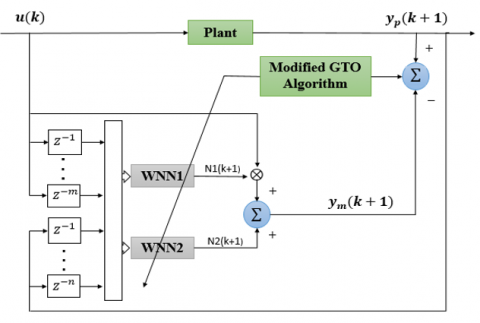
As shown in Figure 2, a series-parallel identification structure performs the NARMA-L2 forward plant identification. In Figure 2, the structure for identification is made up of two WNNs and the input and output tapped delay lines. The modeling error em(k+1) between the output of the actual system yp(k+1) and the NARMA-L2 output ym(k+1) is subsequently utilized to train the NARMA-L2 model. The following equation depicts the NARMA-L2 model output [16]:
$y_m(k+1)=\hat{f}\left(y_p(k), y_p(k-1), \ldots, y_p(k-n+\right.$$1), u(k-1), \ldots, u(k-n+1))+$$\hat{g}\left(y_p(k), y_p(k-1), \ldots, y_p(k-n+1), u(k-1)\right.$$\ldots, u(k-n+1)) \cdot u(k)$ (7)
The process of system identification is carried out utilizing an input-output dataset gathered from the mathematical model of the plant. The MGTO algorithm uses a quadratic cost function as the performance index for training the NARMA-L2 model. The following expression represents this cost function:
$J=\frac{1}{N_P} \sum_{K=1}^{N_P}\left(y_p(k)-y_m(k)\right)^2$ (8)
where, NP represents the number of training patterns, yp(k) represents the output of the plant at time sample k, and ym(k) represents the NARMA-L2 output at time sample k. Throughout the training process, the MGTO algorithm will make the necessary adjustments to the modifiable weights of the WNN-based NARMA-L2 model by minimizing Eq. (8).
2.2.2 Controller design stage
After constructing the NARMA-L2 plant model, the inverse feedforward controller must be formed. This is a straightforward step because the control action could be easily carried out utilizing the identification NARMA-L2 plant model based on Eq. (7). As stated previously, the functions $\hat{f}$ and $\hat{g}$ in Eq. (7) are defined during the stage of the NARMA-L2 plant identification. Furthermore, in order to ensure that the system output yp(k+1) follows the desired reference signal yr(k+1), the following is performed: yp(k+1)=yr(k+1). Consequently, the final output of the NARMA-L2 controller will be as follows [20]:
$u(k)=\frac{y_r(k+1)-\hat{f}\left[y_p(k), y_p(k-1), \ldots, y_p(k-n+1), u(k-1), \ldots, u(k-n+1)\right]}{\hat{g}\left[y_p(k), y_p(k-1), \ldots, y_p(k-n+1), u(k-1), \ldots, u(k-n+1)\right]}$ (9)
Figure 2. WNN-based NARMA-L2 identification model
2.3 The overall structure of the inverse feedforward controller using WNN-based NARMA-L2
The final WNN-based NARMA-L2 IFC structure is shown in Figure 3. It consists of the NARMA-L2 model of the plant identifier based on Eq. (7) and the output of the NARMA-L2 controller based on Eq. (9). The robustness filter in Figure 3 adds robustness to the IFC structure in order to overcome the harmonics of the desired step changes in the set point and to reduce the spikes of the controller's control action. Consequently, the plant's transient period and overshoot are decreased. The robustness filter has the following equation [17]:
$\frac{y_{r e f}(z)}{y_{\text {des }}(z)}=\frac{1-\alpha}{1-\alpha z^{-1}}$
where, α is a tuning parameter.
Figure 3. WNN-based NARMA-L2 IFC structure
Artificial gorilla troops optimization is a newly proposed nature-inspired and gradient-free optimization algorithm that mimics the group lifestyle of gorillas [18]. The gorilla lives in a group known as a troop, which is comprised of an adult male gorilla known as the silverback, multiple adult female gorillas, and their progeny. A silverback gorilla is an adult gorilla named after the distinctive hair on its back during puberty and it lives for more than 12 years. Furthermore, the silverback is the troop's leader. It takes all decisions, mediates conflicts, decides group movements, guides gorillas to sources of food, and ensures the safety of the group. Younger male gorillas aged 8 to 12 years are known as blackbacks because they lack the silvery-colored back hairs of their older counterparts. They are part of the Silverback team and serve as the team's backup defense. Generally, both male and female gorillas prefer to leave the group where they were born and join another one. Conversely, mature male gorillas may separate from the original group and establish their own troops by the attraction of migrating females. Nonetheless, some male gorillas prefer to reside with the original troop and follow the silverback. If the silverback perishes, these males may engage in a violent struggle for group dominance and mate with adult females [19].
3.1 Mathematical model of artificial gorilla troops optimization algorithm
The GTO algorithm's specific mathematical model is developed utilizing the previously mentioned approach of gorilla group behavior in nature. Similar to other intelligent algorithms, GTO is comprised of three major parts: initialization, global exploration, and local exploitation. Each of these is explained in more detail below [19].
3.1.1 Initialization phase
Assume that N gorillas exist in a space of the D-dimension. The i-th gorilla's position in space can be characterized as Xi= (xi,1, xi,2, …, xi, D), i=1, 2, …, N. Accordingly, the gorilla population initialization process can be defined as follows:
$X_{N \times D}=\operatorname{rand}(N, D) \times(u b-l b)+l b$ (11)
where, N represents the population size and D represents the number of variables, and ub and lb are the search space's upper and lower limits, respectively.
3.1.2 Exploration phase
When gorillas leave their original group, they will explore a variety of natural surroundings that they may or may not have encountered previously. All gorillas have assumed candidate solutions in the GTO algorithm, and the silverback is considered to be the best solution in each optimization process. As a way to accurately simulate this kind of natural migration behavior, the gorilla's position update equation for the exploration stage consisted of three distinct methods, which include migrating to unknown locations, migrating around familiar places, and migrating to other groups, as seen in Eq. (12):
$G X(t+1)$$=\left\{\begin{array}{lr}(u b-l b) \times r_2+l b, & r_1<p \\ \left(r_3-c\right) \times X_r(t)+L \times Z \times X(t), & r_1 \geq 0.5 \\ X(t)-L \times\left(\begin{array}{c}L \times\left(X(t)-G X_r(t)\right)+ \\ r_4 \times\left(X(t)+G X_r(t)\right)\end{array}\right) & , r_1<0.5\end{array}\right.$ (12)
where, t denotes the current iteration, GX(t+1) represents the search agents' candidate positions in the next iteration, and X(t) denotes the individual gorilla's current position vector. Moreover, r1, r2, r3, and r4 represent random values between [0, 1], p is a parameter with a range from 0 to 1 that must be set prior to optimization to determine the probability of selecting the migration mechanism to a previously unknown position, Xr(t) and GXr(t) are two locations randomly chosen within the current gorilla population, and Z represents a problem-dimensional row vector with randomly generated values for each element in [-C, C]. Additionally, the parameter C is computed using Eq. (13):
$C=\left(\cos \cos \left(2 \times r_5\right)+1\right) \times\left(1-\frac{I t}{\text { MaxIt }}\right)$ (13)
where, cos denotes the cosine function, r5 denotes a random value between 0 and 1 and it is updated with each iteration, It is the current iteration value, and MaxIt denotes the maximum number of iterations. Finally, the parameter L in Eq. (12) can be calculated as follows:
$L=C \times l$ (14)
where, l represents a random value between -1 and 1.
After the exploration phase is complete, all newly generated candidate solutions GX(t+1) have their fitness values assessed. If GX is superior to X, which is shown by F(GX) < F(X), where F(.) represents the fitness value for a particular problem, it will be kept and will take the place of the original solution X(t). Additionally, silverback Xsilverback is chosen as the best solution for this period.
3.1.3 Exploitation phase
At the time of the troop's formation, the silverback is strong and healthy, whereas the other male gorillas are still juveniles. They abide by all of Silverback's decisions in search of a variety of food resources and satisfy him with unwavering loyalty. Unquestionably, the silverback ages and eventually dies, while younger blackbacks in the troop may engage in violent competition with the other males in the group for mating with adult females and taking over the group. As aforementioned the exploitation phase of GTO models two behaviors: having followed the silverback and competition for adult female gorillas. Simultaneously, the parameter W is established to regulate the switching between them.
If $C \geq W$, the first technique of silverback tracking is selected. The following is the mathematical formula:
$G X(t+1)=L \times M \times\left(X(t)-X_{\text {silverback }}\right)+X(t)$ (15)
where, Xsilverback denotes the best solution found thus far and X(t) represents the gorilla position vector. Additionally, L is calculated using Eq. (14) and the parameter M can be calculated using the formula below:
$M=\left(\mid \frac{1}{N} \sum_{i=1}^N\right.$ $\left.\left.G X_i(t)\right|^{2^L}\right)^{\frac{1}{2^L}}$ (16)
where, N is the size of the population and GXi(t) represents each gorilla's position vector in the current iteration.
If $C<W$, it indicates that the competition for adult female gorillas’ mechanism has been selected and in this case, the gorillas' position can be updated as follows:
$G X(t+1)=$$X_{\text {silverhack }}-\left(X_{\text {silverhack }} \times Q-X(t) \times Q\right) \times A$ (17)
$Q=2 \times r_6-1$ (18)
$A=\varphi \times E$ (19)
$E=\left\{N_1, \quad r_7 \geq 0.5 N_2, \quad r_7<0.5\right.$ (20)
In Eq. (17), X(t) represents the current position and Q represents the impact force, which is calculated by Eq. (18). In addition, the coefficient A utilized to simulate the level of violence in the competition is calculated using Eq. (19), in which φ is a constant value, and the values of E are assigned by Eq. (20), where r6 of Eq. (18) and r7 of Eq. (20) contain random values ranging from 0 to 1. Finally, if r7 > 0.5, E is identified as a 1-by-D array of random numbers with normal distribution, where D is the dimension of space. Otherwise, if r7 < 0.5, E would be equal to a normal distribution-compliant stochastic number.
At the conclusion of the exploitation procedure, the fitness values of the newly created candidate GX(t+1) solution are also computed. If F(GX) < F(X), the solution GX will be maintained and utilized in the next optimization, whereas the best solution among all individuals is denoted by the silverback Xsilverback.
At the conclusion of the exploitation procedure, the fitness values of the newly created candidate GX(t+1) solution are also computed. If F(GX) < F(X), the solution GX will be maintained and utilized in the next optimization, whereas the best solution among all individuals is denoted by the silverback Xsilverback.
3.2 Modified artificial gorilla troops optimization algorithm (MGTO)
Even though the original algorithm attempts to incorporate both exploration and exploitation operations, it has been demonstrated that the GTO tends to get stuck into sub-optimal regions of the search space. This problem is specifically attributable to the original GTO's insufficient exploitation ability. Moreover, equality between exploration and exploitation processes may degrade the algorithm's performance in instances where more exploration operators are required and vice versa [25]. Consequently, training the proposed WNN-based NARMA-L2 in this work resulted in insufficient precision. As a solution to this issue, two modifications have been made in this study to increase the exploration capability of the original algorithm by adopting more optimal solutions to the optimization process. The proposed algorithm was referred to as the Modified artificial gorilla troops optimization algorithm (MGTO). Specifically, as the first modification, the worst n solutions are replaced with new candidate solutions derived from the best solution obtained thus far. In this study, n was set to 20 solutions, and the candidate solutions have been generated using the following formula:
$G X(i, j)=$ Silverback $(j)+\left(G X\left(X_{r 1}, j\right)\right.$$\left.-G X\left(X_{r 2}, j\right)\right) * \mu_{i, j}$ (21)
where, i and j represent the position and dimension of GX, respectively, Silverback is the best solution found so far, Xr1 and Xr2 are two different random integers chosen from 1 to the maximum number of solutions and must be distinct from the index of the current solution, and μi,j represents a random value selected from [-1, 1]. As a second modification, a random solution is generated and its objective function is assessed at each iteration. If this newly generated solution's objective function is worse than the worst solution, the worst solution is replaced with the best solution's position. Instead of that, the worst solution is substituted with the newly generated solution. In order to generate the candidate solution, the following formula was used:
$G X_{\text {worst }}^i= \begin{cases}X_{\text {silverback }}^i & \text { if } J_{\Lambda}^i \geq J_{\text {worst }}^i \\ \Lambda^i & \text { if } J_{\Lambda}^i<J_{\text {worst }}^i\end{cases}$ (22)
where, $\Lambda^i$ represents a random solution value selected from [-1, 1], $J_{\Lambda}^i$ represents the objective function of the random solution and $J_{\text {worst }}^i$ represents the objective function of the worst solution. Notably, these two modifications significantly enhanced the original algorithm's searching capability without the need for additional parameters of control to implement the suggested steps. These characteristics qualify the proposed MGTO to achieve superior optimization results compared to other comparable methods, as illustrated in Section 4.3.
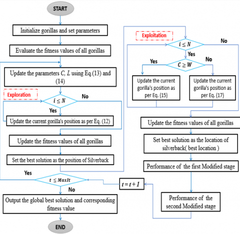
Finally, the steps of the proposed MGTO algorithm are presented in the pseudo-code Algorithm and in Figure 4.
Figure 4. Flowchart of the MGTO
|
Algorithm: Modified Gorilla Troops Optimization |
|
In this section, several tests are conducted to evaluate the WNN-based NARMA-L2 IFC scheme's ability to control complex and nonlinear dynamical systems. In particular, the goal of these evaluation tests is to figure out how well the proposed control method works in terms of how accurate it is and its robustness against external disturbances. To assess how well the proposed MGTO algorithm works at optimizing, a study was done to compare it to other optimization algorithms. In addition, two additional studies were conducted to evaluate the control performance of the WNN-based IFC versus that of other neural network controllers. Particularly, the MLP and RBF, as the principal networks in the IFC. In the second comparison, the RASP1 function will be compared with other wavelet network activation functions. Regarding the MGTO algorithm's control parameters, the population size was set to 50 and the maximum number of iterations was set to 1000. In addition, for every simulation test, the filter tuning parameter $\alpha$ was set to 0.3. These settings for the optimization method's parameters were adequate to ensure the desired control performance.
4.1 Normal performance tests
The objective of these tests is to assess the proposed scheme's control performance with respect to the following nonlinear systems:
Plant 1:
This plant exemplifies the dynamics of a nonlinear system as expressed in the following difference equation [26]:
$\begin{aligned} y(k+1)=& \frac{1.5 y(k) y(k-1)}{1+y^2(k)+y^2(k-1)}+0.1 \times \sin (y(k)+\\ &y(k-1))+1.2 u(k) \end{aligned}$ (23)
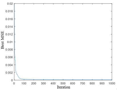
In the IFC scheme, the first design goal is to create a well-trained WNN-based NARMA-L2 forward model of the controlled plant. To accomplish this goal, the training data must cover a significant part of the original system's input-output space. As a result, a random input signal, u(k) (with |u(k)| ≤ 1), was applied to the plant's input defined by Eq. (23), and a training set of 500 input-output data points was made. After that, the WNN-based NARRMA-L2 network's parameters have been optimized using the structure of the series-parallel identification depicted in Figure 2 via the MGTO algorithm in order to reduce the MSE criterion. Figure 6a shows how the MSE decreased over 1000 iterations. After 1000 iterations, the training MSE was 1.075×10⁻⁴. It is important to note that the MGTO algorithm has achieved rapid convergence by minimizing the MSE from the beginning of the optimization process, as shown in Figure 5a. This shows that setting the number of iterations to 1000 seems to be the right choice for the current application.
The performance of the trained WNN-based NARMA-L2 model was evaluated using a separate testing signal in order to assess the precision of the training. The following expression describes this signal for testing [16]:
$u(k)=0.5 \sin \sin \left(\frac{2 \pi k}{25}\right)+0.5 \sin \left(\frac{2 \pi k}{10}\right)$ (24)
Figure 5b depicts the outcome of applying this test signal to the model. The testing signal with an MSE of $2.5206 \times 10^{-4}$ indicates that the WNN-based NARMAL2 model did well in tracking the testing signal. Even though the testing signal was completely different from that used in the training phase, WNN-based NARMA-L2 was able to successfully track it. This indicates that the model has a good ability to generalize.
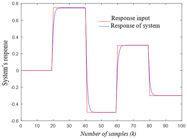
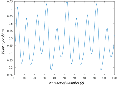
For IFC controller design, it is important to know whether or not the plant model is invertible. This inspection is easy to do by noticing the plant Jacobian sign in the area of interest. In this respect, Figure 5c shows that the plant Jacobian (the coefficient of $u(k)$ in Eq. (9)) is signed definite. This means that the plant model is invertible, which makes it possible to build the inverse controller in the IFC scheme. Figure 5d shows the IFC's excellent control performance in tracking a reference signal, while Figure 5e shows the resulting control signal.
Plant 2:
This plant is a Jacketed Stirred Reactor, also referred to as the Continuously Stirred Tank Reactor (CSTR). The following nonlinear difference formula describes this process's dynamic [27]:
$y(k+1)=0.7653 y(k)-0.231 y(k-1)$$-0.6407 y^2(k)+1.014 y(k-1) y(k)$$-0.3921 y^2(k-1)+0.4801 u(k)$$+0.592 y(k) u(k)-0.5611 y(k-1) u(k)$ (25)
(a) Finest MSE against iterations
(b) The outputs of Plant and the WNN-based NARMA-L2
(c) The Jacobian of the plant
(d) The output response
(e) The control signal
Figure 5. (a-e) Simulation graphs for plant 1
(a) Finest MSE against iterations
(b) The outputs of Plant and the WNN-based NARMA-L2
(c) The Jacobian of the plant
(d) The output response
(e) The control signal
Figure 6. (a-e) Simulation graphs for plant 2
To control the CSTR process, the same control strategy described for Plant 1 was implemented. We began by developing the WNN-based NARMAL2 model using a random input signal u(k). After a few initial iterations, Figure 6a depicts the decrease in MSE as a function of the algorithm's iterations. After 1000 iterations, the training MSE reached 1.055×10⁻⁴. The trained NARMA-L2 model was validated using the same testing signal as in Eq. (25). The resulting modeling performance is demonstrated in Figure 6b, which exhibits excellent modeling of the testing signal with an MSE of 5.390×10⁻⁵. The WNN-based NARMA-L2 performed admirably once again by generalizing its learning to handle the signal of testing that did not exist during the training phase. The plant model is clearly invertible, as shown in Figure 6c. The IFC's control performance is depicted in Figure 6d, with the output signal tracking the reference signal well. Figure 6e depicts the control signal.
4.2 Robustness tests
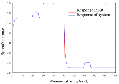
To evaluate the proposed IFC scheme's robustness, a disturbance rejection test has been conducted on each of the plants analyzed in the preceding section. Specifically, five samples of limited disturbances were injected into all of the controlled plants at two different times during the simulation. These periods were 20 ≤ k ≤ 25 and 70 ≤ k ≤ 75. Notably, the IFC scheme had not been learned t to deal with these disturbances, as they were only introduced during the controller testing phase. As shown in Figure 7, the proposed IFC scheme was capable of responding to these unanticipated disturbances by maintaining two plants' responses at the level that was desired.
(a) The output response
(b) The output response
Figure 7. (a and b) Testing of plants 1 and 2 for rejection of disturbance
4.3 A comparative study with other optimization techniques
As stated previously, this paper proposed a modified version of the GTO algorithm called the MGTO algorithm. In this context, a comparison analysis was done with other optimization techniques to show how effective the proposed MGTO is. These techniques include the Genetic Algorithm (GA), the Cuckoo Search Algorithm (CS), and the original GTO. GA and CS are two of the most significant evolutionary algorithm types. The GA has been extensively employed to solve a variety of optimization problems [28] and CS has the potential to be considerably more effective than PSO and GA according to recent studies [29]. In this comparison study, the same plants considered in Section 4.1 were utilized. Because each of the optimization methods under consideration employs multiple random operators, the outcome of a single run of each algorithm may differ from subsequent runs. In order to address this stochastic discrepancy, ten independent runs of each technique for controlling each plant were conducted. The mean of these runs' results has been taken in this study. Table 1 shows the final summary of the results, where Training MSE, Testing MSE, and ISE are the performance measures for the identification and control phases, respectively, and Time is the total processing time, measured in seconds. The MGTO algorithm has achieved the best identification and control outcomes for the two studied plants as demonstrated in Table 1. Specifically, the MGTO algorithm has produced the lowest MSE and ISE values for the two plants when contrasted with the other algorithms. Regarding the processing time, the original version of the GTO was slightly faster than the MGTO. However, in light of MGTO's superior results, this minor discrepancy can be ignored.
Table 1. The performance comparison results of the GA, the CS, the GTO, and the modified GTO algorithms for training the WNN-based NARMA-L2 IFC scheme
|
Optimization methods |
Criterions (average of 10 runs) |
Controlled plants |
|
|
Plant 1 |
Plant 2 |
||
|
GA |
Training MSE |
2.56E-04 |
3.02E-04 |
|
Testing MSE |
40.62E-04 |
40.43E-05 |
|
|
ISE |
3.433 |
3.455 |
|
|
Time (s) |
72.100 |
69.55 |
|
|
CS |
Training MSE |
4.09E-04 |
5.57E-04 |
|
Testing MSE |
50.74E-04 |
70.40E-05 |
|
|
ISE |
3.430 |
3.480 |
|
|
Time (s) |
45.25 |
49.25 |
|
|
GTO |
Training MSE |
1.42E-04 |
1.50E-04 |
|
Testing MSE |
20.23E-04 |
20.62E-05 |
|
|
ISE |
3.424 |
3.457 |
|
|
Time (s) |
41.83 |
46.82 |
|
|
Modified GTO |
Training MSE |
1.09E-04 |
1.20E-04 |
|
Testing MSE |
6.00E-04 |
5.68E-05 |
|
|
ISE |
3.419 |
3.430 |
|
|
Time (s) |
61.88 |
65.96 |
|
4.4 A study comparing other NN-based IFC structure
This section evaluates the performance of the MLP and RBF as the primary networks in the IFC structure in order to compare the WNN's performance with that of other NN types. To ensure a fair comparison, the MLP and RBF networks were trained using the same optimization technique, particularly the MGTO algorithm. In addition, both the MLP and the RBF use the same IFC design process, which was explained in Sections 2.2 and 2.3.
For the MLP, two networks with the same structure were used because the NARMA-L2 necessitates the use of two subnetworks. These networks are made up of three distinct parts: an input layer, a hidden layer, and an output layer. The hyperbolic tangent is used as an activation function by six nodes in the hidden layer, while the linear activation function is used by only one node in the output layer. Similarly, the IFC design under consideration requires two RBF networks. There are three layers in each of these networks: an input layer, a hidden layer, and an output layer. The hidden layer is comprised of six RBF nodes that are distinguished by their centers and widths. As its activation function, the Gaussian kernel function is applied to all nodes in the hidden layer.
Because of the MGTO algorithm's stochastic nature, the outcome of one-run may differ from the outcome of another. As a result, ten separate runs were performed to control each plant using the WNN, MLP, and RBF-based NARMA-L2 IFC structures. Therefore, to figure out how well the three networks perform, we take the average of these ten runs. Table 2 shows a summary of the findings of this study of Plants 1 and 2 that was done in Section 4.1. The results presented in Table 2 demonstrate that the WNN is superior to the MLP and RBF as the primary network in the IFC scheme.
Table 2. The performance comparison results of MLP, RBF, and WNN as the main networks in the IFC structure
|
Type of networks |
Criterions (average of 10 runs) |
Controlled plants |
|
|
Plant 1 |
Plant 2 |
||
|
MLP |
Training MSE |
5.85E-04 |
1.93E-04 |
|
Testing MSE |
50.08E-04 |
20.27E-05 |
|
|
ISE |
3.552 |
4.438 |
|
|
Time (s) |
89.63 |
97.53 |
|
|
RBF |
Training MSE |
20.16E-04 |
50.69E-04 |
|
Testing MSE |
190.61E-04 |
300.88E-05 |
|
|
ISE |
3.977 |
3.595 |
|
|
Time (s) |
68.88 |
67.54 |
|
|
WNN |
Training MSE |
1.09E-04 |
1.20E-04 |
|
Testing MSE |
6.00E-04 |
5.68E-05 |
|
|
ISE |
3.419 |
3.430 |
|
|
Time (s) |
61.88 |
65.96 |
|
4.5 A comparison of the most common WNN activation functions
The primary objective of this study is to evaluate the RASP1 function of the mother wavelet as the activation function, as opposed to the more common Mexican Hat, Gaussian, and Morlet functions. It is well-known that the activation function is one of the most important factors influencing network performance [30]. In terms of those activation functions' structure, they used the same RASP1 function process, which is explained in Section 2.1. Moreover, they were trained using the same optimization method.
As was done before, ten distinct runs were conducted for each of these activation functions to control each plant. To determine the overall performance of these activation functions, we take the average of these ten runs. The results of Plant 1 and Plant 2 are shown in Table 3, which shows that the RASP1 function is better as the mother wavelet in the WNN structure compared to the Mexican Hat, Gaussian, and Morlet functions.
Table 3. The performance comparison results of Mexican Hat, Gaussian, Morlet, and RASP1 as mother wavelet functions in the WW structure
|
Function types |
Criterions (average of 10 runs) |
Controlled plants |
|
|
Plant 1 |
Plant 2 |
||
|
Mexican Hat |
Training MSE |
1.80E-04 |
1.39E-04 |
|
Testing MSE |
20.93E-04 |
20.37E-05 |
|
|
ISE |
3.436 |
3.461 |
|
|
Time (s) |
85.493 |
85.6 |
|
|
Gaussian |
Training MSE |
1.66E-04 |
1.46E-04 |
|
Testing MSE |
40.06E-04 |
20.75E-05 |
|
|
ISE |
3.734 |
3.471 |
|
|
Time (s) |
86.366 |
89.55 |
|
|
Morlet |
Training MSE |
1.88E-04 |
1.42E-04 |
|
Testing MSE |
40.87E-04 |
20.82E-05 |
|
|
ISE |
4.435 |
3.462 |
|
|
Time (s) |
92.82 |
94.35 |
|
|
RASP1 |
Training MSE |
1.09E-04 |
1.20E-04 |
|
Testing MSE |
6.00E-04 |
5.68E-05 |
|
|
ISE |
3.419 |
3.430 |
|
|
Time (s) |
61.88 |
65.96 |
|
This work aims at designing and developing an intelligent control approach based on a WNN-based NARMA-L2 IFC scheme for dynamical nonlinear systems. In this control method, the WNN-based NARMA-L2 network can be trained using a single training phase. The NARMA-L2's structure allows for a direct formulation of the control law, so additional training is not required to find the model inversion. This is a significant advantage of this design method compared to others. The MGTO algorithm, a modified version of the GTO algorithm, was proposed in this study as the training method for determining the optimal settings for the WNN-based NARMA-L2 network's parameters. In comparison to other optimization methods, the MGTO algorithm has given the best results as the optimization technique in the IFC structure. Based on simulation results involving the control of multiple nonlinear systems, the proposed intelligent IFC has demonstrated its efficacy in terms of efficient control performance and robustness against external disturbances. In addition, a comparison study demonstrates that the WNN outperforms the MLP and RBF networks. Finally, in the WNN structure, the RASP1 function is better than the Mexican Hat, Gaussian, and Morlet functions as the mother wavelet function. For future work, the proposed controller will be used in real-time to control a physical system utilizing an adaptive control strategy.
[1] Kumar, R., Srivastava, S., Gupta, J.R.P. (2017). Diagonal recurrent neural network based adaptive control of nonlinear dynamical systems using Lyapunov stability criterion. ISA Transactions, 67: 407-427. https://doi.org/10.1016/j.isatra.2017.01.022
[2] Chen, Y., Zhou, H. (2011). Neural network control approach of a midwater trawl system based on feedback linearization. In Proceedings of 2011 International Conference on Fluid Power and Mechatronics, pp. 138-143.
[3] Narendra, K.S., Mukhopadhyay, S. (1997). Adaptive control using neural networks and approximate models. IEEE Transactions on Neural Networks, 8(3): 475-485. https://doi.org/10.1109/72.572089
[4] Jibril, M., Tadesse, M., Hassen, N. (2021). Temperature control of a steam condenser using NARMA-L2 Controller. Journal of Engineering and Applied Sciences, 16(10).
[5] Gundogdu, A., Celikel, R. (2021). NARMA-L2 controller for stepper motor used in single link manipulator with low-speed-resonance damping. Engineering Science and Technology, an International Journal, 24(2): 360-371. https://doi.org/10.1016/j.jestch.2020.09.008
[6] Rashad, L.J. (2010). Speed control of permanent magnet DC motor using neural network control. Eng. & Tech Journal, 28(19): 5844-5856.
[7] El Hamidi, K., Mjahed, M., El Kari, A., Ayad, H., El Gmili, N. (2021). Design of hybrid neural controller for nonlinear MIMO system based on NARMA-L2 model. IETE Journal of Research, pp. 1-14. https://doi.org/10.1080/03772063.2021.1909507
[8] Pedro, J., Ekoru, J. (2013). NARMA-L2 control of a nonlinear half-car servo-hydraulic vehicle suspension system. Acta Polytechnica Hungarica, 10(4): 5-26.
[9] Huang, H.X., Li, J.C., Xiao, C.L. (2015). A proposed iteration optimization approach integrating backpropagation neural network with genetic algorithm. Expert Systems with Applications, 42(1): 146-155. https://doi.org/10.1016/j.eswa.2014.07.039
[10] Wang, Z.Q., Liu, X.X. (2013). Nonlinear internal model control for bearingless induction motor based on neural network inversion. Acta Automatica Sinica, 39(4): 433-439. https://doi.org/10.1016/S1874-1029(13)60043-9
[11] Zhao, Z.C., Liu, Z.Y., Xia, Z.M., Zhang, J.G. (2012). Internal model control based on LS-SVM for a class of nonlinear processes. Physics Procedia, 25: 1900-1908. https://doi.org/10.1016/j.phpro.2012.03.328
[12] Li, H.X., Deng, H. (2006). An approximate internal model-based neural control for unknown nonlinear discrete processes. IEEE Transactions on Neural Networks, 17(3): 659-670. https://doi.org/10.1109/TNN.2006.873277
[13] Yu, F., Mao, Z. (2012). Internal model control for electrode in electric arc furnace based on RBF neural networks. In 2012 24th Chinese Control and Decision Conference (CCDC), pp. 4074-4077. https://doi.org/10.1109/CCDC.2012.6244650
[14] Lutfy, O.F. (2014). Wavelet neural network model reference adaptive control trained by a modified artificial immune algorithm to control nonlinear systems. Arabian Journal for Science and Engineering, 39(6): 4737-4751. https://doi.org/10.1007/s13369-014-1088-5
[15] Chen, C.H. (2011). Intelligent transportation control system design using wavelet neural network and PID-type learning algorithms. Expert Systems with Applications, 38(6): 6926-6939. https://doi.org/10.1016/j.eswa.2010.12.031
[16] Lutfy, O.F., Selamat, H. (2015). Wavelet neural network-based narma-l2 internal model control utilizing micro-artificial immune techniques to control nonlinear systems. Arabian Journal for Science and Engineering, 40(9): 2813-2828. https://doi.org/10.1007/s13369-015-1716-8
[17] Alwan, Y.H. (2012). A proposed wavenet identifier and controller system. Book, LAP LAMBERT Academic Publishing.
[18] Abdollahzadeh, B., Soleimanian Gharehchopogh, F., Mirjalili, S. (2021). Artificial gorilla troops optimizer: A new nature‐inspired metaheuristic algorithm for global optimization problems. International Journal of Intelligent Systems, 36(10): 5887-5958. https://doi.org/10.1002/int.22535
[19] Xiao, Y., Sun, X., Guo, Y., Li, S., Zhang, Y., Wang, Y. (2022). An improved gorilla troops optimizer based on lens opposition-based learning and adaptive β-hill climbing for global optimization. CMES - Computer Modeling in Engineering and Sciences, 130(3). https://doi.org/10.32604/cmes.2022.019198
[20] Kassem, A.M. (2012). MPPT control design and performance improvements of a PV generator powered DC motor-pump system based on artificial neural networks. International Journal of Electrical Power & Energy Systems, 43(1): 90-98. https://doi.org/10.1016/j.ijepes.2012.04.047
[21] Farahani, M. (2013). Intelligent control of SVC using wavelet neural network to enhance transient stability. Engineering Applications of Artificial Intelligence, 26(1): 273-280. https://doi.org/10.1016/j.engappai.2012.05.006
[22] Khan, M.M., Mendes, A., Chalup, S.K. (2020). Performance of evolutionary wavelet neural networks in acrobot control tasks. Neural Computing and Applications, 32(12): 8493-8505. https://doi.org/10.1007/s00521-019-04347-x
[23] Lutfy, O.F. (2020). An integrated feedforward-feedback control structure utilizing a simplified global gravitational search algorithm to control nonlinear systems. Sādhanā, 45(1): 1-16. https://doi.org/10.1007/s12046-020-01491-2
[24] Almallah, A.S., Zayer, W.H., Alkaam, N.O. (2014). Iris Identification Using Two Activation Function Wavelet Networks. ALMALLAH et al., Orient. J. Comp. Sci. & Technol, 7: 265-271.
[25] Abdel-Basset, M., Mohamed, R., Chang, V. (2021). An efficient parameter estimation algorithm for proton exchange membrane fuel cells. Energies, 14(21): 7115. https://doi.org/10.3390/en14217115
[26] Lutfy, O.F., Majeed, R.A. (2018). Internal model control using a self-recurrent wavelet neural network trained by an artificial immune technique for nonlinear systems. Engineering and Technology Journal, 36(7 Part A): 784-791. https://doi.org/10.30684/etj.36.7a.11
[27] Pearson, R.K., Kotta, Ü. (2004). Nonlinear discrete-time models: state-space vs. I/O representations. Journal of Process Control, 14(5): 533-538. https://doi.org/10.1016/j.jprocont.2003.09.007
[28] Anwer, A., Almosawi, A.H. (2022). A dynamic optimal power flow of a power system based on genetic algorithm. Engineering and Technology Journal, 40(2): 290-300. http://doi.org/10.30684/etj.v40i2.1747
[29] Gandomi, A.H., Yang, X.S., Alavi, A.H. (2013). Cuckoo search algorithm: a metaheuristic approach to solve structural optimization problems. Engineering with Computers, 29(1): 17-35. http://doi.org/10.1007/s00366-012-0308-4
[30] Feng, J., Lu, S. (2019). Performance analysis of various activation functions in artificial neural networks. In Journal of Physics: Conference Series, 1237(2): 022030. http://doi.org/10.1088/1742-6596/1237/2/022030