Juan G. Rueda-Bayona* | Andrés Guzmán | Andrés F. Osorio
© 2022 IIETA. This article is published by IIETA and is licensed under the CC BY 4.0 license (http://creativecommons.org/licenses/by/4.0/).
OPEN ACCESS
Sea extreme events affect the integrity and operation of the offshore structures, then, it is important to analyze wind-waves-currents loads over the structural dynamics. Traditional offshore designing identifies structural parameters with certain limitations: physical modeling involves using shaking tables in dry conditions; numerical simulations have not sufficiently considered the effects of combined extreme waves-wind-current loads over the structure and the significance of the near and far hydrodynamic field over the structure. The non-linear interactions in the near hydrodynamic field generate viscous damping that modifies the dynamic structural parameters of the offshore structures. The traditional determination of structural parameters considers the hydrodynamic forces computed from wave records, omitting fluid-structure interactions that could generate unexpected damped periods and amplification peaks. This study applied physical modeling to determine floating structural parameters, considering combined loads and the effect of far and near hydrodynamic field in the fluid-structure interaction. The calculated transfer functions in the near hydrodynamic field revealed the highest amplification of the structural accelerations, and the transfer functions in the far field did not evidence structural resonance. Finally, this study recommends measuring the near hydrodynamic field and applying DOE-ANOVA for offshore designing to assess the viscous damping that may provoke dangerous structural amplifications.
structural dynamics, floating foundation, Duhamel method, half-power bandwidth method, DOE, ANOVA
The interest in developing new renewable energy projects is worldwide, with important investments for research and technology [1, 2]. The marine and offshore energy projects face extreme sea-states generated by Hurricanes, Typhoons, Cold-fronts, and other oceanographic events affect their functioning and put on risk the structural integrity [3-5]. When an extreme sea-state occurs at an offshore wind field, the security systems interrupt the energy production stopping the blades rotary motion (pitch control or blade feathering) [6].
The need to develop effective damping systems for offshore structures that face normal and extreme sea-states [7] motivated the utilization of numerical and physical modeling to analyze structural parameters [8-13]. Kandasamy et al. [14] mentioned that environmental loads (wind, waves, and currents) had affected the operability of the offshore structures generating accidents aboard and structural failures during the last decades.
Ou et al. [15] developed a damping isolation system to control vibrations of a jacket platform. Mojtahedi et al. [16] applied forced vibration tests to analyze the structural health during several damage conditions. Hosseinlou and Mojtahedi [17] analyzed a physical scaled model of a jacket offshore structure through vibration tests in dry conditions (without considering the effect of water) to identify the initial parameters for numerical modeling suitable to analyze the structural health. Other studies built physical models of offshore structures and did not analyze the near hydrodynamic field of the structure during unperturbed and perturbed conditions [9, 16, 17].
Several studies analyzed the structural responses of fixed and floating structures because of the linear and non-linear wind, waves and currents loads, which estimated the natural and damped period of these structures [18-27]. Shirzadeh et al. [28] recommended experimental studies to analyze the structural behavior of offshore structures during wind and wave loads, including wind damping contribution. Also, Subbulakshmi and Sundaravadivelu [29] pointed out the hydrodynamic vortex importance on the structural damping. Several other studies applied wave loads calculated from a synthetic-free surface record using the JONSWAP spectra to excite the structure under analysis. Wei et al. [30] estimated damping considering the effect of wave heights over the structural deformation but not considered the effect of wave periods. Skaare et al. [27] assessed the response of a floating wind turbine model through the computer programs SIMO/RIFLEX and HAWC2, and validated the simulations with experimental results preformed at a wave basin (50 m * 80 m); the study did not consider the ocean current loads during extreme sea states. These studies did not show details of the fluid-structure interaction because of the currents and generated vortex during the wave approximation into the structure [19, 24, 30-33].
The most applied equations to determine structural damping and natural periods are the logarithmic decrement method and the Half-Power Bandwidth Method [34, 35]. Carswell et al. [36] used the logarithmic decrement method to determine the critical damping of an offshore wind turbine foundation. Koukoura et al. [37] identified the structural damping of two oscillation modes of a monopile offshore wind turbine. Also, they applied the discrete Fourier transform to analyze spectral curves through the Half-Power Bandwidth Method. Their study recommended filtering spurious records by eliminating harmonics in the time series to identify a proper structural damping. Van Der Tempel et al. [38] recommended the Half-Power Bandwidth Method for determining the structural parameters in the design of support structures for offshore wind turbines. In addition, the study suggests applying the logarithmic decrement method to select the periods and damping of each experimental condition. Then, the author did a linear regression to select statistically representative values for structural periods and damping.
The numerical modeling is considered an alternative to evaluate non-linear responses of the offshore structures because of wind, waves and current loads [30, 31, 39, 40]. Colwell and Basu [32] applied the Kaimal and Jonswap spectra to generate wind and wave loads to analyze the structural response of an offshore wind turbine. Shi et al. [33] used the JONSWAP spectra to generate wave loads and performed a modal analysis of an offshore wind turbine considering the wind and waves states of the Korean southeast sea.
Despite the numerical modeling may be a flexible and economical alternative to determine structural dynamic parameters, some non-linearities that affect the structural dynamics might be ignored. The physical modeling with instrumented scaled models in tanks or wave channels is a complementary approach for offshore designing, which could reveal complex fluid-structure interactions not reported by the numerical simulations. Also, the determined damping characteristics of the scaled models must be carefully transferred to the full-scale design according to recommended scaling rules and maximum model scale (1:100) [41-43].
Most of the above-reviewed literature analyzed fluid-structure interactions with transfer functions using wave loads numerically generated by 1D equations such as Pearson-Moskovitz and JONSWAP spectra. Also, those studies applied forced vibration methods with independent loads and physical models in dry conditions (without the presence of water) what could omit non-linear interactions of wind, waves and currents that affect the structural dynamic parameters [44]. The literature review revealed the lack of information on the physical modeling of fluid-structure under extreme sea-state conditions for floating structures and when blades rotation is restricted due to high wind loads.
According to the aforementioned findings and lack of information, the present study proposes an alternative approach to determine structural dynamic parameters in damped (water) conditions through the excitation of a floating structure with combined loads (wind, waves and currents). The viscous effect of water over the structural damping parameters was assessed through the Half-Power Bandwidth Method, Duhamel integral, and the Logarithmic Decrement method. Finally, this study performed a DOE-ANOVA (Design of Experiments- Analysis of Variance) analysis of the effect of water level records and 3D velocity measurements over the structure accelerations to identify the influence of wave loads (far field) and the current loads in the near field over the structural dynamics.
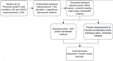
This study proposes a different approach to estimate the structural parameters (periods and damping ratios) of offshore structures as follows (Figure 1):
Figure 1. Proposed methodology for calculating structural parameters of offshore structures
(1) Model set up: configure the physical model in a wet condition provided by a tank or wave channel. Install free surface and velocity measurement instruments. Perform the DOE [45] to take into account several experimental conditions for the wind, waves and currents loads.
(2) Undisturbed-damped natural periods: apply impulsive loads (e.g., the pulling method described in Section 2.2 Model set up), then measure the load and structural responses for undisturbed wet conditions (without loads) to determine the damped natural periods using the Logarithmic Decrement method.
(3) Disturbed-damped natural periods: apply wind, waves, and currents loading as per the DOE and measure the loads and structural responses to estimate disturbed-damped natural periods using the Half-Power Bandwidth Method [34].
(4) Damping ratios: Utilize the frequencies of the Half-Power Bandwidth Method for determining the damping ratios (ζ=zeta). In addition, build pseudo-displacement and pseudo-acceleration graphs through Duhamel integral [34] to determine additional damping ratios (ξ=xi).
(5) Fluid-structure interaction: Using Pareto charts and standardized effects graphs from ANOVA analysis [45], identify the effect of factors (loads) over the structural responses and set recommendations for the structural damping.
2.1 Model set up
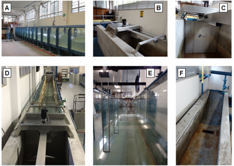
In order to control the experimental conditions of the DOE, was required the utilization of a wave flume (Figure 2), with 25.0 m long, 1.0 m wide, and 1.0 m of height. The generation area is 4.0 m long with a bi-directional pump for the current generation (1.5 m/s of maximum velocity), followed by the propagation zone (15.0 m) (Figure 2a). Next appears the dissipation zone with 6.0 m of length. A 3D Acoustic Doppler Velocimeter (ADV; Sontek 3DVS) (Figure 2b) was located to 0.08 m upstream from the wind turbine (Figure 2c) to measure the near hydrodynamic field and worked at 80 Hz with a vertical recording profile of 0.07 m from the bottom. Considering the recommendations of Chakrabarti [46], was placed a pulling system with a dynamometer to simulate wind loads nearby to the structure. Because of each run of the experiment lasted 30 seconds approximately, the pulley system is considered proper because this elapsed time may be related to a wind gust; further details will be given next (Figure 2d). Four wave gauges (Figure 2e) were positioned every 1.76 m (characteristic wavelength) from the centroid of the wind turbine (physical model with 1:50 scale) and recorded to a frequency of 100 Hz. At the end of the channel is placed a beach integrated by gravel material (Figure 2f) to dissipate waves and reduce internal reflections. The water level at the wave flume was set to 0.40 m (distance between the bottom and the free surface). A general view of the wave flume with its main sections such as generation, propagation and dissipations zones are shown in Figure 2.
Figure 2. Wave channel arrangement and instrument localization: a) wave paddle, b) 3D velocity current sensor (3DVS), c) wind turbine, d) pulling system with a dynamometer, e) 4 water level sensors (resistive), f) beach with gravel material. Axes units in meters
The design of the physical model (Figure 3) aims to understand the effect of water viscous damping over the dynamic parameters under extreme excitation of a scaled floating structure; then, its geometry may be considered as coarse and general for commercial designing but meaningful for the understanding of the fluid-structure interaction of this study. The scaled (1:50) dimensions of the physical model (0.36 kg of total weight) stabilized with four (4) mooring lines (nylon) are described as follows:
The wind turbine was monitored with a pre-installed tri-axial accelerometer with a measuring rate of 200 Hz (Figure 3f). Wind loading was applied through a constant pulling method where cables pull the blades; a dynamometer was used to measure the applied tractions (Figure 3g). The pulling method is applicable when the experiment considers that blades face strong wind-gust or extreme events such as hurricanes. In that situation, the pitch control stops the rotation of the blades and turns the blades to be parallel to the airflow (feathering over blades). As a result, the pulling method represents the extreme wind loads over stopped blades The wind loads are associated to typical extreme values derived from hurricanes [47], then, 50 g = 54.85 m/s (197.45 km/h) correspond to a hurricane category 3, 150 g=95 m/s (342 km/h) to a hurricane category 5, and a maximum of 250 g=122.65 m/s (441.54 km/h)>hurricane category 5.
Figure 3. Physical model (1:50) of the offshore wind turbine: a) water level sensor, b) 3D velocity sensor (3DVS), c) wind turbine, d) mooring lines, e) pulling system with a dynamometer, f) accelerometers, g) wind load mechanism
2.2 DOE-ANOVA
The DOE is a methodology for gathering information through measurements and observations of the response of dependent variables (structural accelerations) under the effect of independent variables (waves, wind, and currents loads) known as factors. The DOE considers the mean, minimum and maximum values of the known factors to set two or three levels (low, middle, and high). The collected information is verified by fulfilling three assumptions (normality, independence and homoscedasticity) before applying the ANOVA analysis.
The ANOVA reveals the main effect and non-linear interactions of the factors over the responses, considering the behavior of variance among the analyzed variables. The DOE-ANOVA assigns identifiers and values for each factors’ level. For example, wave loads may have three levels: low (A-), middle (A) and high (A+). When a factor interacts with other, waves (A) and wind (B) loads, they may be denoted as AB. With the aforementioned notation of factors, graphs such as Pareto charts and primary effect plots evidence the effects of factors over the responses. The Pareto charts utilize bars that represent the absolute values of the standardized effects, and a vertical line reveals which effects are statistically significant. On the other hand, the main effect plots warn if the factors and responses are linear or non-linearly related.
The DOE-ANOVA have been applied in several studies related to offshore engineering [48], coastal engineering [49, 50], and in a previous study of wave hydrodynamics performed by the authors [51].
The Design of Experiment (DOE) of this study was configurated for three experimental conditions. For the first condition (Condition 1), the wave paddle generated irregular waves by means of the JONSWAP spectra to excite the floating structure. In the second condition, the structural excitation generated by the irregular waves is complemented with a constant wind loading (Condition 2). For the third experimental condition, waves, wind, and currents loads were applied simultaneously (Condition 3); the JONSWAP spectra was performed with gamma = 1. Table 1 shows the 27 runs of the experiment.
Table 1. Design of Experiment (DOE) with three experimental conditions; g represents mass units
|
Condition 1 |
Condition 2 |
Condition 3 |
|||||
|
Run |
Hs (m) |
Tp (s) |
Run |
Wind load (g) |
Run |
Currents velocity (cm/s) |
Wind load (g) |
|
1 |
0.09 |
1.76 |
10 |
50 |
19 |
10 |
50 |
|
2 |
0.09 |
1.49 |
11 |
50 |
20 |
10 |
50 |
|
3 |
0.09 |
1.20 |
12 |
50 |
21 |
10 |
50 |
|
4 |
0.07 |
1.76 |
13 |
150 |
22 |
10 |
150 |
|
5 |
0.07 |
1.49 |
14 |
150 |
23 |
10 |
150 |
|
6 |
0.07 |
1.20 |
15 |
150 |
24 |
10 |
150 |
|
7 |
0.05 |
1.76 |
16 |
250 |
25 |
10 |
250 |
|
8 |
0.05 |
1.49 |
17 |
250 |
26 |
10 |
250 |
|
9 |
0.05 |
1.20 |
18 |
250 |
27 |
10 |
250 |
Note: Hs and Tp are the same for Condition 2 and Condition 3, from top to bottom, accordingly to the Condition 1.
The Hs and Tp values are associated with extreme sea-states and were numerically scaled considering the linear wave theory. Reported ocean current and wind velocities during extreme events were taken from the literature [52, 53]. A value of 10 cm/s was set for the experiment in order to avoid hydrodynamic reflection by the channel’s walls and for protecting the integrity of the floating structure.
3.1 Undisturbed-damped natural periods
We performed five (5) free vibration tests for 3 degrees of freedom (x, y, z) to determine the undisturbed-damped natural period in water. The procedure included pulling the hub of the wind turbine through cables and then releasing the turbine to get free vibrations. Then, we measured the x longitudinal acceleration (surge), y transversal acceleration (sway) and the z vertical acceleration (heave), as shown in Figure 4.
The acceleration records for the three degrees of freedom derived from the five undisturbed free vibration tests (Figure 4), were used to determine the damped natural periods (Tn) and damping ratios (z, zeta) through the Logarithmic Decrement method. The five (5) undisturbed free vibration tests allowed identifying the mean damped natural periods for the wet undisturbed conditions: 1.12 s for surge, 0.7 s for sway and 0.52 s for heave (Table 2).
The damping ratios represent the ratio between the damping coefficient and the critical damped coefficient [34] where:
$\zeta, \xi$ =1 denotes a critically damped system.
$\zeta, \xi$ >1 denotes an over damped system.
$\zeta, \xi$ <1 denotes an underdamped system.
Figure 4. Undisturbed free vibration tests in wet conditions
Table 2. Mean damped natural periods and damping ratios derived from the application of the Logarithmic Decrement method
|
Tn (s) |
($\zeta$, zeta) |
($\zeta$, zeta) % |
|
|
surge |
1.12 |
0.00047512 |
0.047 |
|
sway |
0.70 |
0.06167408 |
6.167 |
|
heave |
0.52 |
0.00080432 |
0.080 |
3.2 Disturbed-damped natural periods
A Fourier analysis was performed to every acceleration record (loads and responses) derived from the runs (Table 1) to determine the damped natural periods during water perturbed conditions. The acceleration spectra generated by Fourier allowed selecting the associated period of significant acceleration required by the transfer functions of the Half-power Bandwidth Method. In Figure 5, Figure 6 and Figure 7 are plotted the transfer functions where the x-axis corresponds to the excitation frequency (load) and the y-axis corresponds to the normalized acceleration (structural acceleration / load acceleration). In order to analyze the difference in calculating the transfer functions with water level records measured in the far field and velocity records of the near field, the plot results were labeled SN and 3DVS, respectively. The SN identifier represents the transfer plots calculated with the water level records (far field) measured by the closest water level sensor located upstream to the structure, and the 3DVS identifier represents the transfer plots calculated with the 3D velocity records in the near field (Figure 1). The aforementioned transfer function plots do not have an equal excitation frequency scale in order to ease the identification of the amplification peaks and for keeping proportional the visualization of the curves because of small sizings of some graphs.
The transfer function of the longitudinal movements in x (surge) pointed that runs with no currents loads showed two amplification peaks, possibly by the induced damping because of the mooring lines (Figure 5a, b, d, e). Also, the Condition 2 registered by the 3DVS (Figure 5e) showed a concentrated amplification effect compared to the distributed amplification in the transfer function derived from the SN records (Figure 5b). The runs with current loads (Figure 5c, f) did not show two peaks compared to the other transfer functions (Figure 5a, b, d, e), showed a uniform distribution instead. The transfer function derived from 3DVS (Figure 5f) had a higher amplification peak compared to the amplification of the transfer function of the SN (Figure 5c).
Figure 5. Damped natural periods in the x displacements (Surge) through the Half Bandwidth Method (Transfer function plots)
The transfer functions of the sway movements pointed out that Condition 1 runs showed two amplification peaks (Figure 6 a,d), similar to the evidenced in the surge conditions (Figure 5). We also noticed that Condition 2 (Figure 6e) had a lesser effect in the structural amplification (normalized acceleration increment) compared to the Condition 2 calculated with the SN (Figure 6b).
Figure 6. Damped natural periods in the y displacements (Sway) through the Half Bandwidth Method (Transfer function plots)
The transfer functions derived from the Condition 3 (Figure 6c,f) showed a more distributed curve, similar that occurred in the runs with surge displacements (Figure 5c,f). In addition, the transfer function of 3DVS runs in sway conditions (Figure 6f) showed a higher amplification compared to the SN transfer function (Figure 6c), similar to what occurred in the transfer functions in surge conditions (Figure 5c,f).
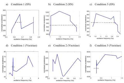
The transfer functions derived from z displacements (heave, Figure 7) showed a similar behavior compared to the surge and sway movements (Figure 5, Figure 6). Condition 1 and Condition 2 showed the highest amplification in the SN records (Figure 7). During Condition 3, the 3DVS records generated a distributed transfer function curve with a higher amplification compared to the curves derived from the SN records. Table 3 gathers the natural damped periods of the floating structure during disturbed conditions; the fail notation denotes that the transfer function curve had not the shape to perform properly the Half Bandwidth Method. The identifiers ω1, ω2 are the selected angular frequencies from the peak frequency (ωp) in order to determine the natural damped period (TD) through the Half Bandwidth Method.
Figure 7. Damped natural periods in the z displacements (Heave) through the Half Bandwidth Method (Transfer function plots)
Table 3. Natural damped periods (TD) for the 3 degrees of freedom of the floating structure during disturbed conditions
|
Surge – x |
$\omega_{1}$ (Hz) |
$\omega_{2}$ (Hz) |
$\omega_{p}$ (Hz) |
zeta |
TD (s) |
|
Condition 1 (3DVS) |
2.00 |
2.75 |
2.56 |
0.16 |
0.39 |
|
Condition 1 (SN) |
0.63 |
0.69 |
0.66 |
0.04 |
1.52 |
|
Condition 2 (3DVS) |
0.26 |
0.29 |
0.27 |
0.05 |
3.76 |
|
Condition 2 (SN) |
1.03 |
2.02 |
2.02 |
0.32 |
0.50 |
|
Condition 3 (3DVS) |
0.28 |
1.28 |
0.68 |
0.65 |
1.47 |
|
Condition 3 (SN) |
fail |
fail |
1.82 |
fail |
0.55 |
|
sway -y |
$\omega_{1}$ (Hz) |
$\omega_{2}$ (Hz) |
$\omega_{p}$ (Hz) |
zeta |
TD (s) |
|
Condition 1 (3DVS) |
0.82 |
0.88 |
0.85 |
0.03 |
1.18 |
|
Condition 1 (SN) |
0.62 |
0.68 |
0.67 |
0.04 |
1.49 |
|
Condition 2 (3DVS) |
fail |
fail |
0.33 |
fail |
3.03 |
|
Condition 2 (SN) |
1.03 |
2.10 |
2.02 |
0.34 |
0.49 |
|
Condition 3 (3DVS) |
0.35 |
1.30 |
0.68 |
0.58 |
1.47 |
|
Condition 3 (SN) |
1.75 |
2.50 |
1.82 |
0.18 |
0.55 |
|
heave - z |
$\omega_{1}$ (Hz) |
$\omega_{2}$ (Hz) |
$\omega_{p}$ (Hz) |
zeta |
TD (s) |
|
Condition 1 (3DVS) |
1.88 |
2.87 |
2.55 |
0.21 |
0.39 |
|
Condition 1 (SN) |
0.61 |
0.68 |
0.66 |
0.05 |
1.52 |
|
Condition 2 (3DVS) |
0.26 |
0.26 |
0.26 |
0.00 |
3.85 |
|
Condition 2 (SN) |
1.05 |
2.07 |
2.02 |
0.33 |
0.50 |
|
Condition 3 (3DVS) |
fail |
fail |
0.58 |
fail |
1.74 |
|
Condition 3 (SN) |
1.77 |
2.47 |
1.82 |
0.17 |
0.55 |
The natural damped periods for the 3 degrees of freedom denoted that the floating structure registered the highest periods during the Condition 2 (Table 3), and the shortest ones during the Condition 1. The natural periods of each experimental condition (Condition 1-3) showed similar values among them. For instance, the runs of Condition 2 for surge, sway and heave were between 3.03 s and 3.85 s, and the runs of Condition 3 were between 1.47 s and 1.74 s (Table 3). Then, the previous results showed that the floating structure reported similar damped natural periods for the 3 degrees of freedom during the three experimental conditions, except the results for sway of Condition 1 (3DVS). Despite the difference of sway’s TD that could be generated by the hydrodynamic reflection from the flume’s walls, the similarity of TD in the most of the results suggest a proper stabilization of the floating structure.
3.3 Damping ratios
The pseudo-acceleration spectra were calculated by Duhamel integral using the SN records (Figure 8) and 3DVS records (Figure 9) to determine the damping coefficients ($\zeta, \xi$). As a result, the SN spectra during Condition 1 (Figure 8 a,d,g) showed defined spectral peaks with a period of 1.8 s in run 1, 1.50 s in run 4 and 1.14 s in run 8. Also, some peaks showed amplifications between 0.04 s and 0.8 s for the 1, 4 and 8 runs, possibly derived by the diffraction and reflection generated by the floating structure. The possible reflection and diffraction effects generated by the structure over the spectra periods could be explained because, when the wave heights increased, the spectra peaks increased between the 0.04 s and 0.80 s of period as well.
The pseudo-acceleration spectra results for Condition 2 (Figure 8b, e, h) and Condition 3 (Figure 8c, f, i) showed a clear effect of the JONSWAP spectra. Then, were observed highly non-linear excitations because of the multiple peaks and shapes of every spectra.
The pseudo-acceleration spectra calculated from the 3DVS measurements (Figure 9) pointed a similar behavior showed by the accelerations derived from de SN (Figure 8), except for the Condition 1 runs (Figure 9 a,d,g), which did not showed the low-frequency peaks generated by the reflection and diffraction effect mentioned above (Figure 8a,d,g). Then, the pseudo-acceleration spectra results of Condition 1 indicated that diffraction and reflection were captured by the free surface accelerations records (Figure 8 a,d,g) and not by the accelerations calculated from the 3D velocity profiles (Figure 9 a,d,g). Comparing the spectra of Condition 1 and Condition 2 of the SN (Figure 8a, b, d, e, g, h) and 3DVS (Figure 9a, b, d, e, g, h), was noticed that the 3DVS pseudo-acceleration spectra is narrower and higher than the SN spectra, possibly due to the wave reflection and diffraction on surface what could dissipated and scattered the SN pseudo-acceleration spectra.
Figure 8. Pseudo-acceleration response spectrum for floating structure using Duhamel’s integral and considering free surface accelerations measured through the level sensor (SN)
The opposite happened in Condition 3, where the 3DVS pseudo-acceleration spectra were lower and scattered compared to the SN. These results evidenced the effect of the hydrodynamic stagnation zone in the upstream side of the structure because of the constant currents (10 cm/s). The water level sensors measured the water level variations, which depend mainly on the wave parameters, contrary to the 3D velocity profiles, which depend mostly on the near hydrodynamic field. Then, the structural accelerations generated by the water level records (SN) (Figure 8c, f, i) were not affected by the hydrodynamic stagnation when the flow approximates to a solid boundary (upstream face of the structure). As a result, the spectra of the 3DVS records (Figure 9c, f, i) showed a viscous damping due to the reduction of the structural amplification compared to the spectra derived from SN measurements. Accordingly, there were lesser accelerations for 3DVS because the effect of the viscous damping was more relevant for this device (the maximum values for short periods are less prominent).
Figure 9. Pseudo-acceleration response spectrum for floating structure using Duhamel’s integral and considering flow accelerations measured through the 3D velocity profiler (3DVS)
4.1 Fluid-structure interaction
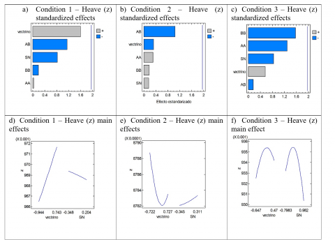
We analyzed the DOE-ANOVA results through the Pareto chart of standardized effects to identify which factor (3DVS = A or SN = B) affected significantly the displacements (surge, sway, heave) of the structure. The factor values were previously normalized and standardized in order to verify if the main effects plots were affected by the modification of the value scales. As a result, there was no evidence homogenizing affected significatively the factors' scales. According to the DOE-ANOVA analysis (Figure 10, Figure 11 and Figure 12) (Table 1), it was observed that run 27 (Condition 3) showed a representative significance level for the sway displacements because of the –AA effect of 3DVS (Figure 11c).
The lateral accelerations of Condition 1 (Figure 11a) and vertical accelerations (Figure 12) showed a positive relationship with the flow velocities measured by 3DVS.
The DOE-ANOVA analysis revealed that the displacements of the floating structure were dominated by the first order-effect of 3DVS (Figure 12a), and second-order effects of 3DVS (AA) (Figure 11a, c), SN (BB) (Figure 10a, Figure 12c). The second-order effect showed an effect with curved main effect plots, which suggests that orbital velocities modulated the variation of the measured waves and currents. Also, the DOE-ANOVA analysis allowed to identify that the floating structure was affected by the near hydrodynamic field measured by 3DVS because of the Sway displacements related to the –AA effects (Figure 11). This –AA effect was the only standardized effect statistically significant, and the associated main effects plot (Figure 11) suggested that the near hydrodynamic field works as a viscous damper with positive relation with the orbital velocities.
Figure 10. Analysis of the fluid-structure interactions from the results of run 9 using the Pareto chart of standardized effects and main effects plots
Figure 11. Analysis of the fluid-structure interactions from the results of run 18 using the Pareto chart of standardized effects and main effects plots
The traditional methods to determine modes and oscillation frequencies work properly during stationary or cyclic loads during dry conditions. These conditions are common for the continental (onshore) structural design, where winds and earthquakes are the main excitation forces. Then, the free vibration and forced tests are performed during stationary conditions, which implies that excitation and response oscillation modes will be harmonic and decreasing. The conditions to determine the offshore structural parameters differ from onshore structures because the load and oscillation modes are not stationary, where the oscillation modes can be linear or non-linear. Because the foundation of an offshore structure is underwater with a damped natural period, water, and soil viscous effects modulate it. Then, the structural natural period and damping parameters should be determined through perturbed and unperturbed forced vibration tests. According to the results of DOE-ANOVA analysis, it is observed that 3DVS properly recorded the near hydrodynamic field; thus, the orbital velocities affected clearly the lateral displacements denoted by the standardized and main effects.
Figure 12. Analysis of the fluid-structure interactions from the results of run 27 using the Pareto chart of standardized effects and main effects plots
Structural parameters such as the natural and damped periods determined by the Logarithmic Decrement and the Half Bandwidth Method showed clear differences during perturbed and unperturbed conditions. The unperturbed structural periods were lower compared to the perturbed structural periods, which revealed the necessity to consider an active damping system for the designing of a floating structure.
The pseudo-acceleration spectra calculated in the near hydrodynamic zone through the 3DVS measurements (Figure 9) were narrowed, lower in the frequency range and higher in peak accelerations (Condition 1 and 2) compared to the pseudo-acceleration spectra (Figure 8) derived from the SN records. However, the damping effect of a constant wind loading over the structure (Condition 3) induced a decrement over the accelerations of 3DVS measurements (Figure 9) and scattered the distribution of the frequency range to lower frequencies, contrary to the pseudo-acceleration spectra from SN measurements which were not affected by the near-damped hydrodynamic field. Then, the structural damping selection differs if the spectra are calculated from velocity records close to the structure or by water level measurements measured in the far field. As a result, the damping coefficient could be mistakenly selected using only one spectrum because the structural amplifications were between 0.0 s and 0.5 s and 0.0 s and 2 s. The pseudo-acceleration spectra result and the structural periods reviewed above justify considering an active damping system for the structure.
The application of the proposed methodology to determine natural and damped periods for a floating offshore structure showed the relevance to consider unperturbed and perturbed conditions for the experimental tests. The Logarithmic Decrement and the Half Bandwidth Method clearly retrieved different structural periods. The Logarithmic Decrement method showed undisturbed damped periods of surge, sway and heave of 1.12 s, 0.7 s and 0.52 s respectively, with damping ratios of 0.047% (surge), 6.167% (sway) and 0.080% (surge). The Half Bandwidth Method reported disturbed damped periods between 0.39 s and 3.76 s for surge (x), 0.49 s and 3.03 s for sway (y) and 0.39 s and 3.85 s for heave (z).
The pseudo-acceleration spectra using free surface accelerations measured through the level sensor (SN), showed peak accelerations between 6.12*10-3 ms-2 and 0.019 ms-2, and the spectra generated through the 3D velocity profiler (3DVS) pointed accelerations between 1.51*10-3 ms-2 and 0.063 ms-2. Hence, the pseudo-acceleration spectra results showed the need to measure loads in the near and far hydrodynamic field because of the variations in magnitude and frequency of the analyzed spectra. As a result, the selection of the damping coefficient and periods to avoid the resonance and structural amplification requires the spectra derived from water level variations measured in the far field and 3D velocity profiles registered in the near hydrodynamic field. The loads on surface were affected by the wave diffraction and reflection what generated a wider pseudo-acceleration spectra.
The DOE-ANOVA analysis showed that the near hydrodynamic field worked as a viscous damper, where the lateral displacements were clearly affected by the orbital velocities measured by the 3DVS. The viscous damping changes the frequency distributions of the pseudo-acceleration spectra and modulates the natural and damped periods of the structure. Thus, an active damping system could deal with the variation of the structural periods because of the waves, wind, and current loads.
The proposed methodology generated transfer function graphs that allowed to identify several amplification peaks and the variations of the frequency ranges. The calculated transfer functions showed the drawbacks of its application due to the non-linearities of the physical processes. As a result, it is necessary to develop new equations and methods for the identification of natural and damped periods which consider the fluid-structure interactions.
Regarding the designing of the floating structure, this research recommends measuring waves, wind and currents in the near and far field on surface and subsurface. Finally, this study recommends future research improving or changing the Half Bandwidth Method for solving the limitations and fails evidenced in this study during the selection of the damping ratios and damped periods.
The authors want to thank the Universidad Militar Nueva Granada, Universidad del Norte, and Universidad Nacional de Colombia sede Medellin for their support in this research through the project IMP-ING-3121.
[1] Rueda-Bayona, J.G., Guzmán, A., Eras, J.J.C., Silva-Casarín, R., Bastidas-Arteaga, E., Horrillo-Caraballo, J. (2019). Renewables energies in Colombia and the opportunity for the offshore wind technology. Journal of Cleaner Production, 220: 529-543. https://doi.org/10.1016/J.JCLEPRO.2019.02.174
[2] Bastidas-Salamanca, M., Bayona, J.G. (2021). Pre-feasibility assessment for identifying locations of new offshore wind projects in the Colombian Caribbean. International Journal of Sustainable Energy Planning and Management, 32: 139-154. https://doi.org/10.5278/IJSEPM.6710
[3] Pokhrel, J., Seo, J. (2019). Natural hazard vulnerability quantification of offshore wind turbine in shallow water. Engineering Structures, 192: 254-263. https://doi.org/10.1016/j.engstruct.2019.05.013
[4] Cruz, A.M., Krausmann, E. (2008). Damage to offshore oil and gas facilities following hurricanes Katrina and Rita: An overview. Journal of Loss Prevention in the Process Industries, 21(6): 620-626. https://doi.org/10.1016/j.jlp.2008.04.008
[5] Hallowell, S.T., Myers, A.T., Arwade, S.R., et al. (2018). Hurricane risk assessment of offshore wind turbines. Renewable Energy, 125: 234-249. https://doi.org/10.1016/J.RENENE.2018.02.090
[6] Atcheson, M., Garrad, A., Cradden, L., Henderson, A., Matha, D., Nichols, J., Sandberg, J. (2016). Floating Offshore Wind Energy. Springer. https://doi.org/10.1007/978-3-319-29398-1
[7] Rueda-Bayona, J.G., Gil, L., Calderón, J.M. (2021). CFD-FEM modeling of a floating foundation under extreme hydrodynamic forces generated by low sea states. Mathematical Modelling of Engineering Problems, 8(6): 888-896. https://doi.org/10.18280/mmep.080607
[8] Gabriel Rueda-Bayona, J., Fernando Osorio-Arias, A., Guzmán, A., Rivillas-Ospina, G. (2019). Alternative method to determine extreme hydrodynamic forces with data limitations for offshore engineering. Journal of Waterway, Port, Coastal, and Ocean Engineering, 145(2): 05018010. https://doi.org/10.1061/(asce)ww.1943-5460.0000499
[9] Jafarabad, A., Kashani, M., Parvar, M.R.A., Golafshani, A.A. (2014). Hybrid damping systems in offshore jacket platforms with float-over deck. Journal of Constructional Steel Research, 98: 178-187. https://doi.org/10.1016/j.jcsr.2014.02.004
[10] Moharrami, M., Tootkaboni, M. (2014). Reducing response of offshore platforms to wave loads using hydrodynamic buoyant mass dampers. Engineering Structures, 81: 162-174. https://doi.org/10.1016/j.engstruct.2014.09.037
[11] Hokmabady, H., Mojtahedi, A., Mohammadyzadeh, S., Ettefagh, M.M. (2019). Structural control of a fixed offshore structure using a new developed tuned liquid column ball gas damper (TLCBGD). Ocean Engineering, 192: 106551. https://doi.org/10.1016/j.oceaneng.2019.106551
[12] Guo, A., Fang, Q., Li, H. (2015). Analytical solution of hurricane wave forces acting on submerged bridge decks. Ocean Engineering, 108: 519-528. https://doi.org/10.1016/j.oceaneng.2015.08.018
[13] Ma, H., Yang, Y., He, Z., Jia, Z., Zhang, Y. (2018). Experimental study on constitutive relation of the high performance marine structural steel under extreme cyclic loads. Ocean Engineering, 168: 204-215. https://doi.org/10.1016/j.oceaneng.2018.09.003
[14] Kandasamy, R., Cui, F., Townsend, N., Foo, C.C., Guo, J., Shenoi, A., Xiong, Y. (2016). A review of vibration control methods for marine offshore structures. Ocean Engineering, 127: 279-297. https://doi.org/10.1016/j.oceaneng.2016.10.001
[15] Ou, J., Long, X., Li, Q.S., Xiao, Y.Q. (2007). Vibration control of steel jacket offshore platform structures with damping isolation systems. Engineering Structures, 29(7): 1525-1538. https://doi.org/10.1016/j.engstruct.2006.08.026
[16] Mojtahedi, A., Yaghin, M.L., Ettefagh, M.M., Hassanzadeh, Y., Fujikubo, M. (2013). Detection of nonlinearity effects in structural integrity monitoring methods for offshore jacket-type structures based on principal component analysis. Marine Structures, 33: 100-119. https://doi.org/10.1016/j.marstruc.2013.04.007
[17] Hosseinlou, F., Mojtahedi, A. (2016). Developing a robust simplified method for structural integrity monitoring of offshore jacket-type platform using recorded dynamic responses. Applied Ocean Research, 56: 107-118. https://doi.org/10.1016/j.apor.2016.01.010
[18] Bajrić, A., Høgsberg, J., Rüdinger, F. (2018). Evaluation of damping estimates by automated operational modal analysis for offshore wind turbine tower vibrations. Renewable Energy, 116: 153-163. https://doi.org/10.1016/j.renene.2017.03.043
[19] Aggarwal, N., Manikandan, R., Saha, N. (2017). Nonlinear short term extreme response of spar type floating offshore wind turbines. Ocean Engineering, 130: 199-209. https://doi.org/10.1016/j.oceaneng.2016.11.062
[20] Marino, E., Giusti, A., Manuel, L. (2017). Offshore wind turbine fatigue loads: The influence of alternative wave modeling for different turbulent and mean winds. Renewable Energy, 102: 157-169. https://doi.org/10.1016/j.renene.2016.10.023
[21] Han, Y., Le, C., Ding, H., Cheng, Z., Zhang, P. (2017). Stability and dynamic response analysis of a submerged tension leg platform for offshore wind turbines. Ocean Engineering, 129: 68-82. https://doi.org/10.1016/j.oceaneng.2016.10.048
[22] Chatziioannou, K., Katsardi, V., Koukouselis, A., Mistakidis, E. (2017). The effect of nonlinear wave-structure and soil-structure interactions in the design of an offshore structure. Marine Structures, 52: 126-152. https://doi.org/10.1016/j.marstruc.2016.11.003
[23] Morató, A., Sriramula, S., Krishnan, N., Nichols, J. (2017). Ultimate loads and response analysis of a monopile supported offshore wind turbine using fully coupled simulation. Renewable Energy, 101: 126-143. https://doi.org/10.1016/j.renene.2016.08.056
[24] Zuo, H., Bi, K., Hao, H. (2017). Using multiple tuned mass dampers to control offshore wind turbine vibrations under multiple hazards. Engineering Structures, 141: 303-315. https://doi.org/10.1016/j.engstruct.2017.03.006
[25] Nielsen, F.G., Hanson, T.D., Skaare, B. (2006). Integrated dynamic analysis of floating offshore wind turbines. In International Conference on Offshore Mechanics and Arctic Engineering, pp. 671-679.
[26] Jonkman, J., Buhl, M. (2007). Development and verification of a fully coupled simulator for offshore wind turbines. In 45th AIAA Aerospace Sciences Meeting and Exhibit, p. 212. https://doi.org/10.2514/6.2007-212
[27] Skaare, B., Hanson, T.D., Nielsen, F.G., Yttervik, R., Hansen, A.M., Thomsen, K., Larsen, T.J. (2007). Integrated dynamic analysis of floating offshore wind turbines. In European Wind Energy Conference and Exhibition, pp. 1929-1939.
[28] Shirzadeh, R., Devriendt, C., Bidakhvidi, M.A., Guillaume, P. (2013). Experimental and computational damping estimation of an offshore wind turbine on a monopile foundation. Journal of Wind Engineering and Industrial Aerodynamics, 120: 96-106. https://doi.org/10.1016/j.jweia.2013.07.004
[29] Subbulakshmi, A., Sundaravadivelu, R. (2016). Heave damping of spar platform for offshore wind turbine with heave plate. Ocean Engineering, 121: 24-36. https://doi.org/10.1016/j.oceaneng.2016.05.009
[30] Wei, K., Myers, A.T., Arwade, S.R. (2017). Dynamic effects in the response of offshore wind turbines supported by jackets under wave loading. Engineering Structures, 142: 36-45. https://doi.org/10.1016/j.engstruct.2017.03.074
[31] Li, M., Zhang, H., Guan, H. (2011). Study of offshore monopile behaviour due to ocean waves. Ocean Engineering, 38(17-18): 1946-1956. https://doi.org/10.1016/j.oceaneng.2011.09.022
[32] Colwell, S., Basu, B. (2009). Tuned liquid column dampers in offshore wind turbines for structural control. Engineering Structures, 31(2): 358-368. https://doi.org/10.1016/j.engstruct.2008.09.001
[33] Shi, W., Park, H., Han, J., Na, S., Kim, C. (2013). A study on the effect of different modeling parameters on the dynamic response of a jacket-type offshore wind turbine in the Korean Southwest Sea. Renewable Energy, 58: 50-59. https://doi.org/10.1016/j.renene.2013.03.010
[34] Chopra, A. (2000). Dynamics of Structures: Theory and Applications to Earthquake Engineering. 2nd ed.
[35] Cruciat, R., Ghindea, C. (2012). Experimental determination of dynamic characteristics of structures. Mathematical Modelling in Civil Engineering, 51-60.
[36] Carswell, W., Johansson, J., Løvholt, F., Arwade, S.R., Madshus, C., DeGroot, D.J., Myers, A.T. (2015). Foundation damping and the dynamics of offshore wind turbine monopiles. Renewable Energy, 80: 724-736. https://doi.org/10.1016/j.renene.2015.02.058
[37] Koukoura, C., Natarajan, A., Vesth, A. (2015). Identification of support structure damping of a full scale offshore wind turbine in normal operation. Renewable Energy, 81: 882-895. https://doi.org/10.1016/j.renene.2015.03.079
[38] Van Der Tempel, J. (2006). Design of Support Structures for Offshore Wind Turbines. https://doi.org/10.2495/978-1-84564-205-1/17
[39] Gavassoni, E., Gonçalves, P.B., de Mesquita Roehl, D. (2015). Nonlinear vibration modes of an offshore articulated tower. Ocean Engineering, 109: 226-242. https://doi.org/10.1016/j.oceaneng.2015.08.028
[40] Segura-Heras, I., Escrivá-Escrivá, G., Alcázar-Ortega, M. (2011). Wind farm electrical power production model for load flow analysis. Renewable Energy, 36(3): 1008-1013. https://doi.org/10.1016/j.renene.2010.09.007
[41] Bhattacharya, S., Lombardi, D., Muir Wood, D. (2011). Similitude relationships for physical modelling of monopile-supported offshore wind turbines. International Journal of Physical Modelling in Geotechnics, 11(2): 58-68. https://doi.org/10.1680/ijpmg.2011.11.2.58
[42] Bhattacharya, S., Nikitas, N., Garnsey, J., et al. (2013). Observed dynamic soil–structure interaction in scale testing of offshore wind turbine foundations. Soil Dynamics and Earthquake Engineering, 54: 47-60. https://doi.org/10.1016/j.soildyn.2013.07.012
[43] Chakrabarti, S. (1998). Physical model testing of floating offshore structures. In Dynamic Positioning Conference, pp. 1-33.
[44] Otter, A., Murphy, J., Pakrashi, V., Robertson, A., Desmond, C. (2022). A review of modelling techniques for floating offshore wind turbines. Wind Energy, 25(5): 831-857. https://doi.org/10.1002/WE.2701
[45] Montgomery, D.C. (2017). Design and Analysis of Experiments. Ninth Edit. Hoboken, NJ, USA: John Wiley & Sons, Inc.
[46] Chakrabarti, S.K. (2015). Chapter 13 Physical Modelling of Offshore Structures. Elsevier Ltd. https://doi.org/10.1016/B978-0-08-044381-2.50020-5
[47] NWS-NOAA. (2020). Saffir-Simpson Hurricane Wind Scale 2020. https://www.weather.gov/mfl/saffirsimpson, accessed on June 3, 2020.
[48] Power, H. E., Gharabaghi, B., Bonakdari, H., Robertson, B., Atkinson, A. L., Baldock, T.E. (2019). Prediction of wave runup on beaches using Gene-Expression Programming and empirical relationships. Coastal Engineering, 144: 47-61. https://doi.org/10.1016/j.coastaleng.2018.10.006
[49] Derschum, C., Nistor, I., Stolle, J., Goseberg, N. (2018). Debris impact under extreme hydrodynamic conditions part 1: Hydrodynamics and impact geometry. Coastal Engineering, 141: 24-35. https://doi.org/10.1016/j.coastaleng.2018.08.016
[50] Hanley, M.E., Hoggart, S.P.G., Simmonds, D.J., et al. (2014). Shifting sands? Coastal protection by sand banks, beaches and dunes. Coastal Engineering, 87: 136-146. https://doi.org/10.1016/j.coastaleng.2013.10.020
[51] Rueda-Bayona, J.G., Guzmán, A., Cabello Eras, J.J. (2020). Selection of JONSWAP spectra parameters during water-depth and sea-state transitions. Journal of Waterway, Port, Coastal and Ocean Engineering, 6: 14. https://doi.org/10.1061/(ASCE)WW.1943-5460.0000601
[52] Qiao, C., Myers, A.T., Arwade, S.R. (2020). Characteristics of hurricane-induced wind, wave, and storm surge maxima along the US Atlantic coast. Renewable Energy, 150: 712-721. https://doi.org/10.1016/j.renene.2020.01.030
[53] Amirinia, G., Jung, S. (2017). Buffeting response analysis of offshore wind turbines subjected to hurricanes. Ocean Engineering, 141: 1-11. https://doi.org/10.1016/j.oceaneng.2017.06.005