Lalaoui Lahouaoui* | Djaalab Abdelhak | Bendjaafer Abderrahmane | Meddah Toufik
© 2022 IIETA. This article is published by IIETA and is licensed under the CC BY 4.0 license (http://creativecommons.org/licenses/by/4.0/).
OPEN ACCESS
This article reviews the field of image processing in recent years is enormously developed and it has been used in several specialties like medical, stand-alone, satellite and the purpose of this field is to improve image quality and extract information. Pneumonia has become in recent years a defective disease that affects the majorities of the population is especially the elderly and can sometimes put their lives in danger, in order to save human life early pneumonia diagnostic is necessary; in this work we have based on the detection and classification of patients with pneumonia from their chest x-ray. However, there are several areas where image classification is applied with success, in our work we have used deep learning based on the most common convolutional neural networks to make an image classification of pneumonia disease and to obtained good results and gave several advantages.
images classification, convolution neural networks, deep learning, evaluation criteria
The field of image processing in recent years is enormously developed and it has been used in several specialties like medical, stand-alone, satellite and the purpose of this field is to improve image quality and extract information. Automatic retrieval, analysis and understanding of useful information from a single image or image sequence. Recent research has attracted a great deal of attention from in-depth learning methods, especially convolutional neural networks (CNN) [1, 2]. Compared to the SVM methods, CNN can operate the original data without transformation and keep the information in the original data as much as possible we have need methods like SVM and CNN. We used convolutional neural networks (CNN) for automatic image classification. Pneumonia has become in recent years a defective disease that affects the majorities of the population is especially the elderly and can sometimes put their lives in danger, in order to save human life early pneumonia diagnostic is necessary; in this work we have based on the detection and classification of patients with pneumonia from their chest x-ray. Very recently, deep learning is of interest to researchers in the field of computer vision. In particular, convolutional neural networks (CNNs) have attracted a lot of attention due to their superior performance in many domains, such as face recognition [3-5], object detection and video classification [6-8].
Application areas for learning multiple functionalities are computer vision [9] pedestrian detection [10] and multimedia research [11]. However, there are several areas where image classification is applied with success, in our work we have used deep learning based on the most common convolutional neural networks to make an image classification of pneumonia disease and to obtained good results and gave several advantages. The CNN network with its pooling layer allows a better recognition force for images that are slightly translated. The CNN requires each image to pass through the convolution, pooling and activation function layers, which is only based on the automatic extraction of high-level parameters. In addition, the number of network layers and other hyper-parameters, by adjusting the size of the convolution core, it is efficient to extract features of different levels, which is more efficient than other methods. Zhang et al. [12] proposed an underwater classification method based on a neural network of self-organized characteristic maps. However, for specific subjects it is not possible to use CNN directly by what can cause problem. Therefore, in 2016, an effective approach was proposed to learning a rotation invariant CNN model to improve object detection, which is achieved through the introduction and learning of a new rotation-invariant layer based on existing CNN architectures [13, 14]. In addition, the study [15] suggested the scene classification based on new feature representation method that generates visual words from deep convolutional features using standard NCN. In addition, a new, simple but effective method for learning discriminatory CNs is proposed to solve the problems of diversity within the classroom and similarity between classes and to improve the performance of the classification of image scenes in remote sensing [16]. Resolution of the CNN problem and improved classification performance for various datasets by sharing convolution method weights [17, 18]. The use of an effective deep learning algorithm, Contrastive Divergence (CD), in which each layer is formed layer by layer is the fascinating performance revolution of the deep belief nets according to Bruyndonckx et al. [19]. Those features can be used to guide medical interventions and in radiotherapy in particular [20].
The remainder of paper is organized as follows: the different methods for classification was presented in section 2; in section 3 we presented the results of simulation and finally, discuss resultants with perspective and conclude this article, respectively.
Image classification consists in labeling the constituent elements of an image according to a predefined rule. It involves the use of an algorithm that assigns labels to groups of pixels or vectors. Image classification is a process of computer vision, and in particular the most important step of this technology. Two general methods classification are "supervised" and "unsupervised".
The goal of image classification is to develop a system capable of automatically assigning a class to an image. Thus, this system makes it possible to carry out an expert task which can be expensive to acquire for a human being due in particular to physical constraints such as concentration, fatigue or the time required by a volume of image data [21].
Binary classification consists of classifying a set of data or images into two classes using a classifier, is widely used in many fields, this section covers many algorithms widely used for binary classification. Each algorithm has its advantages and disadvantages and some algorithms are suitable for certain applications.
2.1 Classification methods
2.1.1 Supervised methods
The purpose of supervised classification is primarily to define rules for classifying objects into classes from qualitative or quantitative variables characterizing these objects. Methods often extend to Y variables quantitative (regression). there are the most important algorithms in supervised learning: (1) K-Means; (2) Logistic regressions; (3) Support vector machines (SVM); (4) Neural networks.
2.1.2 Unsupervised methods
The purpose of classification is to group (partition, segment) not observations into a certain number of homogeneous groups or classes. There are two main types of classification: supervised classification, often simply called classification (Classification in English); unsupervised classification, sometimes called partitioning, segmentation or clustering [22].
The most important algorithms in unsupervised learning are: (1) K-Means; (2) Fuzzy C-means, as presented in Figure 1.
Figure 1. Difference between a) supervised learning and b) unsupervised learning
2.2 Performance measures for classification
2.2.1 Confusion matrix
Is a tool for measuring the performance of a Machine Learning model by checking in particular how often its predictions are accurate compared to reality in classification problems.
To fully understand how a confusion matrix works, it is important to understand the four main terminologies: TP, TN, FP and FN (Table 1).
Table 1. Matrice de confusion
|
Response expert |
P |
N |
|
|
Response classifier |
Y |
True Positive |
false Positive |
|
N |
Faux Negative |
True Negative |
|
True positive TP: Correctly predicted Class 1 element. True negative TN: Correctly predicted class 0 element. False positive FP: Poorly predicted Class 1 element. False negative FN: Class 0 element poorly predicted.
It is possible to calculate several indicators summarizing the confusion matrix:
(1) Accuracy
Closeness of agreement between the test result and the reference value accepted:
Accuracy $=\frac{(\mathrm{TP}+\mathrm{FN})}{(\mathrm{TP}+\mathrm{TF}+\mathrm{FP}+\mathrm{FN})}$ (1)
(2) Precision
It indicates the accuracy of the model in terms of positive predictions.
precision $=\frac{(\mathrm{TP})}{(\mathrm{TP}+\mathrm{FP})}$ (2)
(3) Recall
Mathematical comparison, recall is defined as follows:
Recall $=\frac{(T P)}{(T P+F N)}$ (3)
(4) F1 Score
It gives a balance between accuracy and recall.
$F 1=2 \star \frac{\text { Precision }-\text { Recall }}{\text { Precision }+\text { Recall }}$ (4)
(5) Sensitivity
Sensitivity or True Positive Rate (TPR).
Sensitivity $=\frac{(T P)}{(T P+F N)}$ (5)
(6) Specificity
Specificity (SPC) or True Negative Rate (TNR).
Specificity $=\frac{T N}{(\text { FP }+T N)}$ (6)
2.2.2 Curve of ROC
The ROC (Receiver Operating Characteristic) curve represents the sensitivity as a function of 1 – specificity for all possible threshold values of the marker studied. Sensitivity is the ability of the test to detect patients well and specificity is the ability of the test to detect non-patients well [23]. The ROC curve is that each point of this curve predicts the accuracy of the model. Figure 2 presented the curve ROC.
Figure 2. Curve of ROC
2.3 Convolutional neural networks
The difference between Artificial Neural Networks (ANN) and Convolutional Neural Networks (CNN) ANN uses weights and an activation function for the bulk of its method. The “layers” in ANN are rows of data points hosted through neurons that all use the same neural network. ANN uses weights to learn. Weights get changed after each iteration through the neuron in ANN. ANN goes back and changes the weights depending on the accuracy calculated by a “cost function”.
There is no neuron or weights in CNN. CNN instead casts multiple layers on images and uses filtration to analyze image inputs. These layers are the math layer, rectified linear unit layer, and fully connected layer. ANN processes inputs in a different way than CNN. As a result, ANN is sometimes referred to as a Feed-Forward Neural Network because inputs are processed only in a forward-facing direction.
Convolutional neural networks have a similar methodology to traditional supervised learning methods: they receive input images, detect the features of each of them, and then train a classifier on them. However, features are learned automatically! CNN does all the tedious work of feature extraction and description itself:
During the training phase, the classification error is minimized in order to optimize the parameters of the classifier.
This CNN code at the output of the convolutional part is then connected to the input of a second part, consisting of fully connected layers (multilayer perceptron). The role of this part is to combine the characteristics of the CNN code to classify the image. The output is a final layer with one neuron per category. The numerical values obtained are usually normalized between 0 and 1, summing to 1, to produce a probability distribution over the categories.
Convolutional networks are a special form of multi-layered neural networks. Convolutional neural networks (also called CNNs) are characterized by their first convolutional layers (usually one to three). A convolutional layer is based on the mathematical principle of convolution, and seeks to identify the presence of a pattern (most often in an image, or a signal) [24].
The first part of a CNN is the convolutional part itself. It works as an image feature extractor. An image is passed through a succession of filters, or convolution cores, creating new images called convolution maps. Some intermediate filters reduce the resolution of the image by a local maximum operation. In the end, the convolution maps are flattened and concatenated into a characteristic vector, called the CNN code. This CNN code at the output of the convolutive part is then connected as the input of a second part, consisting of fully connected layers (multilayer perceptron). The role of this part is to combine the characteristics of the CNN code to classify the image. The output is a final layer with one neuron per category. The numerical values obtained are generally normalized between 0 and 1, of sum 1, to produce a probability distribution on categories.
Convolutional neural networks have many applications in image recognition, video recognition or natural language processing [25-27].
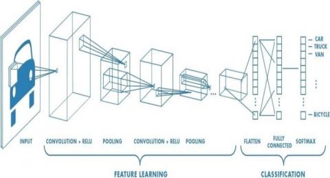
Convolutional neural networks have two distinct parts, a first part which we call the convolutional part of the model and the second part, which we will call the classification part.
Figure 3 shows the architecture convolutional neural network.
Figure 3. Architecture convolutional neural network
2.4 The convolutional layer
A convolution layer is a fully connected (FC) layer, i.e. all neurons in the previous layer are connected to all neurons in this layer.
The convolution layer is the key component of convolutional neural networks, and is always at least their first layer.
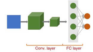
Its purpose is to identify the presence of a set of features in the images received as input. To do this, a convolution filtering is carried out: the principle is to "slide" a window representing the feature over the image, and to calculate the convolution product between the feature and each portion of the scanned image. A feature is then seen as a filter: the two terms are equivalent in this context. Figure 4 describes the convolutional with multiple filters.
Figure 4. Convolutional with multiple filters [28]
2.5 Fully connected layer and loss layer
This layer is at the end of the network. It allows the classification of the image from the characteristics extracted by the succession of processing blocks. It is entirely connected, because all the inputs of the layer are connected to the output neurons of this one. They have access to all input information. Each neuron assigns to the image a probability value of belonging to class i among the C possible classes [28].
The loss layer is the last layer of the network. It calculates the error between the network forecast and the actual value. During a classification task, the random variable is discrete, because it can only take the values 0 or 1, representing membership (1) or not (0) in a class. This is why the most common and suitable loss function is the cross-entropy function [29].
2.6 Auto encoders
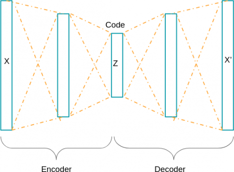
Autoencoders are somewhat special neural networks that have exactly the same number of neurons on their input layer and their output layer. The goal for an autoencoder is to have an output closest to the input! The learning is therefore “self-supervised” because the loss to be minimized is the reconstruction cost between the output and the input. The data therefore does not have to be labeled, because it is its own label, which therefore makes this model an unsupervised model [30-32].
The architecture of our network is presented in Figure 5:
Figure 5. Image shown auto encoder
2.7 Improved neural network performance
There are several techniques to improve the performance of neural networks, because initially this performance can often be unsatisfactory, the main conceptual factors causing the performance degradation are the problem of over-learning and the wrong choice of hyper parameters. We have selected some performance improvement techniques to test them on our model [33, 34].
2.8 Proposed architecture
The proposed CNN model has a global architecture which consists of two main parts [35]:
(a) Parameter extraction.
(b) Classifier.
For each layer of the feature extraction layer their input is the output of the immediately preceding layers, and its output is passed to the inputs of the following layers.
In Figure 6 we presented the proposed architecture consists of the layers of convolutional, max pooling and classification combined together.
Feature extractors include 3×3, 256 convolutional layers; 3×3, 64; 3×3, 16, a max-pooling layer of size 2×2, and a Rectified Linear Unit (RELU) activator between them.
The outputs of convolutional max-pooling operations are assembled into 2 drop outs of size 0.5, two dense layers of size 64 and 1 respectively. A RELU between the two dense layers and a sigmoid activation function that performs task classification. There are three convolutional layers with the same number of Maxpooling layers followed by flat layers, same number of Maxpooling layers, followed by the zero parameter flatten layer and dense layers of about 10,000 parameters.
So, the total of trainable parameters in the network comes to 799791.00 parameters, this summary of the model gives quick information about the deep neural network. Figure 6 presents the proposed architecture.
Figure 6. Proposed architecture
Pneumonia is one of the most dangerous diseases, it is an infectious disease that affects the lungs and threatens human life. It is usually caused by bacteria called Streptococcus pneumonia as documented in 2017; it is dangerous because it kills about a hundred million people a year. Early diagnosis of pneumonia is of paramount importance to save the lives of many people.
For reasons of their performance in image processing, deep learning algorithms (CNNs) have attracted a lot of attention for classification, and our work is aimed at detecting and classifying patients with pneumonia based on chest x-ray images.
The statistical results obtained demonstrate that pre-trained CNN models used with supervised classification algorithms can be of great benefit in analyzing chest x-rays, especially in detecting pneumonia.
3.1 Materials and methods
We present the detailed experiments and evaluation steps undertaken to test the effectiveness of the proposed model; our experiments were based on a chest x-ray image dataset proposed in Ref. [35].
All experiments were performed on an HP PC the high game.
3.2 Data BASES
The diagnoses we used in the database are based on a set of chest X-rays published on the Kaggle website, all images are composite x-rays made up of the RGB format, the open-source deep learning framework Keras with the Tensor Flow backend is used to build and train the Build and train the convolutional neural network.
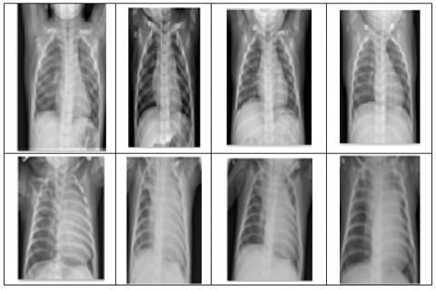
We obtained a synthesis of images such as learning images and test and validation images; each of them is devised by pneumonia and normal chest x-rays; the data obtained is intended to improve and increase without efficiency, a total of approximately 5,216 it can be noticed that the majority of the images in the training and likewise, a total of 624 images are allocated to the validation in order to improve the overall accuracy. Figure 7 shows the X-ray sample without pneumonia.
Figure 7. X-ray sample without pneumonia
3.3 Pretreatment and augmentation
The goal is to use data augmentation methods that involve artificially increasing the size and quality of the dataset, this process resolves over fitting issues and improves the generalizability of the model during training. The parameters deployed in the augmentation of images are shown below in (Table 2).
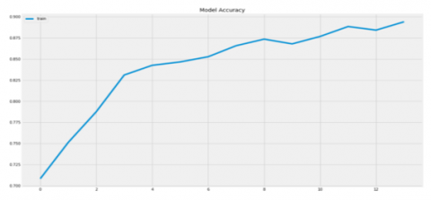
The following figures show the learning results of the proposed architecture. Figure 8 presents the Precision models.
Figure 9 represents the precision in the training step from the database used.
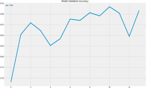
The model precision validation is shown in Figure 10.
Table 2. Settings for image enhancement
|
Layers |
Output form |
Parameter |
|
CONV2D |
(NONE, 200, 200, 256) |
2560 |
|
ACTIVATION |
(NONE, 200, 200, 256) |
0 |
|
MAX_POOLING2D |
(NONE, 100, 100, 256) |
0 |
|
BATCH_NORMALIZ |
(NONE, 100, 100, 256) |
400 |
|
CONV2D_1 |
(NONE, 100, 100, 64) |
147520 |
|
ACTIVATION_1 |
(NONE, 100, 100, 64) |
0 |
|
MAX_POOLING2D_1 |
(NONE, 50, 50, 64) |
0 |
|
BATCH_NORMALIZ_1 |
(NONE, 50, 50, 64) |
200 |
|
CONV2D_2 |
(NONE, 50, 50, 16) |
9232 |
|
ACTIVATION_2 |
(NONE, 50, 50, 16) |
0 |
|
MAX_POOLING2D_2 |
(NONE, 25, 25, 16) |
0 |
|
BATCH_NORMALIZ_2 |
(NONE, 25, 25, 16) |
100 |
|
FLATTEN |
(NONE, 10000) |
0 |
|
DROPOUT |
(NONE, 10000) |
0 |
|
DENSE |
(NONE, 64) |
640064 |
|
ACTIVATION_3 |
(NONE, 64) |
0 |
|
DROPOUT_1 |
(NONE, 64) |
0 |
|
DENSE_1 |
(NONE, 1) |
65 |
|
ACTIVATION_4 |
(NONE, 1) |
0 |
|
Total params |
800,141 |
|
|
Trainable params |
799,791 |
|
|
Non-trainable params |
350 |
|
Figure 8. Precision models
Figure 9. Model loss
Figure 10. Model precision validation
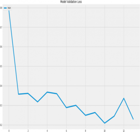
Figure 11. Model loss validation
Figure 11 shows the deterioration of the loss which is what we want in our study. The proposed networks are test and evaluate their performance, the parameters and hyper parameters were set during training; Figures 12 shows the training accuracy and training loss curves obtained during training.
Models for 15 eras. The learning accuracy of the model at 91.63%, and the learning loss of the model at 0.1997, and a corresponding accuracy of 91.14% and 0.2282 loss for validation. an important and deep convolutional neural network gives good results and the performance of our network degrades if a convolutional layer is removed. The following Table 3 represents the different results obtained.
Table 3. Result of the proposed CNN architecture
|
Threshold |
0.86 |
0.84 |
0.80 |
0.75 |
0.73 |
0.70 |
0.65 |
0.50 |
|
Accuracy |
0.91 |
0.91 |
0.91 |
0.90 |
0.90 |
0.89 |
0.86 |
0.73 |
|
Precision |
0.83 |
0.86 |
0.89 |
0.93 |
0.94 |
0.96 |
0.97 |
0.99 |
|
Recall |
0.87 |
0.84 |
0.82 |
0.78 |
0.77 |
0.74 |
0.67 |
0.51 |
|
F1 score |
0.85 |
0.85 |
0.85 |
0.85 |
0.85 |
0.84 |
0.79 |
0.67 |
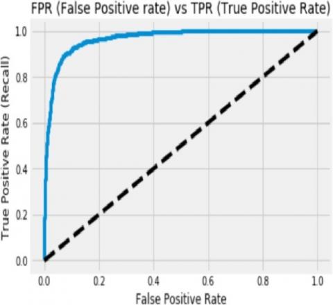
Figure 12. ROC curve of our result
In Figure 12, it shows the Roc of curve between the true positive rate and false positive rate.
In the phase of the prediction, we found the results in the Table 4:
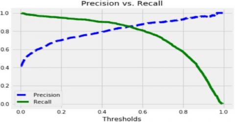
From (Table 4), we can conclude that for the threshold equal to 0.5 we find a high precision value and small values for the other criteria. And for the threshold value equal to 0.86 we notice that a bad precision value and better values for the other criteria.
The Precision vs. Recall is presented in Figure 13.
Table 4. Results in the prediction phase
|
Period |
Accuracy of training |
Loss of training |
Accuracy of validation |
Loss of validation |
|
1 |
0.7120 |
0.6431 |
0.7407 |
0.6431 |
|
3 |
0.8044 |
0.4152 |
0.7940 |
0.3886 |
|
5 |
0.8489 |
0.3489 |
0.8549 |
0.3175 |
|
10 |
0.8740 |
0.2899 |
0.9114 |
0.2183 |
|
12 |
0.8793 |
0.2795 |
0.9146 |
0.2160 |
|
15 |
0.8887 |
0.2651 |
0.8943 |
0.2466 |
Figure 13. Image Represented Precision vs. Recall
We have introduced the convolutional neural networks by presenting the different types of layers used in the classification: the convolutional layer, the grinding layer, the pooling and the fully connected layer. The use of CNNs is given good results to classify the disease of pneumonia, using a database contains images of people (sick / not sick) in order to detect the presence of the disease more quickly and accurately. In this work we have discussed the fundamentals of image classification and Deep Learning based on convolutional neural networks in particular. We introduced these convolutional neural networks by presenting the different types of layers used in the classification: The convolutional layer, the Relu layer, the pooling layer and the fully connected layer, we also talked about the regularization methods (dropout and data increase, early stopping, learning rate, batch normalization, etc.…) used to avoid the problem of over learning. Has end to solve the classification problems to detect pneumonia disease. According to the results that obtained through the quantitative metric values which demonstrate for researchers to change the architectures of the proposed method to improve the metric values. Convolutional Neural networks (CNN) have great performance while classifying images which are very similar to the dataset. For future technology development I propose to classify images 3D with fully CNN, if images contain some degree of tilt or rotation then CNNs usually have difficulty in classifying the image.
The present work was used, the database is based on a set of chest X-rays published on the Kaggle website, all images are composite x-rays made up of the RGB format, and the open-source deep learning framework Keras with the Tensor Flow backend is used to build and train the Build and train the convolutional neural network.
[1] Currie, G., Hawk, K.E., Rohren, E., Vial, A., Klein, R. (2019). Machine learning and deep learning in medical imaging: Intelligent imaging. Journal of Medical Imaging and Radiation Sciences, 50(4): 477-487. https://doi.org/10.1016/j.jmir.2019.09.005
[2] Kayalibay, B., Jensen, G., van der Smagt, P. (2017). CNN-based segmentation of medical imaging data. arXiv preprint arXiv:1701.03056. https://doi.org/10.48550/arXiv.1701.03056
[3] Li, J., Qiu, T., Wen, C., Xie, K., Wen, F.Q. (2018). Robust face recognition using the deep C2D-CNN model based on decision-level fusion. Sensors, 18(7): 2080. https://doi.org/10.1155/2020/8861987
[4] Shao, H., Chen, S., Zhao, J.Y., Cui, W.C., Yu, T.S. (2015). Face recognition based on subset selection via metric learning on manifold. Frontiers of Information Technology & Electronic Engineering, 16(12): 1046-1058. https://doi.org/10.1631/FITEE.1500085
[5] Madhavan, S., Kumar, N. (2021). Incremental methods in face recognition: A survey. Artificial Intelligence Review, 54(1): 253-303. https://doi.org/10.1007/s10462-019-09734-3
[6] Shen, Z., Liu, Z., Li, J., Jiang, Y. G., Chen, Y., Xue, X. (2017). DSOD: Learning deeply supervised object detectors from scratch. In Proceedings of the IEEE International Conference on Computer Vision, pp. 1919-1927. https://doi.org/10.48550/arXiv.1708.01241
[7] Tian, Z., Shen, C., Chen, H., He, T. (2019). Fcos: Fully convolutional one-stage object detection. In Proceedings of the IEEE/CVF International Conference on Computer Vision, pp. 9627-9636. https://doi.org/10.48550/arXiv.1904.01355
[8] Zhao, Q., Sheng, T., Wang, Y., Tang, Z., Chen, Y., Cai, L., Ling, H. (2019). M2det: A single-shot object detector based on multi-level feature pyramid network. In Proceedings of the AAAI Conference on Artificial Intelligence, 33(1): 9259-9266. https://doi.org/10.1609/aaai.v33i01.33019259
[9] Chaquet, J.M., Carmona, E.J., Fernández-Caballero, A. (2013). A survey of video datasets for human action and activity recognition. Computer Vision and Image Understanding, 117(6): 633-659. http://dx.doi.org/10.1016/j.cviu.2013.01.01
[10] Dhiman, C., Vishwakarma, D.K. (2019). A review of state-of-the-art techniques for abnormal human activity recognition. Engineering Applications of Artificial Intelligence, 77: 21-45. http://dx.doi.org/10.1016/j.engappai.2018.08.014
[11] Mademlis, I., Tefas, A., Pitas, I. (2019). Greedy salient dictionary learning for activity video summarization. In International Conference on Multimedia Modeling, pp. 578-589. http://dx.doi.org/10.1007/978-3-030-05710-7_48
[12] Zhang, Z., Yan, S., Zhao, M. (2014). Similarity preserving low-rank representation for enhanced data representation and effective subspace learning. Neural Networks, 53: 81-94. http://dx.doi.org/10.1016/j.neunet.2014.01.001
[13] Girshick, R., Donahue, J., Darrell, T., Malik, J. (2015). Region-based convolutional networks for accurate object detection and segmentation. IEEE Transactions on Pattern Analysis and Machine Intelligence, 38(1): 142-158. http://dx.doi.org/10.1109/TPAMI.2015.2437384
[14] Van Ginneken, B., Setio, A.A., Jacobs, C., Ciompi, F. (2015). Off-the-shelf convolutional neural network features for pulmonary nodule detection in computed tomography scans. In 2015 IEEE 12th International Symposium on Biomedical Imaging (ISBI), pp. 286-289. http://dx.doi.org/10.1109/ISBI.2015.7163869
[15] Shen, W., Zhou, M., Yang, F., Yang, C., Tian, J. (2015). Multi-scale convolutional neural networks for lung nodule classification. In International Conference on Information Processing in Medical Imaging, pp. 588-599. http://dx.doi.org/10.1007/978-3-319-19992-4_46
[16] Shi, C., Zhang, X., Sun, J., Wang, L. (2021). Remote sensing scene image classification based on dense fusion of multi-level features. Remote Sensing, 13(21): 4379. https://doi.org/10.3390/rs13214379
[17] Dhillon, A., Verma, G.K. (2020). Convolutional neural network: A review of models, methodologies and applications to object detection. Progress in Artificial Intelligence, 9(2): 85-112. https://doi.org/10.1007/s13748-019-00203-0
[18] Lee, H., Grosse, R., Ranganath, R., Ng, A.Y. (2009, June). Convolutional deep belief networks for scalable unsupervised learning of hierarchical representations. In Proceedings of the 26th Annual International Conference on Machine Learning, pp. 609-616. https://doi.org/10.1145/1553374.1553453
[19] Bruyndonckx, P., Lemaitre, C., Van Der Laan, D.J., et al. (2008). Evaluation of machine learning algorithms for localization of photons in undivided scintillator blocks for PET detectors. IEEE Transactions on Nuclear Science, 55(3): 918-924. https://doi.org/10.1109/TNS.2008.922811
[20] Ravì, D., Wong, C., Deligianni, F., Berthelot, M., Andreu-Perez, J., Lo, B., Yang, G.Z. (2016). Deep learning for health informatics. IEEE Journal of Biomedical and Health Informatics, 21(1): 4-21. https://doi.org/10.1109/JBHI.2016.2636665
[21] Yamashita, R., Nishio, M., Do, R.K.G., Togashi, K. (2018). Convolutional neural networks: An overview and application in radiology. Insights into Imaging, 9(4): 611-629. https://doi.org/10.1007/s13244-018-0639-9
[22] Sahiner, B., Pezeshk, A., Hadjiiski, L.M., et al. (2019). Deep learning in medical imaging and radiation therapy. Medical Physics, 46(1): e1-e36. https://doi.org/10.1002/mp.13264
[23] Litjens, G., Kooi, T., Bejnordi, B.E., et al. (2017). A survey on deep learning in medical image analysis. Medical Image Analysis, 42: 60-88. https://doi.org/10.1016/j.media.2017.07.005
[24] Schmitz, R., Madesta, F., Nielsen, M., Krause, J., Steurer, S., Werner, R., Rösch, T. (2021). Multi-scale fully convolutional neural networks for histopathology image segmentation: From nuclear aberrations to the global tissue architecture. Medical Image Analysis, 70: 101996. https://doi.org/10.1016/j.media.2021.101996
[25] Ali, R., Chuah, J.H., Talip, M.S.A., Mokhtar, N., Shoaib, M.A. (2021). Automatic pixel-level crack segmentation in images using fully convolutional neural network based on residual blocks and pixel local weights. Engineering Applications of Artificial Intelligence, 104: 104391. https://doi.org/10.1016/j.engappai.2021.104391
[26] Jiang, W., Ren, Y., Liu, Y., Leng, J. (2021). A method of radar target detection based on convolutional neural network. Neural Computing and Applications, 33(16): 9835-9847. https://doi.org/10.1007/s00521-021-05753-w
[27] Chen, L.C., Papandreou, G., Kokkinos, I., Murphy, K., Yuille, A.L. (2017). Deeplab: Semantic image segmentation with deep convolutional nets, atrous convolution, and fully connected CRFS. IEEE Transactions on Pattern Analysis and Machine Intelligence, 40(4): 834-848. https://doi.org/10.48550/arXiv.1606.00915
[28] Çiçek, Ö., Abdulkadir, A., Lienkamp, S.S., Brox, T., Ronneberger, O. (2016). 3D U-Net: Learning dense volumetric segmentation from sparse annotation. In International Conference on Medical Image Computing and Computer-Assisted Intervention, pp. 424-432. https://doi.org/10.1007/978-3-319-46723-8_49
[29] Karacı, A. (2022). VGGCOV19-NET: Automatic detection of COVID-19 cases from X-ray images using modified VGG19 CNN architecture and YOLO algorithm. Neural Computing and Applications, pp. 1-22. https://doi.org/10.1007/s00521-022-06918-x
[30] Ahmed, E., Saint, A., Shabayek, A.E.R., Cherenkova, K., Das, R., Gusev, G., Aouada, D., Ottersten, B. (2018). A survey on deep learning advances on different 3D data representations. arXiv preprint arXiv:1808.01462. https://doi.org/10.48550/arXiv.1808.01462
[31] Ravì, D., Wong, C., Deligianni, F., Berthelot, M., Andreu-Perez, J., Lo, B., Yang, G.Z. (2016). Deep learning for health informatics. IEEE Journal of Biomedical and Health Informatics, 21(1): 4-21. https://doi.org/10.1109/JBHI.2016.2636665
[32] Sakas, G. (2002). Trends in medical imaging: From 2D to 3D. Computers & Graphics, 26(4): 577-587. https://doi.org/10.1016/S0097-8493(02)00103-6
[33] Wang, L., Lee, C.Y., Tu, Z., Lazebnik, S. (2015). Training deeper convolutional networks with deep supervision. arXiv preprint arXiv:1505.02496. https://doi.org/10.48550/arXiv.1505.02496
[34] Ker, J., Wang, L., Rao, J., Lim, T. (2017). Deep learning applications in medical image analysis. IEEE Access, 6: 9375-9389. https://doi.org/10.1109/ACCESS.2017.2788044
[35] https://www.kaggle.com/paultimothymooney/chest-xray-pneumonia, accessed on October 18, 2021.