Duc Ngoc Nguyen | Tuan Anh Nguyen* | Ngoc Duyen Dang | Thi Thu Huong Tran | Thang Binh Hoang
© 2022 IIETA. This article is published by IIETA and is licensed under the CC BY 4.0 license (http://creativecommons.org/licenses/by/4.0/).
OPEN ACCESS
The suspension system plays a role in ensuring the stability of the vehicle when traveling on the road. On many modern vehicles, the active suspension system has been proposed to replace the conventional passive suspension system. The performance of the controller for the active suspension system depends on its control method. In this paper, a half dynamics model of the vehicle is established. Besides, the LQR control method is also used. The parameters of the control matrix are calculated through the triple in-loop optimization algorithm, which has been shown in the research. This is a completely novel algorithm. This algorithm helps to choose the most optimal parameters. Thus, it ensures the efficiency and stability of the controller. The calculation and comparison process are done automatically. When the loop ends, the optimal parameters are explicitly indicated. The simulation process is done in the MATLAB-Simulink environment. The results of the research showed that when the LQR controller, which was optimized through the triple in-loop algorithm used, the vehicle's oscillation was significantly reduced. In the three survey situations, the values of the roll angle and the angular acceleration of the sprung mass are guaranteed to be stable. Besides, when using this controller, the phenomenon of “chattering” after the excitation ends does not appear. This topic can be further developed in the future.
active suspension system, LQR controller, triple in-loops algorithm
1.1 Oscillation of the vehicle
The oscillation of the vehicle is one of the important issues. It can affect the stability and smoothness of the vehicle. Besides, the problems of oscillation are also related to the durability and longevity of the vehicle. There are many causes of oscillation, in which, the stimulation from the road surface is the direct cause of this phenomenon.
The suspension system is an important part of the vehicle, and it helps to regulate and extinguish the oscillations transmitted from the road surface to the vehicle body. Normally, the suspension system will consist of three elements corresponding to their three functions: the elastic element (spring, leaf spring), the oscillation damping element (damper), and the guiding element (lever arm). The suspension system separates the vehicle into two parts. All assemblies located above the suspension are called sprung masses. In contrast, what lies below the suspension system is known as the un-sprung mass. These masses have a great influence on the vehicle's oscillation [1]. In today's popular vehicles, passive suspension (mechanical) is often used. For this suspension system, the stiffness of the spring and damper is unchanged. Therefore, in many special cases, the smoothness and comfort of the vehicle may not be guaranteed. To improve the system’s instability, several modern suspension systems that are controlled automatically have been proposed. On some high-end models, the air suspension system has been equipped. For this system, the stiffness of the air spring can be changed continuously. This change depends on the traveling conditions of the vehicle [2, 3]. Thus, the smoothness can be enhanced. In addition, the damping coefficient can also be changed through the semi-active suspension. Inside the electronic damper, extremely small iron filings are arranged through a magnetic field, which is generated by the current supplied from the controller [4-6]. Besides, the active suspension system, which uses hydraulic actuators, was introduced, and used on some luxury models [7, 8]. The effect the active suspension system brings is very positive, and the vehicle's oscillations can be significantly improved.
In some research about vehicle oscillation, the quarter dynamics and half dynamics models are often used. For the quarter dynamics model, it describes the vehicle's oscillation through a position of a suspension system. It is quite simple. The oscillation criteria in this model include displacement and acceleration of the sprung mass. However, this model cannot completely describe the effects of the oscillation on the vehicle. Therefore, the half dynamics model is used to replace the other model. The half dynamics model describes the vehicle's oscillations through the two sides of the suspension system. In this model, the roll angle was taken into consideration. The oscillation criteria can be the vertical displacement and acceleration of the sprung mass, or the roll angle and angular acceleration of the sprung mass. The half dynamics model provides more accurate results. However, when the controller is integrated with this model, the control process becomes more complicated. When evaluating the value of the output data, which is mentioned above, their maximum and average values will be considered. In fact, the average value of these parameters can be calculated according to the RMS [9].
$RMS\left( \xi \right)=\sqrt{\frac{1}{T}\int\limits_{0}^{T}{{{f}^{2}}\left( \xi \right)d\xi }}$ (1)
1.2 Literature review
The effectiveness of the active suspension system depends entirely on its control method. Recently, there have been many types of research on the control problem for the active suspension system published. Among them, many linear control methods have been used. Bello et al. [10] introduced the state feedback controller, which is used for the active suspension system. The two in-loop PID control method has also been proposed by Shafie et al. [11]. This method consists of an inner in-loop and an outer in-loop, and the outer in-loop being the setpoint signal for the inner in-loop. The parameters of the PID controller can be self-tuning in the MATLAB environment. This has been shown in the paper of Talib and Darus [12]. In many situations, the conventional linear controller is not able to meet the vehicle's stability requirements. Therefore, Nguyen proposed the use of double-integrated controllers for each side of the suspension system [13]. According to his paper, two PID controllers take care of two different objects, including displacement and acceleration of the sprung mass. Besides, the PID control method can also be combined with many other control methods to improve the stability efficiency [14-16]. Assuming that the vehicle is a MIMO system, the LQR control method is proposed to control the output parameters of the object [17]. According to the study [18], the LQR control method can minimize the cost function of the system. The parameters of the controlled object can be significantly reduced by using this method [19]. However, the selection of the coefficients of the control matrix is extremely complicated. In Refs. [20, 21], these authors just gave the controller parameters without mentioning the optimal selection of these values. Based on the theory of the LQR control method, Chai and Sun integrated a Gaussian filter for this controller, and it became the LQG controller [22]. This method is also used in many studies [23-26].
Besides the traditional control methods, many modern control algorithms have also been used for the active suspension system. In their study, Bai and Guo [27] introduced the Sliding Mode Control method for the active suspension. In this paper, hydraulic actuators are mentioned. However, this mention is not clear. According to Nguyen [28], the Sliding Mode Control method can be highly effective for SISO nonlinear systems. This system is stable when the sliding surface is selected appropriately [29]. However, the “chattering” phenomenon may occur when using this controller. To improve this situation, the Sliding Mode Control method can be combined with several intelligent control methods [30]. The control delay was also considered in the study of Alves et al. [31]. In addition, the Robust control method also brings high efficiency to the system [32]. Yamada et al. [33] used the Robust controller for the half dynamics model. For this method, the equations describing the vehicle's oscillation are rewritten in the form of state matrices [34]. At the same time, the control signal is stable against the change of external factors [35-39]. Even the active suspension system controlled by the Robust controller has been used on many current electric vehicle models [40]. In the studies [41, 42], the theories of H2 and Hꝏ optimization were also clearly analysed. In contrast, the Adaptive control method can generate control signals suitable to the vehicle's moving conditions [43]. According to Huang et al. [44], the Adaptive control method is perfectly suitable for complex nonlinear systems. This method can be combined with some intelligent control algorithms. This was shown in the paper of Fu et al. [45]. Besides, the Fuzzy control method is also commonly used for active suspension models [46]. The logic modes of this method can respond well to external stimuli [47, 48]. Besides, many other intelligent control methods have also been applied to the active suspension system [49-53].
Table 1. Advantages and disadvantages of the control methods
|
Methods |
Advantages |
Disadvantages |
|
PID |
Simple, durable, low cost |
Only applicable to the SISO system |
|
LQR |
Can be applied to the MIMO system |
Oscillation matrix needs to be established |
|
SMC |
Can be applied to nonlinear system |
Very complex |
|
Robust, Adaptive, Fuzzy |
High performance |
Complex |
The control methods mentioned above all have their advantages and disadvantages. These contents are shown in Table 1. In this research, the author proposes the LQR control method for the active suspension system. This method is used to control MIMO systems. Besides, the triple in-loop optimization algorithm used to optimize the parameters of the control matrix has been demonstrated. These parameters will be calculated specifically, for each case. This is the new point of the paper. The content of the paper consists of four parts. The first part deals with problem analysis and literature review. The second part covers the establishment of the dynamics model and optimal algorithms. In the third part, the results of the simulation are shown. In the conclusion, some ideas are suggested.
2.1 Half dynamics model
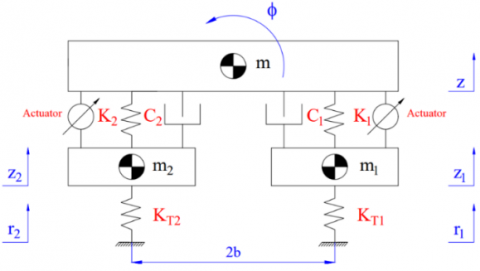
In this research, a half dynamics model is used to describe the vehicle's oscillations (Figure 1). Separating the sprung mass and the un-sprung mass, this model consists of four degrees of freedom.
Figure 1. Half dynamics model
The equations describing the vehicle's oscillation is given below:
$m\ddot{z}={{F}_{K1}}+{{F}_{C1}}-{{F}_{A1}}+{{F}_{K2}}+{{F}_{C2}}+{{F}_{A2}}$ (2)
$J\ddot{\phi }=\left( {{F}_{C1}}+{{F}_{K1}}-{{F}_{C2}}-{{F}_{K2}}-{{F}_{A1}}-{{F}_{A2}} \right)b$ (3)
${{m}_{1}}{{\ddot{z}}_{1}}={{F}_{KT1}}-{{F}_{K1}}-{{F}_{C1}}+{{F}_{A1}}$ (4)
${{m}_{2}}{{\ddot{z}}_{2}}={{F}_{KT2}}-{{F}_{K2}}-{{F}_{C2}}-{{F}_{A2}}$ (5)
where,
Force of the spring:
${{F}_{K1}}={{K}_{1}}\left( {{z}_{1}}-z-b\phi \right)$ (6)
${{F}_{K2}}={{K}_{2}}\left( {{z}_{2}}-z+b\phi \right)$ (7)
Force of the damper:
${{F}_{C1}}={{C}_{1}}\left( {{{\dot{z}}}_{1}}-\dot{z}-b\dot{\phi } \right)$ (8)
${{F}_{C2}}={{C}_{2}}\left( {{{\dot{z}}}_{2}}-\dot{z}+b\dot{\phi } \right)$ (9)
Force of the tire:
${{F}_{KT1}}={{K}_{T1}}\left( {{r}_{1}}-{{z}_{1}} \right)$ (10)
${{F}_{KT2}}={{K}_{T2}}\left( {{r}_{2}}-{{z}_{2}} \right)$ (11)
For the oscillation system to be stable, the force generated by the actuators on both sides of the suspension system needs to be of equal value. Therefore:
${{F}_{A1}}={{F}_{A2}}=u$ (12)
Substituting the values of the binding force into the equations above, and it can be rewritten as:
$\begin{align} & m\ddot{z}=-\left( {{K}_{1}}+{{K}_{2}} \right)z-\left( {{C}_{1}}+{{C}_{2}} \right)\dot{z}-\left( {{K}_{1}}-{{K}_{2}} \right)b\phi \\ & \,\,\,\,\,\,\,\,\,\,\,\,-\left( {{C}_{1}}-{{C}_{2}} \right)b\dot{\phi }+{{K}_{1}}{{z}_{1}}+{{C}_{1}}{{{\dot{z}}}_{1}}+{{K}_{2}}{{z}_{2}}+{{C}_{2}}{{{\dot{z}}}_{2}} \\ \end{align}$ (13)
$\begin{align} & J\ddot{\phi }=-\left( {{K}_{1}}-{{K}_{2}} \right)bz-\left( {{C}_{1}}-{{C}_{2}} \right)b\dot{z}-\left( {{K}_{1}}+{{K}_{2}} \right){{b}^{2}}\phi \\ & \,\,\,\,\,\,\,\,\,\,\,\,-\left( {{C}_{1}}+{{C}_{2}} \right){{b}^{2}}\dot{\phi }+{{K}_{1}}b{{z}_{1}}+{{C}_{1}}b{{{\dot{z}}}_{1}} \\ & \,\,\,\,\,\,\,\,\,\,\,-{{K}_{2}}b{{z}_{2}}-{{C}_{2}}b{{{\dot{z}}}_{2}}-2bu \\ \end{align}$ (14)
$\begin{align} & {{m}_{1}}{{{\ddot{z}}}_{1}}={{K}_{1}}z+{{C}_{1}}\dot{z}+{{K}_{1}}b\phi +{{C}_{1}}b\dot{\phi } \\ & \,\,\,\,\,\,\,\,\,\,\,\,\,\,-\left( {{K}_{1}}+{{K}_{T1}} \right){{z}_{1}}-{{C}_{1}}{{{\dot{z}}}_{1}}+u \\ \end{align}$ (15)
$\begin{align} & {{m}_{2}}{{{\ddot{z}}}_{2}}={{K}_{2}}z+{{C}_{2}}\dot{z}-{{K}_{2}}b\phi -{{C}_{2}}b\dot{\phi } \\ & \,\,\,\,\,\,\,\,\,\,\,\,\,\,-\left( {{K}_{2}}+{{K}_{T2}} \right){{z}_{2}}-{{C}_{2}}{{{\dot{z}}}_{2}}-u \\ \end{align}$ (16)
2.2 LQR controller and triple in-loops algorithm
Let:
$\begin{array}{llll}x_{1}=z . & x_{2}=\dot{x}_{1} & x_{3}=\phi & x_{4}=\dot{x}_{3} \\ x_{5}=z & x_{6}=\dot{x}_{5} & x_{7}=z_{2} & x_{8}=\dot{x}_{7}\end{array}$
The equations that have been established can be rewritten in matrix form as follows:
$\dot{x}=Ax+Bu+Cr$ (17)
where, A is the state matrix and B is the control signal matrix.
$A=\left[\begin{array}{cccccccc}0 & 1 & 0 & 0 & 0 & 0 & 0 & 0 \\ -\frac{\left(K_{1}+K_{2}\right)}{m} & -\frac{\left(C_{1}+C_{2}\right)}{m} & -\frac{\left(K_{1}-K_{2}\right) b}{m} & -\frac{\left(C_{1}-C_{2}\right) b}{m} & \frac{K_{1}}{m} & \frac{C_{1}}{m} & \frac{K_{2}}{m} & \frac{C_{2}}{m} \\ 0 & 0 & 0 & 1 & 0 & 0 & 0 & 0 \\ -\frac{\left(K_{1}-K_{2}\right) b}{J} & -\frac{\left(C_{1}-C_{2}\right) b}{J} & -\frac{\left(K_{1}+K_{2}\right) b^{2}}{J} & -\frac{\left(C_{1}+C_{2}\right) b^{2}}{J} & \frac{K_{1} b}{J} & \frac{C_{1} b}{J} & -\frac{K_{2} b}{J} & -\frac{C_{2} b}{J} \\ 0 & 0 & 0 & 0 & 0 & 1 & 0 & 0 \\ \frac{K_{1}}{m_{1}} & \frac{C_{1}}{m_{1}} & \frac{K_{1} b}{m_{1}} & \frac{C_{1} b}{m_{1}} & -\frac{\left(K_{1}+K_{T 1}\right)}{m_{1}} & -\frac{C_{1}}{m_{1}} & 0 & 0 \\ 0 & 0 & 0 & 0 & 0 & 0 & 0 & \\ \frac{K_{2}}{m_{2}} & \frac{C_{2}}{m_{2}} & -\frac{K_{2} b}{m_{2}} & -\frac{C_{2} b}{m_{2}} & 0 & 0 & -\frac{\left(K_{2}+K_{T 2}\right)}{m_{2}} & -\frac{C_{2}}{m_{2}}\end{array}\right]$
$B={{\left[ \begin{matrix} \begin{matrix} 0 & 0 & 0 & -\frac{2b}{J} \\ \end{matrix} & 0 & \frac{1}{{{m}_{1}}} & \begin{matrix} 0 & -\frac{1}{{{m}_{2}}} \\ \end{matrix} \\ \end{matrix} \right]}^{T}}$
The control signal is determined based on the state feedback controller R [54].
$u=-Rx$ (18)
For the system to be stable, the value of the cost function must be minimal [55].
$Q=\frac{1}{2}\int\limits_{0}^{\infty }{\left( {{x}^{T}}Ex+{{u}^{T}}Fu \right)dt\xrightarrow{R}min}$ (19)
where, E is the output matrix, F is the navigation matrix.
$E=\left[\begin{array}{cccccccc}\gamma_{1} \times 10^{\lambda_{1}} & 0 & 0 & 0 & 0 & 0 & 0 & 0 \\ 0 & \gamma_{2} \times 10^{\lambda_{2}} & 0 & 0 & 0 & 0 & 0 & 0 \\ 0 & 0 & \gamma_{3} \times 10^{\lambda_{3}} & 0 & 0 & 0 & 0 & 0 \\ 0 & 0 & 0 & \gamma_{4} \times 10^{\lambda_{4}} & 0 & 0 & 0 & 0 \\ 0 & 0 & 0 & 0 & \gamma_{5} \times 10^{\lambda_{5}} & 0 & 0 & 0 \\ 0 & 0 & 0 & 0 & 0 & \gamma_{6} \times 10^{\lambda_{6}} & 0 & 0 \\ 0 & 0 & 0 & 0 & 0 & 0 & \gamma_{7} \times 10^{\lambda_{7}} & 0 \\ 0 & 0 & 0 & 0 & 0 & 0 & 0 & \gamma_{8} \times 10^{\lambda_{8}}\end{array}\right] F=\left[ \delta \right] $
According to Lyapunov's theory, the matrix R can be defined as follows:
$R={{F}^{-1}}{{B}^{T}}P$ (20)
where, P is the solution of the Riccati algebraic equation:
$PB{{F}^{-1}}{{B}^{T}}P-PA-{{A}^{T}}P=E$ (21)
Figure 2. Optimal algorithm diagram
Based on the presented formulas, if the coefficients of matrix E and matrix F can be selected appropriately, the LQR controller will achieve the highest efficiency. Therefore, optimization of controller parameters needs to be performed.
The optimal algorithm diagram is shown in Figure 2. According to this diagram, three parameters are optimized, including gi, li, and d. The process of optimizing parameters is carried out in three stages. At the first stage, the limits of the parameters will be determined. This limit is determined based on the stability conditions of the system. The results of the first stage will help the optimization process go faster. In the second stage, the simulation is performed corresponding to the parameters, which change continuously closed in-loops. The results of the second stage are the average and maximum values of the roll angle of the sprung mass and the angular acceleration of the sprung mass. The results obtained from the second stage will be compared with each other. In the final stage, the parameters will be selected, so that, the oscillation of the vehicle is minimal. After the controller parameters have been optimized, the simulation will be performed again to verify the obtained results.
2.3 Simulation conditions
The simulation takes place when the controller parameters have been determined. In this paper, the vehicle's oscillations will be compared in three cases:
In the first case, the vehicle uses a conventional passive suspension system.
In the second case, the vehicle uses an active suspension system, and the controller's optimization is done through double in-loops (determining li and d).
In the third case, the vehicle uses an active suspension system, the controller's optimization is done through triple in-loops (determining gi, li, and d).
The vehicle specifications are shown in Table 2.
Table 2. Specification of the vehicle
|
Symbol |
Description |
Value |
Unit |
|
m |
Sprung mass |
900 |
kg |
|
mi |
Un-sprung mass |
65 |
kg |
|
Ki |
Stiffness of spring |
40000 |
Nm-1 |
|
Ci |
Damping coefficient |
3500 |
Nsm-1 |
|
KTi |
Stiffness of tire |
170000 |
Nm-1 |
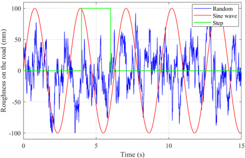
Figure 3. Roughness on the road
The excitement from the road surface is the direct cause of the vehicle's oscillations. In this research, three types of stimulation were used corresponding to the three survey situations (Figure 3), including:
The first situation: Sine wave stimulation:
$r\left( t \right)=Rsin\left( 2\pi ft+\varphi \right)$ (22)
The second situation: Random stimulation:
$r\left( t \right)=\int\limits_{0}^{\tau }{\left[ 2\pi \sqrt{Gv\omega \left( \tau \right)}-2\pi fr\left( \tau \right) \right]}d\tau $ (23)
The third situation: Step stimulation:
$r\left( t \right)=\left\{ \begin{align} & 0,t<{{t}_{0}} \\ & h,{{t}_{0}}\le t\le {{t}_{i}} \\ & 0,t>{{t}_{i}} \\ \end{align} \right.$ (24)
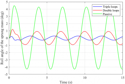
3.1 Sine wave
Sine wave excitation is commonly used in control problems. This excitation has a cyclic form with a low frequency. With this type of excitation, the periodic oscillation is repeated according to a certain law.
Figure 4. Roll angle of the sprung mass
Figure 5. Angular acceleration of the sprung mass
Figure 4 shows the change in the roll angle of the sprung mass over time. In the case of the vehicle using a passive suspension system, the roll angle of the vehicle body is large. Its maximum value can reach 4.47°. If this system is replaced by an active suspension system, the maximum value of the roll angle can be significantly reduced. This value reaches 1.21° and 0.30° respectively for the double in-loops control algorithm and the triple in-loops control algorithm. Besides, the average value of the roll angle, which is calculated according to (1), is also shown. In this way, its average value is 3.03°, 0.66°, and 0.20° respectively for the three simulation situations.
The angular acceleration of the sprung mass is a characteristic of the vehicle's oscillations. If this value is large, the vehicle's stability cannot be guaranteed. The value of the angular acceleration of the sprung mass is shown in Figure 5. The maximum value of the acceleration is 1.03 (rad/s2), 0.67 (rad/s2) and 0.32 (rad/s2), respectively for the above three cases. Also, their average values in terms of RMS are 0.25 (rad/s2), 0.09 (rad/s2), and 0.04 (rad/s2). Obviously, the difference between using passive suspension and active suspension is huge.
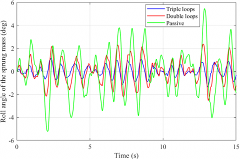
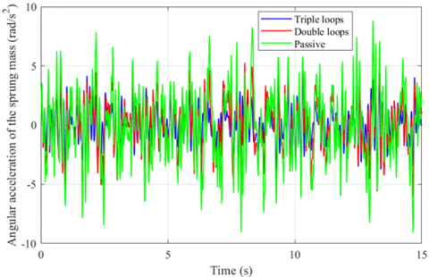
3.2 Random
Random excitation usually occurs when the vehicle is moving on the actual road. With this excitation, the amplitude and frequency of the oscillation change continuously. As a result, the vehicle may experience strong oscillations.
Figure 6. Roll angle of the sprung mass
In Figure 6, the variation of the roll angle of the vehicle body is shown. Accordingly, the maximum roll angle can be up to 5.47°, 2.54°, and 1.37°, respectively, for the cases introduced in the paper. Besides, the average value of oscillation is also larger than the case of using cyclic excitation. These values are 1.97°, 1.06°, and 0.49°, respectively. According to this result, if the vehicle uses a conventional passive suspension, the value of the roll angle can be 4.02 times that of using an active suspension system controlled by a triple in-loops algorithm.
Figure 7. Angular acceleration of the sprung mass
In this case, the angular acceleration of the sprung mass can be very large (Figure 7). At some point, the angular acceleration was as high as 9.10 (rad/s2). However, this value can be reduced to only 7.95 (rad/s2) and 4.71 (rad/s2) when the mechanical suspension system is replaced by the active suspension system. In addition, the average value of the angular acceleration that is calculated according to the RMS also has a very large difference, and they can be 1.93 times each other.
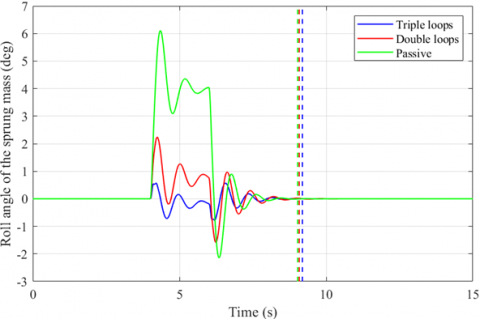
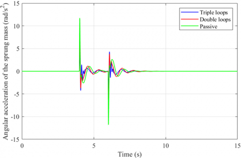
3.3 Step
Step excitation is also commonly used in oscillation problems. Its frequency is low. However, the change of the stimulus signal is abrupt. So, it can cause big oscillation for the vehicle. In this paper, step excitation with a single pulse is proposed. At time t = 4 (s), the vehicle starts to oscillate (Figure 8). The roll angle of the sprung mass increases gradually to the maximum value. If a passive suspension is fitted on the vehicle, this value can go up to 6.11°. At the same time, it will cause the vehicle's acceleration to increase rapidly, reaching 11.81 (rad/s2). The LQR controller with a triple in-loops algorithm can effectively reduce these values. When this controller is used, the value of the oscillation is only 0.78° and 4.32 (rad/s2) (Figure 9).
Some control methods can lead to continuous oscillations after the excitation ceases to exist. This can greatly affect the smoothness of the vehicle. With the designed triple in-loops algorithm, the end time of the control process will be equivalent to the end time of the passive suspension system. At time t = 9.03 (s), 9.19 (s), and 9.08 (s), the roll angle's value is approximately 0.001°, the control process can be considered stable.
The results of the simulation are shown in Table 3 and Table 4. In which the maximum and average values of the roll angle of the sprung mass and the angular acceleration of the sprung mass are calculated exactly. This data corresponds to three simulation cases and three survey conditions.
Figure 8. Roll angle of the sprung mass
Figure 9. Angular acceleration of the sprung mass
Table 3. Average value
|
|
Roll angle |
Acceleration |
Roll angle |
Acceleration |
Roll angle |
Acceleration |
|
Random |
0.49 |
1.55 |
1.06 |
2.30 |
1.97 |
2.99 |
|
Sine wave |
0.20 |
0.04 |
0.66 |
0.09 |
3.03 |
0.25 |
|
Step |
0.17 |
0.45 |
0.43 |
0.73 |
1.55 |
0.98 |
Table 4. Maximum value
|
|
Roll angle |
Acceleration |
Roll angle |
Acceleration |
Roll angle |
Acceleration |
|
Random |
1.37 |
4.71 |
2.54 |
7.95 |
5.47 |
9.10 |
|
Sine wave |
0.30 |
0.32 |
1.21 |
0.67 |
4.47 |
1.03 |
|
Step |
0.78 |
4.32 |
2.24 |
8.35 |
6.11 |
11.81 |
The excitement from the road surface is what causes the vehicle to oscillate. The suspension system plays an important role in maintaining and ensuring the stability of the vehicle against this stimulation. In many cases, conventional mechanical suspensions are not able to meet the vehicle's comfort requirements. Therefore, the active suspension is used to replace the passive suspension. The performance of the active suspension system depends on its controller. In this paper, the LQR controller is used.
This paper has established a half dynamics model of the vehicle to describe its oscillations. Besides, the triple in-loops optimization algorithm is also introduced. The controller parameters can be optimally calculated based on the proposed algorithm. This method brings high efficiency to the calculation process. In addition, the execution time is also very short. Simultaneously, the simulation is conducted for three survey cases and three stimulus situations from the road surface. The results of the research have shown the outstanding performance of the optimization algorithm, which has been shown in the paper. When the vehicle uses the active suspension system, the maximum and average values of oscillations are greatly reduced compared to using the passive suspension system. Besides, the triple in-loops optimization algorithm provides more stability and convenience than the double in-loops algorithm. The performance of the controller is very high, and it works stably in many situations. These are the positive results brought about by the new algorithm, which is mentioned in the paper.
This research only conducts calculations and simulations. There are many influencing factors that have been overlooked. Therefore, it is necessary to have an experimental process to verify the results of the paper. This is the basis to be able to conduct experiments based on this control method. In the future, intelligent control algorithms can be used to better optimize the parameters of the LQR controller.
|
FA |
Actuator force, N |
|
FC |
Damper force, N |
|
FK |
Spring force, N |
|
FKT |
Tire force, N |
|
J |
Moment of inertia, kgm2 |
|
m |
Sprung mass, kg |
|
mi |
Un-sprung mass, kg |
|
ri |
Roughness on the road, m |
|
z |
Displacement of the sprung mass, m |
|
zi |
Displacement of the un-sprung mass, m |
|
Greek symbols |
|
|
$\phi$ |
Roll angle, rad |
[1] Wibowo, Lambang, L., Muhayat, N. (2017). Simulation and analysis of vertical displacement characteristics of three wheels reverse trike vehicle with PID controller application. In AIP Conference Proceedings, 1867(1): 020021. https://doi.org/10.1063/1.4994424
[2] Nguyen, T.A. (2021). Advance the stability of the vehicle by using the pneumatic suspension system integrated with the hydraulic actuator. Latin American Journal of Solids and Structures, 18(7): e403. https://doi.org/10.1590/1679-78256621
[3] Melo, F.J.M.Q., Pereira, A.B.P., Morais, A.B. (2018). The simulation of an automotive air spring suspension using a pseudo-dynamic procedure. Applied Sciences, 8(7): 1049. https://doi.org/10.3390/app8071049
[4] Ren, H., Zhao, Y., Chen, S., Liu, G. (2015). State observer based adaptive sliding mode control for semi-active suspension systems. Journal of Vibroengineering, 17(3): 1464-1475. https://doi.org/10.1080/00423114.2015.1122818
[5] Basargan, H., Mihály, A., Gáspár, P., Sename, O. (2020). Adaptive semi-active suspension and cruise control through LPV technique. Applied Sciences, 11(1): 290. https://doi.org/10.3390/app11010290
[6] Aljarbouh, A., Fayza, M. (2020). Hybrid modelling and sliding mode control of semi-active suspension systems for both ride comfort and roadholding. Symmetry, 12(8): 1286. https://doi.org/10.3390/sym12081286
[7] Maurya, V.K., Bhangal, N.S. (2018). Optimal control of vehicle active suspension system. Journal of Automation and Control Engineering, 6(1): 22-26. http://doi.org/10.18178/joace.6.1.22-26
[8] Avesh, M., Srivastava, R. (2012). Modelling simulation and control of active suspension system in MATLAB simulink environment. Proceedings of the 2012 Students Conference on Engineering and Systems, Allahabad, India, pp. 1-6. https://doi.org/10.1109/SCES.2012.6199124
[9] Nguyen, M.L., Tran, T.T.H., Nguyen, T.A., Nguyen, D.N., Dang, N.D. (2022). Application of MIMO control algorithm for active suspension system: A new model with 5 state variables. Latin American Journal of Solids and Structures, 19: e435. https://doi.org/10.1590/1679-78256992
[10] Bello, M.M., Shafie, A.A., Khan, R. (2015). Active vehicle suspension control using full state-feedback controller. Advanced Materials Research, 1115: 440-445. http://dx.doi.org/10.4028/www.scientific.net/AMR.1115.440
[11] Shafie, A.A., Bello, M.M., Khan, R.M. (2015). Active vehicle suspension control using electrohydraulic actuator on rough road terrain. Journal of Advanced Research in Applied Mechanics, 9(1): 15-30.
[12] Talib, M.H.A., Darus, I.Z.M. (2013). Self-tuning PID controller for active suspension system with hydraulic actuator. Proceedings of the 2013 IEEE Symposium on Computers & Informatics, Langkawi, Malaysia, pp. 86-91. https://doi.org/10.1109/ISCI.2013.6612381
[13] Nguyen, T.A. (2021). Improving the comfort of the vehicle based on using the active suspension system controlled by the double-integrated controller. Shock and Vibration, 2021: 1426003. https://doi.org/10.1155/2021/1426003
[14] Munawwarah, S., Yakub, F. (2021). Control analysis of vehicle ride comfort through integrated control devices on the quarter and half car active suspension systems. Proceedings of the Institution of Mechanical Engineers, Part D: Journal of Automobile Engineering, 235(5): 1256-1268. https://doi.org/10.1177%2F0954407020968300
[15] Heidari, M., Homaei, H. (2013). Design a PID controller for suspension system by back propagation neural network. Journal of Engineering, 2013: 421543. https://doi.org/10.1155/2013/421543
[16] Talib, M.H.A. (2020). Vibration control of semi-active suspension system using PID controller with advanced firely algorithm and particle swarm optimization. Journal of Ambient Intelligence and Humanized Computing, 12: 1119-1137. https://doi.org/10.1007/s12652-020-02158-w
[17] Nagarkar, M.P., Bhalerao, Y.J., Patil, G.V., Patil, R.Z. (2018). Multi-objective optimization of nonlinear quarter car suspension system–PID and LQR control. Procedia Manufacturing, 20: 420-427. https://doi.org/10.1016/j.promfg.2018.02.061
[18] Nagarkar, M.P., Vikhe, G.J., Borole, K.R., Nandedkar, V.M. (2011). Active control of quarter-car suspension system using linear quadratic regulator. International Journal of Automotive and Mechanical Engineering, 3(1): 364-372. http://dx.doi.org/10.15282/ijame.3.2011.11.0030
[19] Soliman, A.M.A. (2011). Adaptive LQR control strategy for active suspension system. SAE Technical Paper, 2011-01-0430. https://doi.org/10.4271/2011-01-0430
[20] Putra, S.M.S.M., Yakub, F., Rasid, Z.A., Zaki, S.A., Ali, M.S.M., Daud, Z.H.C. (2018). Linear quadratic regulator based control device for active suspension system with enhanced vehicle ride comfort. Journal of the Society of Automotive Engineers Malaysia, 2(3): 289-305.
[21] Anh, N.T. (2020). Control an active suspension system by using PID and LQR controller. International Journal of Mechanical and Production Engineering Research and Development, 10(3): 7003-7012. http://dx.doi.org/10.24247/ijmperdjun2020662
[22] Chai, L., Sun, T. (2010). The design of LQG controller for active suspension based on analytic hierarchy process. Mathematical Problems in Engineering, 2010: 701915. https://doi.org/10.1155/2010/701951
[23] Xia, R.X., Li, J.H., He, J., Shi, D.F., Zhang, Y. (2015). Linear-quadratic-Gaussian controller for truck active suspension based on cargo integrity. Advances in Mechanical Engineering, 7(12): 1687814015620320. https://doi.org/10.1177%2F1687814015620320
[24] Pang, H., Chen, Y., Chen, J., Liu, X. (2017). Design of LQG controller for active suspension without considering road input signals. Shock and Vibration, 2017: 6573567. https://doi.org/10.1155/2017/6573567
[25] Chen, S.A., Cai, Y.M., Wang, J., Yao, M. (2018). A novel LQG controller of active suspension system for vehicle roll safety. International Journal of Control, Automation and Systems, 16(5): 2203-2213. http://dx.doi.org/10.1007/s12555-017-0159-2
[26] Babawuro, A.Y., Tahir, N.M., Muhammed, M., Sambo, A.U. (2020). Optimized state feedback control of quarter car active suspension system based on LMI algorithm. In Journal of Physics: Conference Series, 1502: 012019. http://dx.doi.org/10.1088/1742-6596/1502/1/012019
[27] Bai, R., Guo, D. (2018). Sliding-mode control of the active suspension system with the dynamics of a hydraulic actuator. Complexity, 2018: 5907208. https://doi.org/10.1155/2018/5907208
[28] Nguyen, T.A. (2021). Study on the sliding mode control method for the active suspension system. International Journal of Applied Science and Engineering, 18(5): 2021069. https://doi.org/10.6703/IJASE.202109_18(5).006
[29] Deshpande, V.S., Bhaskara, M., Phadke, S.B. (2012). Sliding mode control of active suspension systems using a disturbance observer. Proceedings of the 12th International Workshop on Variable Structure Systems, Mumbai, India. https://doi.org/10.1109/VSS.2012.6163480
[30] Lin, B., Su, X., Li, X. (2018). Fuzzy sliding mode control for active suspension system with proportional differential sliding mode observer. Asian Journal of Control, 21(1): 1-13. https://doi.org/10.1002/asjc.1882
[31] Alves, U.N.L., Garcia, J.P.F., Teixeira, M., Garcia, S.C., Rodrigues, F.B. (2014). Sliding mode control for active suspension system with data acquisition delay. Mathematical Problems in Engineering, 2014: 529293. https://doi.org/10.1155/2014/529293
[32] Sun, W., Zhao, Z., Gao, H. (2013). Saturated adaptive robust control for active suspension systems. IEEE Transactions on Industrial Electronics, 60(9): 3889-3896. https://doi.org/10.1109/TIE.2012.2206340
[33] Yamada, F., Suzuki, K., Toda, T., Chen, G., Takami, I. (2016). Robust control of active suspension to improve ride comfort with structural constraints. In 2016 IEEE 14th International Workshop on Advanced Motion Control (AMC), pp. 103-108. https://doi.org/10.1109/AMC.2016.7496335
[34] Singh, N., Chhabra, H., Bhangal, K. (2016). Robust control of vehicle active suspension system. International Journal of Control and Automation, 9(4): 149-160. http://dx.doi.org/10.14257/ijca.2016.9.4.15
[35] Burkan, R., Ozguney, O.C., Ozbek, C. (2017). Model reaching adaptive-robust control law for vibration isolation systems with parametric uncertainty. Journal of Vibroengineering, 20(1): 300-309. https://doi.org/10.21595/jve.2017.18429
[36] Gudarzi, M., Oveisi, A. (2014). Robust control for ride comfort improvement of an active suspension system considering uncertain driver’s biodynamics. Journal of Low Frequency Noise, Vibration and Active Control, 33(3): 317-340. https://doi.org/10.1260%2F0263-0923.33.3.317
[37] Huang, Y., Na, J., Wu, X., Gao, G.B., Guo, Y. (2018). Robust adaptive control for vehicle active suspension systems with uncertain dynamics. Transactions of the Institute of Measurement and Control, 40(4): 1237-1249. https://doi.org/10.1177%2F0142331216678312
[38] Fu, Z.J., Dong, X.Y. (2021). H optimal control of vehicle active suspension systems in two times scales. Automatika, 62(2): 284-292. http://dx.doi.org/10.1080/00051144.2021.1935610
[39] Rizvi, S.M.H., Abid, M., Khan, A.Q., Satti, S.G., Latif, J. (2018). H∞ control of 8 degrees of freedom vehicle active suspension system. Journal of King Saud University-Engineering Sciences, 30(2): 161-169. https://doi.org/10.1016/j.jksues.2016.02.004
[40] Wu, H., Zheng, L., Li, Y., Zhang, Z., Yu, Y. (2020). Robust control for active suspension of hub-driven electric vehicles subject to in-wheel motor magnetic force oscillation. Applied Sciences, 10(11): 3929. https://doi.org/10.3390/app10113929
[41] Li, W., Du, H., Ning, D., Li, W. (2019). Robust adaptive sliding mode PI control for active vehicle seat suspension systems. In 2019 Chinese Control and Decision Conference (CCDC), pp. 5403-5408. https://doi.org/10.1109/CCDC.2019.8832368
[42] Kaleemullah, M., Faris, W.F., Ghazaly, N.M. (2019). Analysis of active suspension control policies for vehicle using robust controllers. International Journal of Advanced Science and Technology, 28(16): 836-855.
[43] Fazeli, S., Motlagh, M.R.J., Moarefianpur, A. (2021). An adaptive approach for vehicle suspension system control in presence of uncertainty and unknow actuator time delay. Systems Science & Control Engineering, 9(1): 117-126. https://doi.org/10.1080/21642583.2020.1850369
[44] Huang, Y., Na, J., Wu, X., Liu, X., Guo, Y. (2015). Adaptive control of nonlinear uncertain active suspension systems with prescribed performance. ISA Transactions, 54: 145-155. https://doi.org/10.1016/j.isatra.2014.05.025
[45] Fu, Z.J., Li, B., Ning, X.B., Xie, W.D. (2017). Online adaptive optimal control of vehicle active suspension systems using single-network approximate dynamic programming. Mathematical Problems in Engineering, 2017. https://doi.org/10.1155/2017/4575926
[46] Palanisamy, S., Karuppan, S. (2016). Fuzzy control of active suspension system. Journal of Vibroengineering, 18(5): 3197-3204. https://doi.org/10.21595/jve.2016.16699
[47] Na, J., Huang, Y., Wu, X., Su, S.F., Li, G. (2019). Adaptive finite-time fuzzy control of nonlinear active suspension systems with input delay. IEEE Transactions on Cybernetics, 50(6): 2639-2650. https://doi.org/10.1109/TCYB.2019.2894724
[48] Nan, Y., Shi, W., Fang, P. (2016). Improvement of ride performance with an active suspension based on fuzzy logic control. Journal of Vibroengineering, 18(6): 3941-3955. https://doi.org/10.21595/jve.2016.16827
[49] Haddar, M., Chaari, R., Baslamisli, S.C., Chaari, F., Haddar, M. (2021). Intelligent optimal controller design applied to quarter car model based on non-asymptotic observer for improved vehicle dynamics. Proceedings of the Institution of Mechanical Engineers, Part I: Journal of Systems and Control Engineering, 235(6): 929-942. https://doi.org/10.1177%2F0959651820958831
[50] Haddar, M., Chaari, R., Baslamisli, S.C., Chaari, F., Haddar, M. (2019). Intelligent PD controller design for active suspension system based on robust model-free control strategy. Proceedings of the Institution of Mechanical Engineers, Part C: Journal of Mechanical Engineering Science, 233(14): 4863-4880. https://doi.org/ 10.1177/0954406219836443
[51] Zhao, F., Dong, M., Qin, Y., Gu, L., Guan, J. (2015). Adaptive neural-sliding mode control of active suspension system for camera stabilization. Shock and Vibration, 2015: 542364. https://doi.org/10.1155/2015/542364
[52] Nguyen, T.A. (2022). A novel sliding mode control algorithm for an active suspension system considering with the hydraulic actuator. Latin American Journal of Solids and Structures, 19(1): e424. https://doi.org/10.1590/1679-78256883
[53] Nguyen, T.A. (2021). Advance the efficiency of an active suspension system by the sliding mode control algorithm with five state variables. IEEE Access, 9: 164368-164378. https://doi.org/10.1109/ACCESS.2021.3134990
[54] Valencia-Rivera, G.H., Merchan-Villalba, L.R., Tapia-Tinoco, G., Lozano-Garcia, J.M., Ibarra-Manzano, M.A., Avina-Cervantes, J.G. (2020). Hybrid LQR-PI control for microgrids under unbalanced linear and nonlinear loads. Mathematics, 8(7): 1096. https://doi.org/10.3390/math8071096
[55] Hajiyev, C., Vural, S.Y. (2013). LQR controller with Kalman estimator applied to UAV longitudinal dynamics. Positioning, 4: 36-41. http://dx.doi.org/10.4236/pos.2013.41005